8 Specific examples

In this section I will illustrate a series of examples of specific more complex scenarios. They can be all run independently and used as a basis for your own specific scenarios.

Here is a table summarising which functionalities are used in which example:

Functionality showcase	Example
bd.params	reducing speciation rate, generating a subtree with no extinction
make.events	mass extinction, negative trait extinction, background extinction, reducing speciation rate, changing trait process, changing trait correlation, changing modifiers, change branch length, generating a subtree with no extinction, generating a subtree with a different process
make.traits	negative trait extinction, changing trait process, changing trait correlation, generating a subtree with a different process
make.modifiers	changing modifiers, change branch length

And more specifically for the events:

Functionality showcase	Example
age.condition	mass extinction, negative trait extinction, reducing speciation rate, changing trait process, changing modifiers
random.extinction	mass extinction
trait.extinction	negative trait extinction
taxa.condition	background extinction, change branch length
bd.params.update	background extinction, reducing speciation rate
traits.update	changing trait process, changing trait correlation
trait.condition	changing trait correlation, generating a subtree with a different process
modifiers.update	changing modifiers, change branch length
parent.traits	changing modifiers
founding.event	generating a subtree with no extinction, generating a subtree with a different process

8.1 Random mass extinction after some time

For this scenario, we want to generate a pure birth tree (no traits and no extinction) where 80% of the species go extinct two thirds of the way into the scenario.

For that we first need to first set our simulation parameters: we will be running the simulation for 6 time units and with a speciation rate of 1 (and extinction of 0 - default).

## Setting the parameters
stop_time_6 <- list(max.time = 6)
speciation_1 <- make.bd.params(speciation = 1)

We will then create a event that triggers when reaching half of the simulation time (using age.condition(2.5)). This event will target "taxa", i.e. the number of species, and randomly remove 80% of them (using random.extinction(0.8)):

## 80% mass extinction at time 4
mass.extinction <- make.events(
                    condition = age.condition(4),
                    target = "taxa",
                    modification = random.extinction(0.8))

Once these parameters are defined, we can run the simulations and plot the results:

## Running the simulations
set.seed(1)
results <- treats(stop.rule = stop_time_6,
                bd.params = speciation_1,
                events    = mass.extinction)
## Plotting the results
plot(results, show.tip.label = FALSE)
axisPhylo()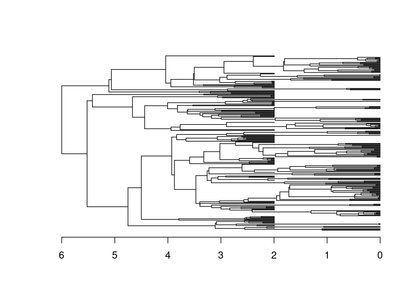

8.2 Species with negative trait values go extinct after a certain time

For this scenario, we want to generate a pure birth tree with a one dimensional Brownian Motion trait for 5 time units. We then want species with a negative trait value go extinct after 4 time units.

First we need to set up the simulation parameters: * The stopping rule (5 time units) * The birth-death parameters (speciation rate of 1)

## Simulation parameters
stop_time_5 <- list(max.time = 5)
speciation_1 <- make.bd.params(speciation = 1)

Then set up our trait which is a one dimensional Brownian Motion

## Trait
simple_bm_trait <- make.traits(n = 1, process = BM.process)

And our extinction event which triggers after reaching time 4 (age.condition(4)), targets the "taxa" and modifies the extinction for species with traits lower than 0.

## Extinction of any tips with trait < 1 at time 4
trait.extinction <- make.events(
                      target = "taxa",
                      condition = age.condition(4),
                      modification = trait.extinction(x = 0,
                                                      condition = `<`))

Once these parameters are defined, we can run the simulations and plot the results:

## Running the simulations
set.seed(7)
results <- treats(stop.rule = stop_time_5,
                bd.params = speciation_1,
                traits    = simple_bm_trait,
                events    = trait.extinction)
## Plotting the results
plot(results)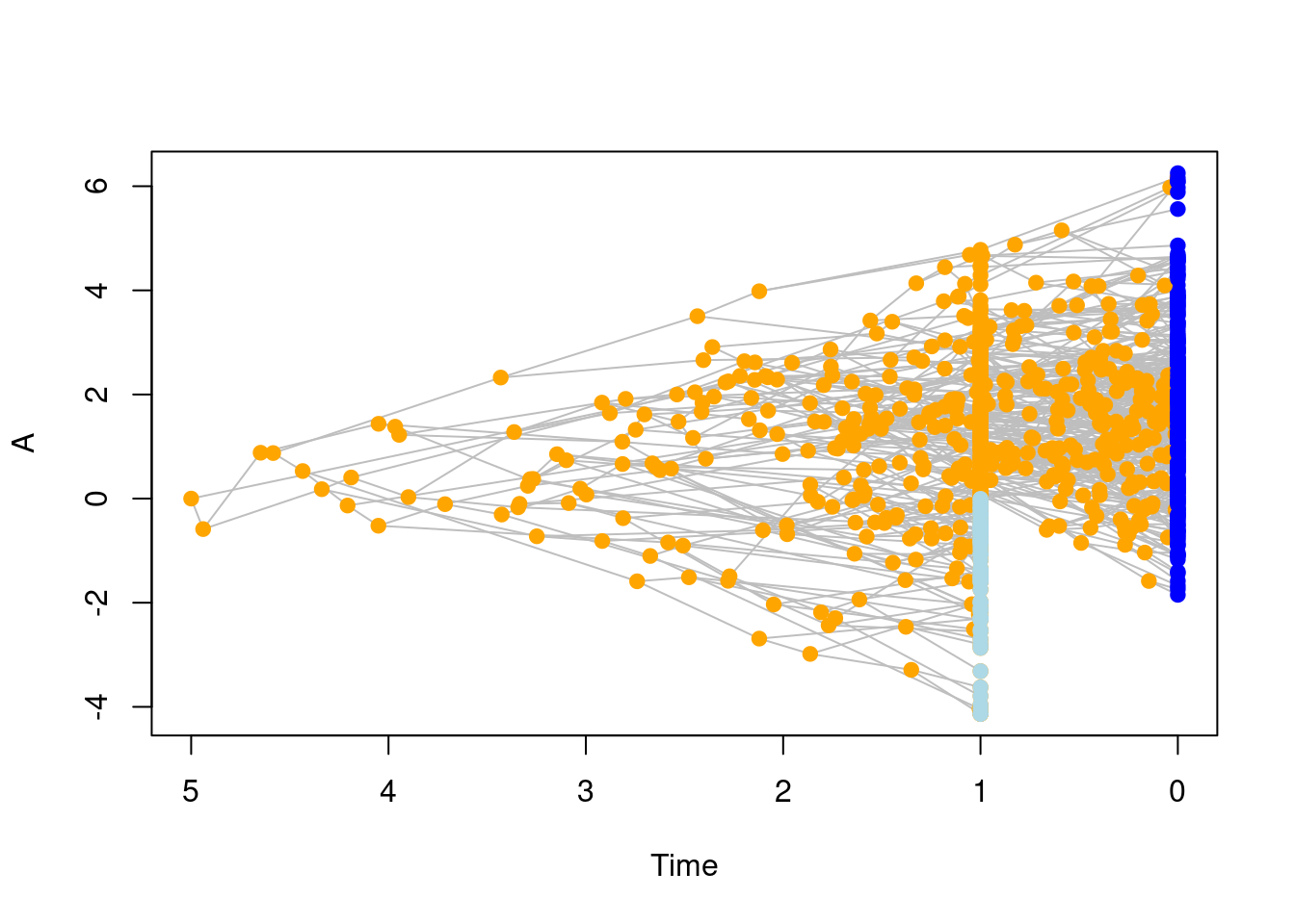

8.3 Adding a background extinction after reaching a number of living taxa

For this scenario, we want to generate a pure birth tree until reaching 50 living taxa but with an extinction rate appearing after reaching 30 taxa.

First we need to set up the simulation parameters: * The stopping rule (50 taxa max) * The birth-death parameters (speciation rate of 1)

## Simulation parameters
stop_taxa_50 <- list(max.living = 50)
speciation_1 <- make.bd.params(speciation = 1)

And our change in extinction rate event which triggers after reaching 30 taxa (taxa.condition(30)), targets the "bd.params" (birth-death parameters) sets the extinction rate to 0.5 (bd.params.update(extinction = 0.5)):

## Adding an extinction parameter after 30 taxa
background.extinction <- make.events(
                      condition = taxa.condition(30),
                      target = "bd.params",
                      modification = bd.params.update(extinction = 0.5))

Once these parameters are defined, we can run the simulations and plot the results:

## Running the simulations
set.seed(2)
results <- treats(stop.rule = stop_taxa_50,
                bd.params = speciation_1,
                events = background.extinction)
## Plotting the results
plot(results, show.tip.label = FALSE)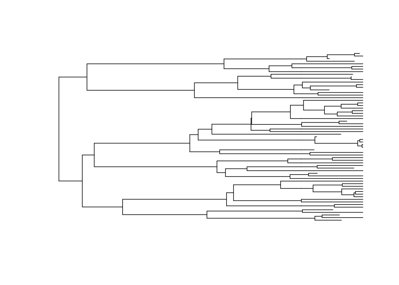

8.4 Reducing speciation rate after a certain time

For this scenario, we want to generate a birth tree for 6 times units with random speciation rates (i.e. drawn from a uniform (0.5;1) distribution) which reduces after time 4 through the simulations to a fixed value of 1/3.

First we need to set up the simulation parameters: * The stopping rule (6 time units) * The birth-death parameters (speciation randomly drawn between 0.5 and 1)

## Simulation parameters
stop_time_6 <- list(max.time = 6)
random_speciation <- make.bd.params(speciation = runif, 
                                    speciation.args = list(min = 0.5, max = 1))

And our extinction event which triggers after reaching time 4 (age.condition(4)), targets the "bd.params" and modifies the speciation rate to 1/3:

## Reducing speciation after reaching time 4
reduced.speciation <- make.events(
                      condition = age.condition(4),
                      target = "bd.params",
                      modification = bd.params.update(speciation = 1/3))

Once these parameters are defined, we can run the simulations and plot the results. We can contrast the results with the scenario without an event (but same random seed):

## No event
set.seed(42)
no_event <- treats(stop.rule = stop_time_6,
                 bd.params = random_speciation)

## Reduced speciation event
set.seed(42)
reduced_speciation_event <- treats(stop.rule = stop_time_6,
                                 bd.params = random_speciation,
                                 events = reduced.speciation)

## Plot both trees
par(mfrow = c(1, 2))
plot(no_event, main = "No event", show.tip.label = FALSE)
axisPhylo()
plot(reduced_speciation_event, 
     main = "Reduced speciation after time 5", 
     show.tip.label = FALSE)
axisPhylo()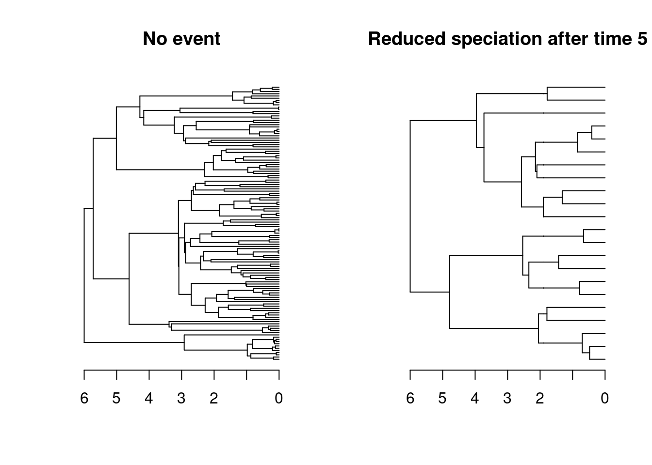

8.5 Changing the trait process after some time

For this scenario, we want to generate a pure birth tree with a one dimensional Brownian Motion trait for 5 time units which then changes to an OU process.

First we need to set up the simulation parameters: * The stopping rule (6 time units) * The birth-death parameters (speciation rate of 1)

## Simulation parameters
stop_time_6 <- list(max.time = 6)
speciation_1 <- make.bd.params(speciation = 1)

Then set up our trait which is a one dimensional Brownian Motion

## Trait
simple_bm_trait <- make.traits(n = 1, process = BM.process)

And our event which triggers after reaching time 5 (age.condition(5)), targets the "traits" and modifies the process to OU.process.

## Create an event to change the trait process
change.process.to.OU <- make.events(
                  condition    = age.condition(5),
                  target       = "traits",
                  modification = traits.update(process = OU.process))

Once these parameters are defined, we can run the simulations and plot the results. We can contrast the results with the scenario without an event (but same random seed):

## Run the simulations without change
set.seed(1)
no_change <- treats(stop.rule = stop_time_6,
                  bd.params = speciation_1,
                  traits    = simple_bm_trait)
## Run the simulations with change
set.seed(1)
process_change <- treats(stop.rule = stop_time_6,
                       bd.params = speciation_1,
                       traits    = simple_bm_trait,
                       events    = change.process.to.OU)
## Plot the results
par(mfrow = c(1,2))
plot(no_change, ylim = c(-7, 7))
plot(process_change, ylim = c(-7, 7))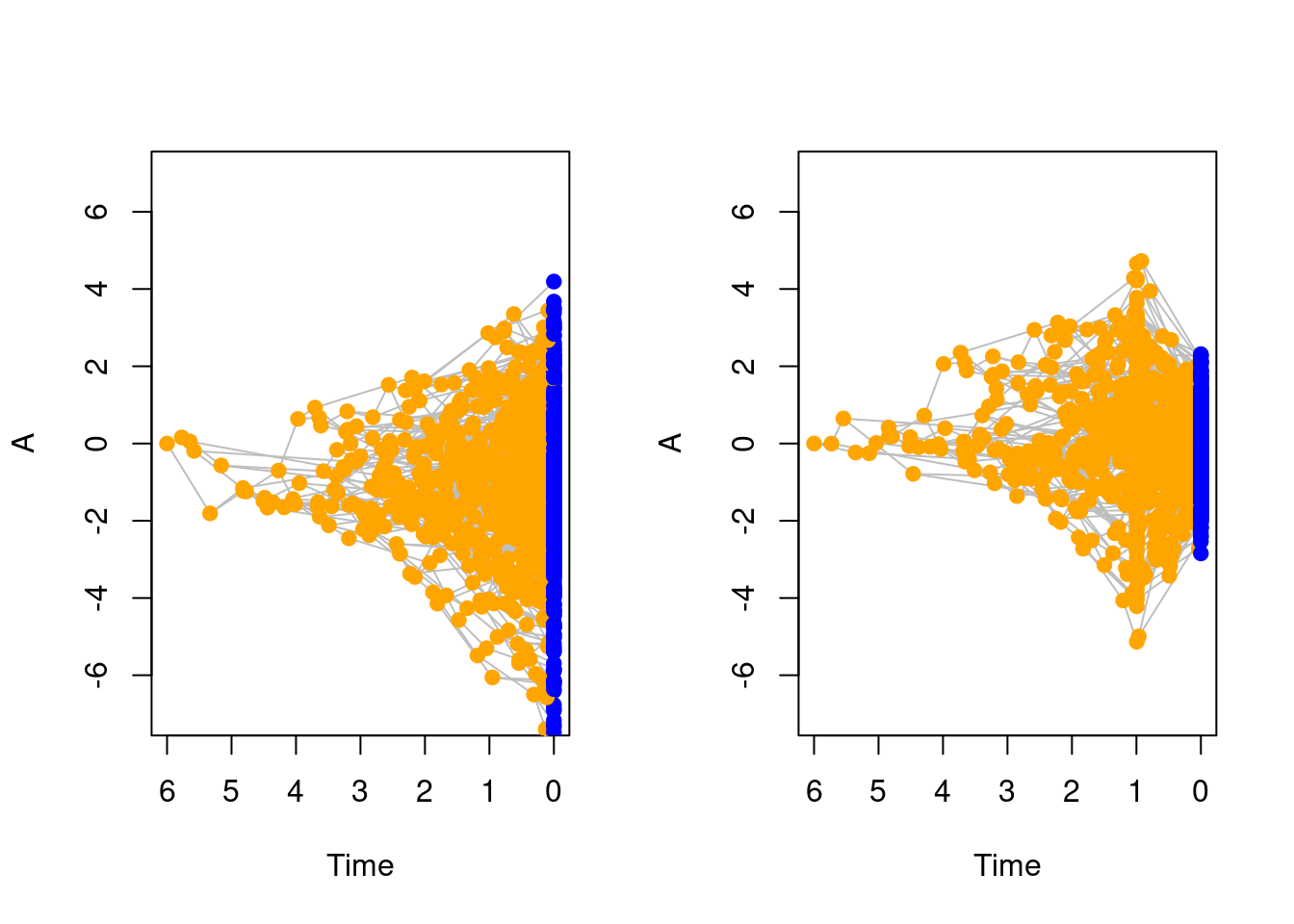

8.6 Changing trait correlation after reaching a trait value

For this scenario, we want to generate a pure birth tree with a 2 dimensional Brownian Motion trait with a strict correlation between the two dimensions (1:1) that loosen up when a taxa reaches an absolute value of 2.

First we need to set up the simulation parameters: * The stopping rule (100 taxa) * The birth-death parameters (speciation rate of 1)

## Set the parameters
stop_taxa_100 <- list(max.taxa = 100)
speciation_1 <- make.bd.params(speciation = 1)

Then set up our trait which is a 2 dimensional Brownian Motion with a correlation matrix Sigma ()

## A 2D variance covariance matrix
cor_matrix <- matrix(1, 2, 2)

## A correlated 2D Brownian Motion
correlated_2D_BM <- make.traits(n = 2, process = BM.process,
                      process.args = list(Sigma = cor_matrix))

And our event which triggers after a taxa gets the trait value 3 (trait.condition(3, absolute = TRUE)), targets the "traits" and modifies the traits correlation

## New correlation
new_cor <- matrix(c(10,3,3,2),2,2)

## Event changing a trait correlation
correlation.change <- make.events(
    condition    = trait.condition(3, absolute = TRUE),
    target       = "traits",
    modification = traits.update(process.args = list(Sigma = new_cor)))

Once these parameters are defined, we can run the simulations and plot the results. We can contrast the results with the scenario without an event (but same random seed):

## Run the simulations
set.seed(2)
no_event <- treats(stop.rule = stop_taxa_100,
                 bd.params = speciation_1,
                 traits    = correlated_2D_BM)
set.seed(2)
change_correlation <- treats(stop.rule = stop_taxa_100,
                           bd.params = speciation_1,
                           traits    = correlated_2D_BM,
                           events    = correlation.change)

## Visual testing
par(mfrow = c(1,2))
plot(no_event, trait = c(1,2), main = "Strict correlation")
plot(change_correlation, trait = c(1,2), main = "Loosened correlation")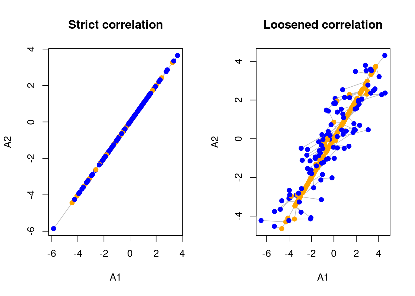

And we can visualise this change through time:

## 3D plot
plot(change_correlation, trait = c(1:2), use.3D = TRUE)
rglwidget()

8.7 Event for changing a modifier: extinction event increase for species with negative values

For this scenario, we want to generate a pure birth tree with a one dimensional Brownian Motion trait for 4 time units. After 3 time units, we want the speciation rule to increase for species which ancestors have a negative trait value.

First we need to set up the simulation parameters: * The stopping rule (5 time units) * The birth-death parameters (speciation rate of 1)

## Set the parameters
stop_time_4 <- list(max.time = 4)
speciation_1 <- make.bd.params(speciation = 1)

Then set up our trait which is a one dimensional Brownian Motion

## Trait
simple_bm_trait <- make.traits(n = 1, process = BM.process)

And a modifier that is the default birth-death algorithm rules

## birth-death rules (default)
default_modifiers <- make.modifiers()

And our extinction event which triggers after reaching time 3 (age.condition(3)), targets the "modifiers" and modifies birth-death rule as follows: * When a species is descendant from a parent with a negative trait value (negative.trait.condition); * Then increase your chances of going extinct by +1 (increase.extinction.1)

## New condition and new modifier (increasing speciation if trait is negative)
negative.trait.condition <- function(trait.values, lineage) {
    return(parent.traits(trait.values, lineage) < 0)
}
increase.extinction.1 <- function(x, trait.values, lineage) {
  return(x + 1)
}

## Update the modifier
change.speciation <- make.events(
    condition    = age.condition(3),
    target       = "modifiers",
    modification = modifiers.update(speciation = speciation,
                                    condition  = negative.trait.condition,
                                    modify     = increase.extinction.1))

Once these parameters are defined, we can run the simulations and plot the results. We can contrast the results with the scenario without an event (but same random seed):

set.seed(4)
no_event <- treats(stop.rule = stop_time_4,
                 bd.params = speciation_1,
                 traits    = simple_bm_trait,
                 modifiers = default_modifiers)
set.seed(4)
change_spec <- treats(stop.rule = stop_time_4,
                    bd.params = speciation_1,
                    traits    = simple_bm_trait,
                    modifiers = default_modifiers,
                    events    = change.speciation)

## Visualise the results
par(mfrow = c(1,2))
plot(no_event, main = "No event")
plot(change_spec, main = "Increase extinction for negative\ntraits after time 3")

8.8 Changing branch length when reaching n taxa

For this scenario, we want to generate a pure birth tree until reaching 100 taxa. After reaching 30 taxa we want branch length growth to increase 50 folds.

First we need to set up the simulation parameters: * The stopping rule (100 taxa) * The birth-death parameters (speciation rate of 1)

## Set the parameters
stop_taxa_100<- list(max.taxa = 100)
speciation_1 <- make.bd.params(speciation = 1)

Then a modifier that is the default birth-death algorithm rules

## birth-death rules (default)
default_modifiers <- make.modifiers()

And event which triggers after reaching 30 taxa (taxa.condition(30)), targets the "modifiers" and modifies the branch length generation rule to a 50 fold increase (increase.50.folds)

## Multiplying branch length 50 folds
increase.50.folds <- function(x, trait.values, lineage) {
  return(x * 50)
}
## Event for increasing branch length after reaching 30 taxa
increase_brlen <- make.events(
                  condition = taxa.condition(30),
                  target = "modifiers",
                  modification = modifiers.update(
                                    branch.length = branch.length,
                                    modify  = increase.50.folds))

Once these parameters are defined, we can run the simulations and plot the results. We can contrast the results with the scenario without an event (but same random seed):

## Run the simulations
set.seed(5)
no_event <- treats(stop.rule = stop_taxa_100,
                 bd.params = speciation_1,
                 modifiers = default_modifiers)
set.seed(5)
increased_brlen <- treats(stop.rule = stop_taxa_100,
                        bd.params = speciation_1,
                        modifiers = default_modifiers,
                        events = increase_brlen)

## Visualise the results
par(mfrow = c(1,2))
plot(no_event, main = "No event", show.tip.label = FALSE)
plot(increased_brlen, main = "Increase branch length\nafter 30 taxa",
    show.tip.label = FALSE)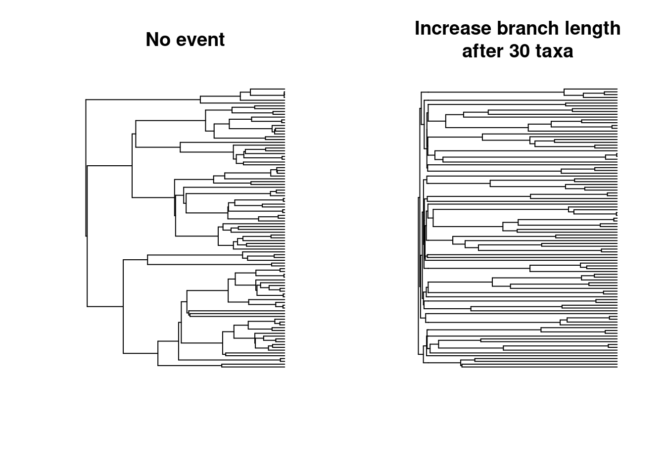

8.9 Founding event: generating a subtree with no fossils

For this scenario, we want to generate a birth-death tree for 4 time units. After reaching 10 taxa, one random taxa will give birth to a sub-tree that is a pure birth tree (no extinction).

First we need to set up the simulation parameters: * The stopping rule (5 time units) * The birth-death parameters (speciation rate of 1 and extinction of 0.2)

## Set up parameters
stop_time_4 <- list(max.time = 4)
spec_1_ext_02 <- make.bd.params(speciation = 1, extinction = 0.2)

And our event which triggers after reaching 10 taxa (taxa.condition(10)), and generates a subtree (“founding”) that is a pure birth tree (no extinction and speciation rate of 2).

## Setting the pure-birth parameters
speciation_2 <- make.bd.params(speciation = 2)

## Events that generate a new process (founding effects)
founding_event <- make.events(
                  condition = taxa.condition(10),
                  target  = "founding",
                  modification = founding.event(
                                    bd.params = speciation_2),
                  additional.args = list(prefix = "founding_"))

Note we are prodviding an additional argument prefix here so that we can track which species are part of the sub tree for colouring them down the line.

Once these parameters are defined, we can run the simulations and plot the results:

## Simulations
set.seed(11)
founding_tree <- treats(stop.rule = stop_time_4,
                      bd.params = spec_1_ext_02,
                      events = founding_event)

## Selecting the edges colours
tip_values <- rep("black", Ntip(founding_tree))
tip_values[grep("founding_", founding_tree$tip.label)] <- "orange"
edge_colors <- match.tip.edge(tip_values, founding_tree, replace.na = "black")

## Plotting the results
plot(founding_tree, show.tip.label = FALSE, edge.color = edge_colors)

8.10 Founding event: generating a subtree a different process

For this scenario, we want to generate a birth-death tree with a one dimensional Brownian Motion trait for 6 time units. After a taxon reaches the value 3 or higher, it gives birth to a sub-tree that generates an OU trait with a long-term mean at the value 3.

First we need to set up the simulation parameters: * The stopping rule (6 time units) * The birth-death parameters (speciation rate of 1 and extinction of 1/3)

## The tree parameters
stop_time_6 <- list(max.time = 6)
speciation_1_extinction_03 <- make.bd.params(speciation = 1,
                                             extinction = 0.3)

Then set up our trait which is a one dimensional Brownian Motion

## Trait
simple_bm_trait <- make.traits(n = 1, process = BM.process)

When a taxa reaches the value 3 trait.condition, it generates a pure birth tree (speciation = 2) with an OU trait with the long-term mean value 3.

## The OU trait with a long-term mean value of 3
OU_3 <- make.traits(process = OU.process,
                    start = 3, process.args = list(optimum = 3))
## The pure birth parameters
speciation_2 <- make.bd.params(speciation = 2)

## The founding event
new_OU_trait <- make.events(
                    condition    = trait.condition(3, condition = `>=`),
                    target       = "founding",
                    modification = founding.event(
                                    bd.params = speciation_2,
                                    traits    = OU_3))

Once these parameters are defined, we can run the simulations and plot the results:

## Simulating the tree
set.seed(1)
founding_tree <- treats(stop.rule = stop_time_6,
                      bd.params = speciation_1_extinction_03,
                      traits = simple_bm_trait,
                      events = new_OU_trait)
plot(founding_tree)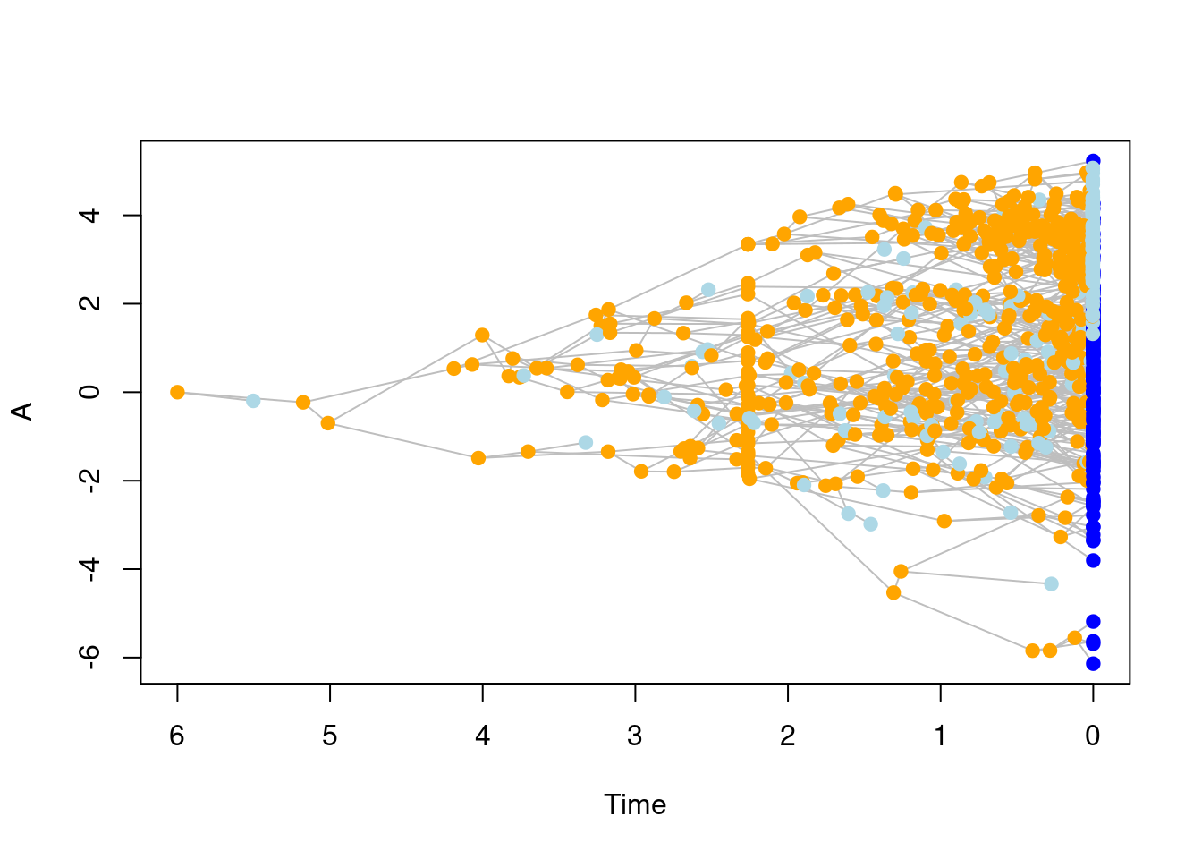

Beck, Robin MD, and Michael SY Lee. 2014. “Ancient Dates or Accelerated Rates? Morphological Clocks and the Antiquity of Placental Mammals.” Proceedings of the Royal Society B: Biological Sciences 281 (1793): 20141278.

Guillerme, Thomas, Mark N Puttick, Ariel E Marcy, and Vera Weisbecker. 2020. “Shifting Spaces: Which Disparity or Dissimilarity Measurement Best Summarize Occupancy in Multidimensional Spaces?” Ecology and Evolution 10 (14): 7261–75.