7 Plots

"treats" objects can be directly plotted in treats using the S3 plot.treats function (or just plot(x) if x is of class "treats").

7.1 Plotting traits

"treats" "traits" objects are covered in the traits section. You can use plot.treats to plot them by choosing which specific trait to plot using the trait argument (default is 1):

## Making a list of three traits
list_of_traits <- make.traits(process = c(no.process, BM.process, OU.process),
                              trait.names = c("No process (normal)", "Brownian motion", "Ornstein-Uhlenbeck"))
## Plotting each trait separately
par(mfrow = c(2, 2))
plot(list_of_traits, trait = 1)
## Using different colours options
plot(list_of_traits, trait = 2, col = c("red", "purple", "pink"))
## Not using the default plot name
plot(list_of_traits, trait = 3, main = "OU process",
     cent.tend = sd, quantiles = c(10, 30))
par(mfrow = c(1, 1))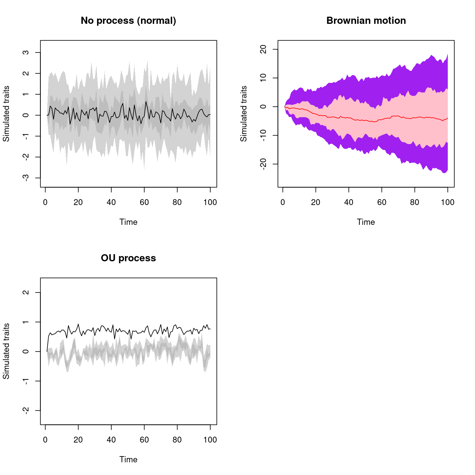

You can also control the number of replicates in the simulation by using the simulations option (the default is 50). Bigger numbers lead to more time but smoother looking plots while smaller ones are more stochastic:

par(mfrow = c(2,1))
plot(list_of_traits, trait = 2, simulations = 10, main = "10 BM simulations")
plot(list_of_traits, trait = 2, simulations = 1000, main = "1k BM simulations")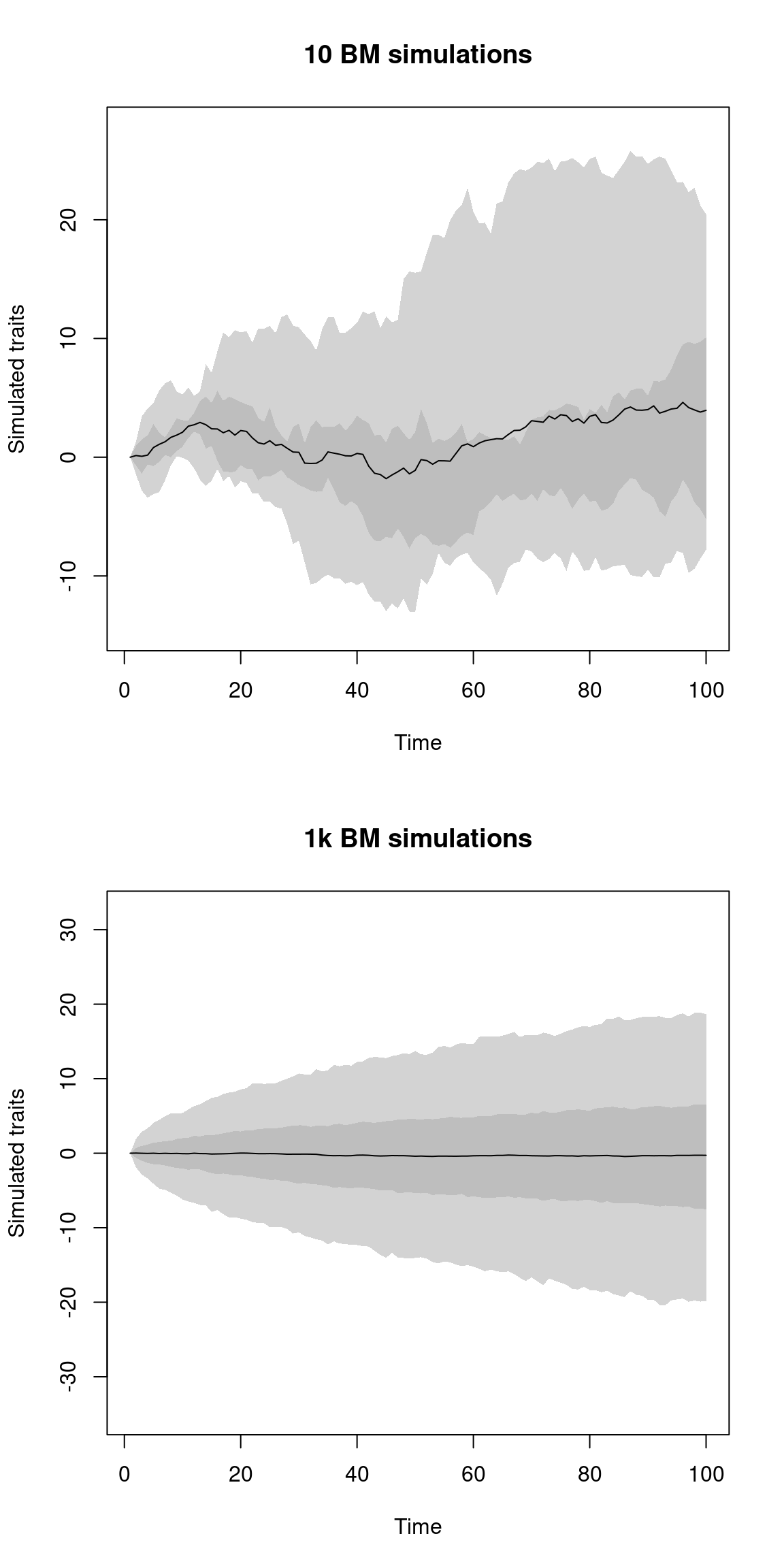

par(mfrow = c(1,1))

7.2 Plotting treats results

If treats is used to plot only a tree (and outputs a "phylo" object), you can use the function plot.phylo from the ape package to plot your tree. You’ll find all the tree plotting options in the ?plot.phylo manual page.

## A simple pure birth tree
my_tree <- treats(stop.rule = list(max.taxa = 20))
plot(my_tree, main = "Plotting a \"phylo\" object")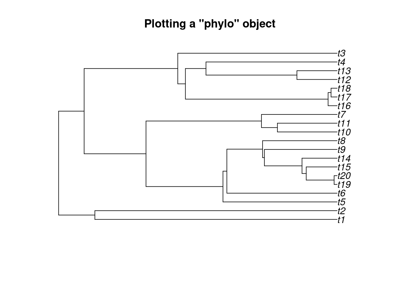

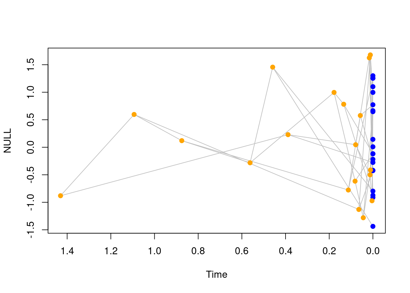
However, if you also simulated a trait along with the tree you can use the plot.treats function to plot both the tree and the trait:

## A simple pure birth tree with a BM process
my_tree <- treats(stop.rule = list(max.taxa = 20), traits = make.traits())
## Playing with the default options
plot(my_tree, main = "A tree and traits")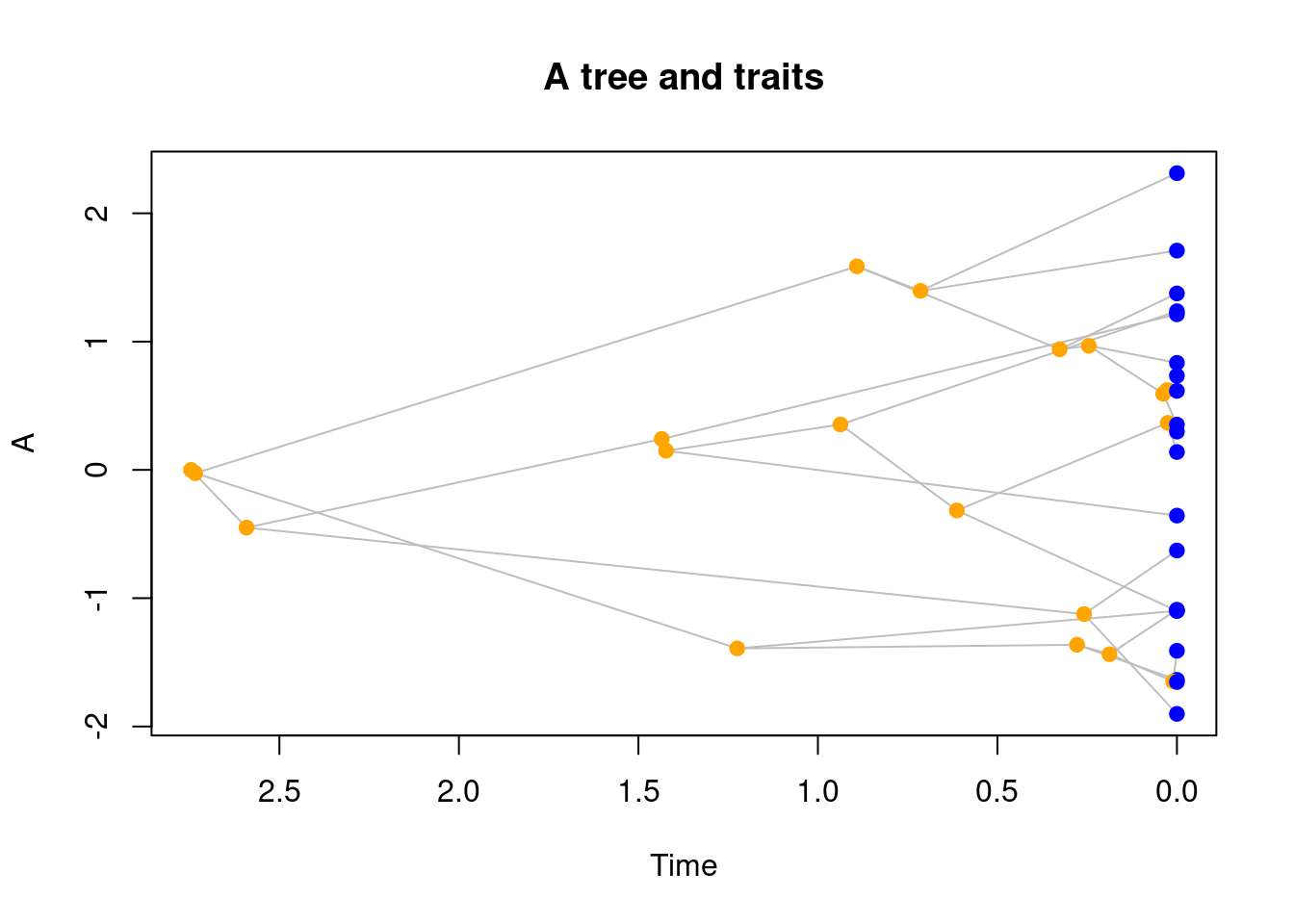

By default, elements are coloured as follows: nodes and tips are points and coloured in blue if they are tips (light blue if they are fossils) and nodes are in orange. Branches linking them are grey lines. You can of course change this colour palette to whatever you prefer by calling the standard base R arguments that can be passed to points or lines. For example pch for the point type or lty for the line type. Furthermore, time is plotted conventionally from left to right (left is towards the past, right is towards the present) but you can change that by specifying xlim.

## Playing with some more options
plot(my_tree, main = "A tree and traits",
     ## Changing nodes colours and type
     col = c(tips = "pink", nodes = "purple"), pch = 21,
     ## Changing edge colour and type
     lwd = 2, lty = 3, edges = "yellow",
     ## Changing the x axis orientation and label
     xlim = c(0, 2.5), xlab = "Time into the past")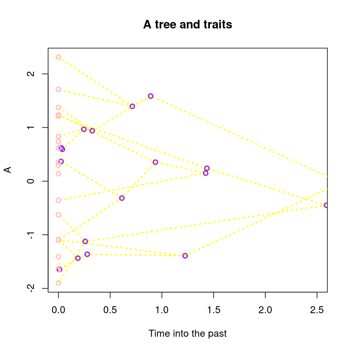

Note that in plot.treats you can modify colours using the col argument by providing a clear indication of what you want to colour (e.g. col = c(tips = "blue", fossils = "orange") will apply the colours to the unambiguously named elements) or by providing a function that will scale the colours with time (e.g. col = grDevices::heat.colors will use the specified function to change the colours of the elements through time).

You can add a default legend by using legend = TRUE (if you don’t want to add the default legend you can add it after your plot using legend(...)).

## Adding the default legend
plot(my_tree, legend = TRUE)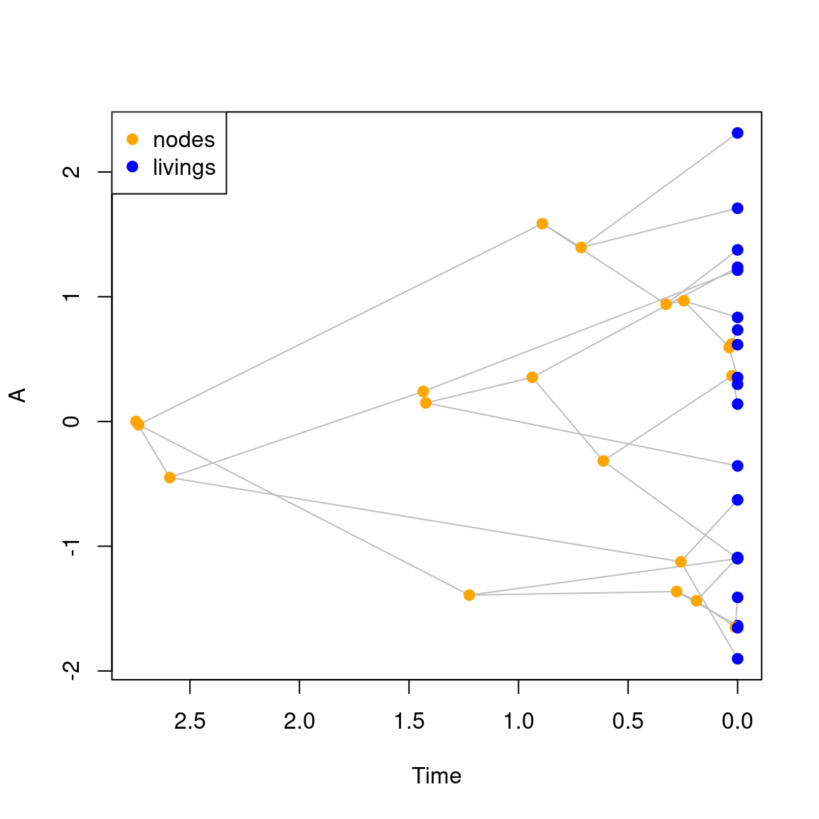

7.2.1 Adding dimensions! Not necessary, but fun!

Of course, if you’re simulating multiple traits, you can always plot different ones.

## Specifying a 3D trait process
my_3D_trait <- make.traits(n = 3)
## Simulating a birth-death tree with that 3D trait
my_data <- treats(bd.params  = list(extinction = 0.2),
                  stop.rule  = list(max.living = 50),
                  traits     = my_3D_trait,
                  null.error = 100)

## Building the tree:..Done.

You can toggle which trait to plot using the trait option, either by providing a single value to plot that specific trait against time or by providing two traits.

par(mfrow = c(2,1))
## Plotting the second trait
plot(my_data, trait = 2, main = "Trait 2")
## Plotting the correlation between trait 1 and 2
plot(my_data, trait = c(1,2), main = "Traits 1 and 2")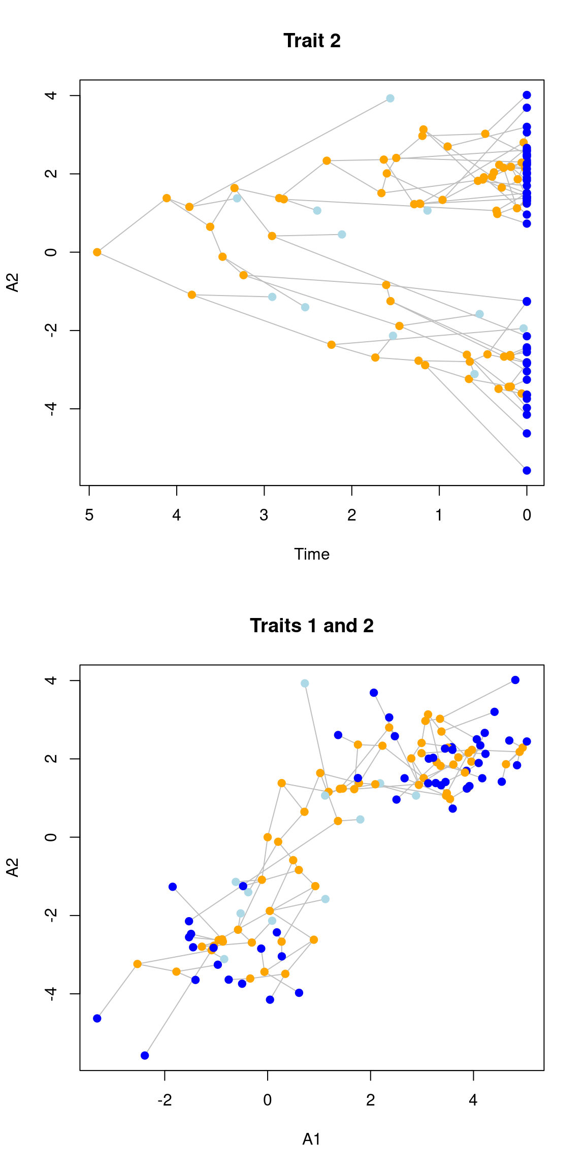

As mentioned above, the col argument can take a function for scaling the elements colours with time. This can be useful for adding time a third dimension to these 2D plots:

## Plotting the correlation between trait 1 and 2
## with time as a 3rd dimensions
plot(my_data, trait = c(1,2), main = "Traits 1 and 2",
     col = grDevices::heat.colors, legend = TRUE,
     ## Highlighting the tips in black for visibility
     tips.nodes = "black")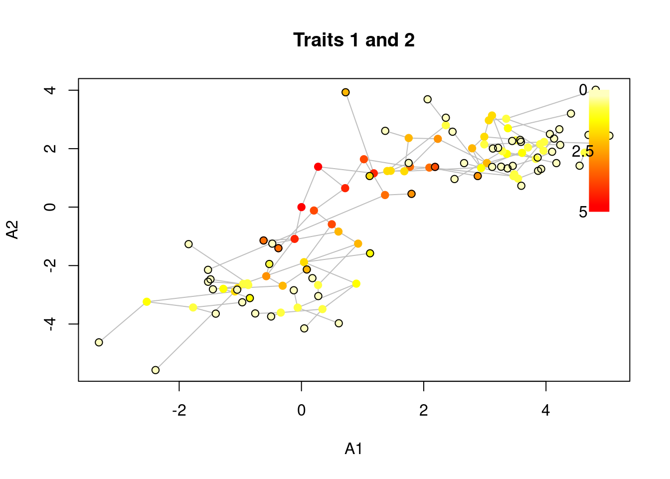

But there’s more! You can also plot these results using actual 3D plots that you can spin and all that! This is done through the rgl package and activated in treats using the option use.3D = TRUE.

If two traits are provided, the 3rd dimension is going to be time by default:

## Plotting the tree and 2 traits in 3D: woah!
plot(my_data, trait = c(1, 2), use.3D = TRUE)
rglwidget()

If three traits are provide, you can set up a fourth coloured dimension as time (similarly to the 2D plots with the colour gradients). This uses the rgl functions, namely lines3d, points3d (if type = "p"; default) or sphere3d (if type = "s"). The additional arguments ... are directly handled and attributed to the corresponding function.

## Plotting the tree and 3 traits in 3D
plot(my_data, trait = c(1, 2, 3), use.3D = TRUE,
     col = grDevices::heat.colors, type = "s", radius = 0.1)
rglwidget()

7.3 Using plot.treats to plot non-treats objects

If you like the plotting style of treats trees and data, you can always use the make.treats function to plot a tree and some traits as a "treats" object. If you have a dataset that contains trait data for tips and nodes you can transform it into a "treats" object and plot it using the generic plot.treats function:

set.seed(1)
## Generating some random tree
my_tree <- makeNodeLabel(rcoal(20))

## Generating some random discrete data
discrete_data <- sample(c(1,2), 39, replace = TRUE)
names(discrete_data) <- c(my_tree$tip.label, my_tree$node.label)

## Creating a treats object with this data
discrete_treats <- make.treats(tree = my_tree, data = discrete_data)

## Plot the data together
plot(discrete_treats, legend = TRUE)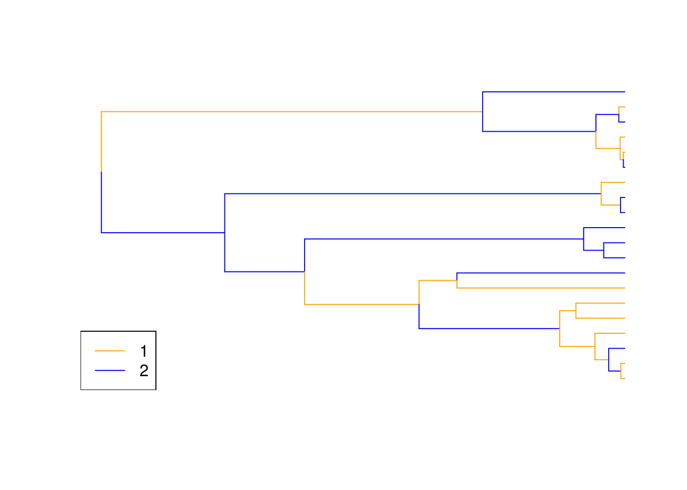

The same goes for continuous data:

## Generating some random continuous data
continuous_data <- rnorm(39)
names(continuous_data) <- c(my_tree$tip.label, my_tree$node.label)

## Creating a treats object with this data
continuous_treats <- make.treats(tree = my_tree, data = continuous_data)

## Plot the data together
plot(continuous_treats)