2 Getting started
2.1 The simplest analysis: simulating diversity only
One of the simplest things to do with the treats package is to simulate a birth-death tree.
For that you can use the function treats and specify your stopping rule.
The stopping rule simply tells the birth-death process to stop whenever it reaches one of these three conditions:
"max.taxa" = nstop whenntaxa are generated;"max.living" = nstop when there arenco-occuring taxa of the same age (i.e. “living” taxa);"max.time" = nstop when the simulated tree isnunits of age old (these units are arbitrary);
For example, we might want to generate a birth-death tree with 20 taxa:
## Setting a stopping rule to reach a maximum of 20 taxa
my_stop_rule <- list(max.taxa = 20)
We can now run the simulations using:
## Running the birth-death simulation
my_tree <- treats(stop.rule = my_stop_rule)
Note that here we could have specified more than one stopping rule, for example, we might want to run a simulation and stop it if it either reaches 10 taxa or the age 2 using
stop.rule = list(max.time = 2, max.taxa = 10). The simulation will then stop when either of these conditions are met.
The resulting object is a classic "phylo" object that you can plot like so:
## The tree object
my_tree
##
## Phylogenetic tree with 20 tips and 19 internal nodes.
##
## Tip labels:
## t1, t2, t3, t4, t5, t6, ...
## Node labels:
## n1, n2, n3, n4, n5, n6, ...
##
## Rooted; includes branch lengths.## Plotting it
plot(my_tree)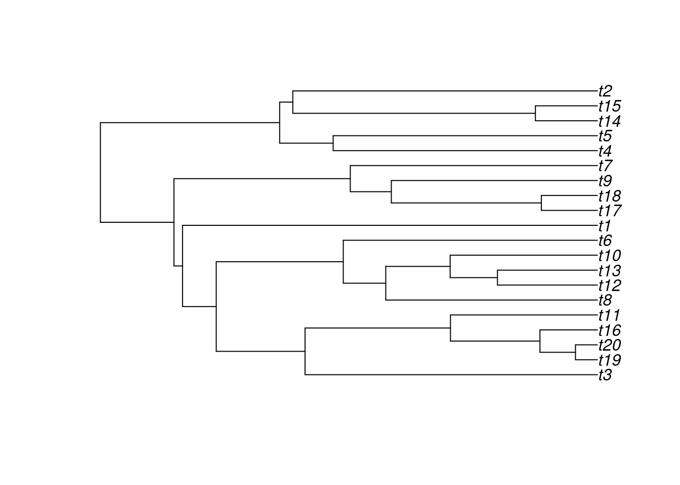
2.1.1 Changing the birth-death parameters
People familiar with the birth-death models might have noticed that we did not specify two important things here: the speciation parameter (sometimes called “lambda” or “birth”) and the extinction parameter (sometimes called “mu”, “death” or “background extinction”).
By default treats runs a pure birth model (speciation is set to 1 and extinction to 0).
However, you can easily change that by specifying your own birth-death parameters:
## my birth-death parameters
my_params <- list(speciation = 1,
extinction = 1/3)You can find more information about setting up more complex birth-death parameters in this section.
You can then run the same birth-death tree simulation with extinction:
## Generating a birth-death tree with extinctions:
my_tree <- treats(bd.params = my_params, stop.rule = my_stop_rule)
## Visualising the new tree
plot(my_tree)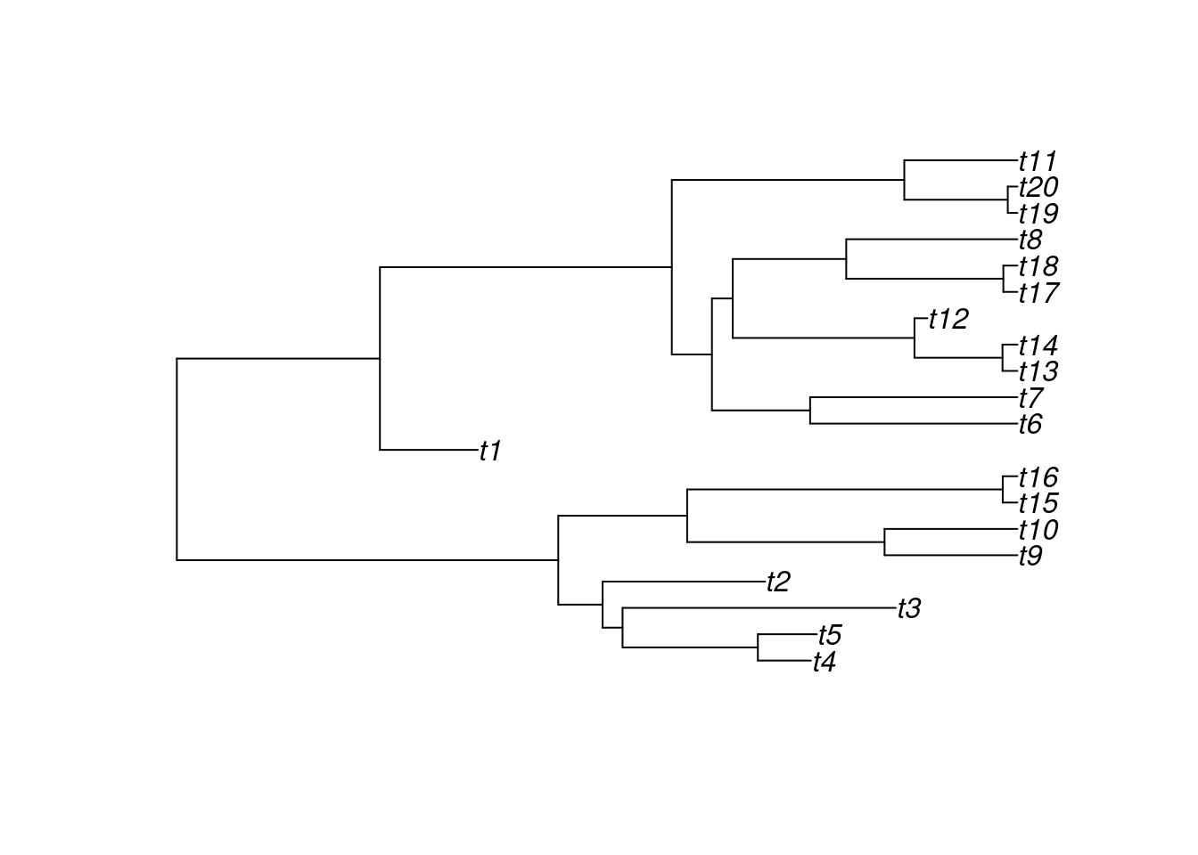
2.2 Slightly more complex: simulating disparity and diversity
Chances are that you are using treats because you also want to simulate traits (disparity) along with your diversity (otherwise, we suggest using the TreeSim package that provides many more birth-death models).
Simulating traits is not much more complicated in treats: you’ll simply need to create a "traits" object using the make.traits function.
These objects can have increasing complexity (see the rest of this tutorial) but we will keep it simple here.
"traits" objects contain one or more processes which are the ways to generate the trait.
The most common of these processes is the Brownian Motion model.
This is used by default with the make.traits function:
## Creating the traits object
my_trait <- make.traits()This trait object can be simply printed (to see what’s in it) or plotted (to see what the process looks like in the absence of a phylogeny):
## Which process is in here?
my_trait## ---- treats traits object ----
## 1 trait for 1 process (A) with one starting value (0).## What does it look like?
plot(my_trait)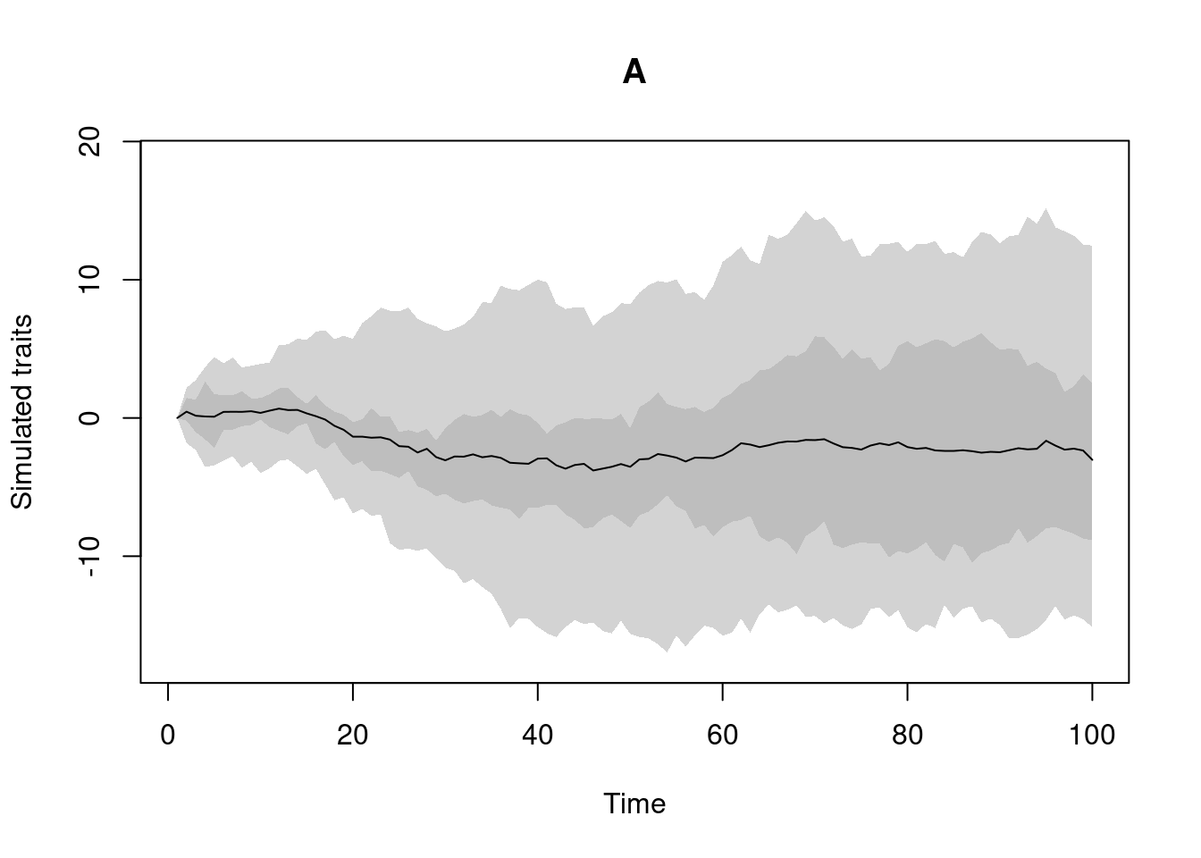
By default, this trait is called “A”.
This is not a really good name but you’ll see more about specifying trait names later on.
If this is what the process should look like (theoretically) you can then add its "traits" object to our previous treats function to generate the tree and the traits:
## Simulate disparity and diversity
set.seed(43)
my_data <- treats(bd.params = my_params,
stop.rule = my_stop_rule,
traits = my_trait)Et voilà! We now have a simple disparity and diversity simulation. We can see what’s in the results by simply printing it or plotting it:
## What's in there
my_data## ---- treats object ----
## Simulated phylogenetic tree (x$tree):
##
## Phylogenetic tree with 20 tips and 19 internal nodes.
##
## Tip labels:
##   t1, t2, t3, t4, t5, t6, ...
## Node labels:
##   n1, n2, n3, n4, n5, n6, ...
##
## Rooted; includes branch lengths.
##
## Simulated trait data (x$data):
## 1 trait for 1 process (A) with one starting value (0).## Plotting the disparity and diversity
plot(my_data)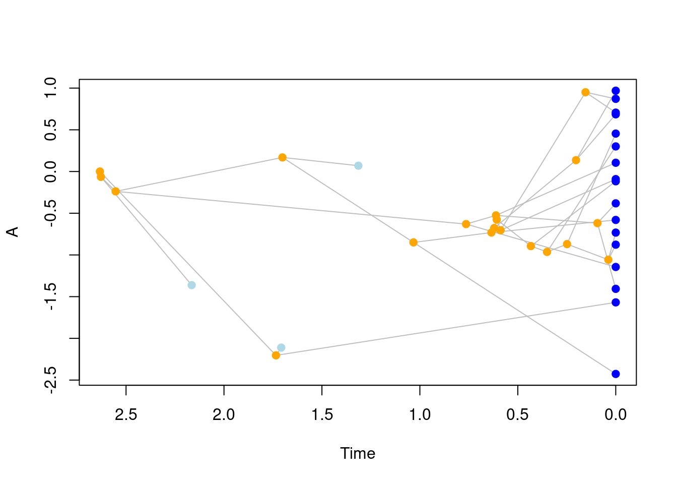
You can then extract the components you need for your specific analysis like so:
## Extracting the tree
the_generated_tree <- my_data$tree
# Note that this is a "phylo" object
class(the_generated_tree)
## [1] "phylo"## Extracting the data
the_generated_data <- my_data$data
# Note that this is a "matrix" or "array"
class(the_generated_data)## [1] "matrix" "array"You can find much more about how to design trait objects in the make.traits section.
2.2.1 "treats" objects
treats will output either just a tree (class "phylo") if no traits were generated or a "treats" object that contains both a $tree ("phylo") and a $data ("matrix") component.
Note that this "treats" class is generalised to most outputs of the package functions.
This allows for a smoother handeling of the objects outputs such as summarising the content of a make.bd.params output or visualising a trait output from make.traits.
2.3 Slightly more complex again: simulating linked disparity and diversity
The example above is still pretty simple and easily done through a variety of R packages: here the trait and the tree are simulated at the same time but only the tree is simulating the trait (i.e. the trait value at a tip is affected by its ancestor and the branch length leading to it) but not the other way around (the trait value does not affect the tree).
It is possible to add this aspect using "modifiers" objects.
"modifiers" are similar to "traits" in that you specify what should go in there and then feed it to your simulation.
"modifiers" affect two key steps of the birth-death process: the calculation of the waiting time (i.e. the component generating branch lengths) and the triggering of speciation or extinction events.
These events can be modified using condition and modify functions.
In other words, when reaching a certain condition specified by a condition function, the birth-death process will modify either the branch length or the speciation (or extinction) probability by applying a modify function.
You can use the function make.modifiers to design a specific "modifiers" object.
By default, this function generates a "modifiers" object that affects branch length and speciation in the following way:
- branch length is a randomly drawn number from an exponential distribution with a rate equal to the current number of taxa multiplied by the sum of the speciation and extinction rates.
- speciation is triggered if a randomly drawn number (from a (0,1) uniform distribution) is smaller than the ratio between the speciation rate and the sum of the speciation and extinction rates. If that random number is greater, the lineage goes extinct.
Note that these are defaults for a birth-death tree and were already applied in the examples above without specifying a "modifiers" object:
## Make a default modifiers object
default_modifiers <- make.modifiers()
## What's in it?
default_modifiers
## ---- treats modifiers object ----
## No modifiers applied to the branch length, selection and speciation processes (default).This will not do anything to our simulations compared to the previous trait and tree simulation but we can provide our "modifiers" object to the treats function:
## Setting the simulation parameters
extinction_02 <- list(extinction = 0.2)
living_20     <- list(max.living = 20)
BM_trait      <- make.traits()

# Set random seed so we get the same results
set.seed(1)

## Simulate disparity and diversity
default_data <- treats(bd.params = extinction_02,
                       stop.rule = living_20,
                       traits    = BM_trait,
                       modifiers = default_modifiers)
default_data
## ---- treats object ----
## Birth death process with modifiers:
## speciation: 1.
## extinction: 0.2.
## No modifiers applied to the branch length, selection and speciation processes (default).
## Simulated phylogenetic tree (x$tree):
##
## Phylogenetic tree with 24 tips and 23 internal nodes.
##
## Tip labels:
## t1, t2, t3, t4, t5, t6, ...
## Node labels:
## n1, n2, n3, n4, n5, n6, ...
##
## Rooted; includes branch lengths.
##
## Simulated trait data (x$data):
## 1 trait for 1 process (A) with one starting value (0).Note however, that the printing information is now updated to state that you’ve added a "modifiers" object (even though it’s the same as the default).
In this specific case the modifiers object is not necessary as it is doing nothing different than when using the default one (i.e. when no modifiers is provided).
For more interesting simulations however, you can provide modifiers that actually modify the birth-death process.
We can create one for example that makes species go extinct if their ancestor has a negative trait value.
For that we need to create a "modifiers" object that modifies the speciation process with a specific condition and a specific modification when that condition is met.
For a speciation to occur (and a species to not go extinct), the algorithm draws a random value x between 0 and 1 and if the value is smaller than the speciation parameter divided by the speciation + extinction parameter, the lineage speciates (\(x < (\lambda \div (\lambda + \mu))\)), else it goes extinct.
x is a random value that simulates some stochasticity in the evolutionary simulation.
At every step of the simulation, a different random value x is drawn making sure that the resulting speciation or extinction is not predictable.
However, we can create a modifier that introduces less randomness (or a different level of randomness) by forcing the lineage to go extinct every time a specific condition is met, e.g. if the lineage trait value is negative. This can be done for example by not randomly generating the value x but giving it a fixed value of say 1 so that the estimation of the speciation function \(x < (\lambda \div (\lambda + \mu))\) is always met. In other words, if the lineage’s trait value is negative, make sure that x is equal to 1, so that the speciation condition \(x < (\lambda \div\ (\lambda + \mu))\) is never met.
First we need to create a condition function to trigger this (non) speciation event.
We can do that by specifying our condition function (here the going.extinct function) to apply our modification.
For that we can use the parent.traits utility function that is optimised for accessing traits in the birth-death process (but you can of course write your own).
This function takes the trait.values and parent.lineage arguments, two arguments that you can leave named as they are to facilitate treats’ understanding of what you want to assess:
## Triggering a modification only if the ancestor trait is negative
negative.ancestor <- function(trait.values, lineage) {
    return(all(parent.traits(trait.values, lineage) < 0))
}
Note that we use the function
allhere to evaluate all traits: i.e. if the data has more than one trait we trigger the modification only if all the trait values are negative.
Then we create the modification function.
This function must take the argument x and, in our case, returns the same value no matter what: 1 so that speciation never happens when the negative.ancestor function is triggered.
## Always go extinct
going.extinct <- function(x) return(1)
This going.extinct function is to be contrasted with the normal modifier for selecting the value x which is runif(1) (drawing a random value between 0 and 1).
We can then provide these two functions (the condition negative.ancestor and how to modify the speciation event when this condition is met going.extinct).
If you are an advances treats user, you can design your own speciation function but if you just want to use a normal speciation function, you can use the default one from treats called speciation.
## Making a modifier for species to go extinct if
## their ancestor's trait value is (or are) negative
negatives_extinct <- make.modifiers(
            ## If the following condition is met...
            condition = negative.ancestor, # Does the lineage have an ancestor with negative trait values?
            ## Then apply the following modifier...
            modify = going.extinct, # The species goes extinct
            ## To the the speciation process.
            speciation = speciation) # Here the speciation() process is default

## What's in it?
negatives_extinct
## ---- treats modifiers object ----
## Default branch length process.
## Default selection process.
## Speciation process is set to speciation with a condition (negative.ancestor) and a modifier (going.extinct).Note that the make.modifiers function tests whether the input is compatible with treats by default so unless you have an error message, your modifiers will work!
We can now simulate our tree and traits with our modifier: species will go extinct if their ancestor has a negative trait value:
set.seed(1)
## Simulate disparity and diversity
modified_data <- treats(bd.params = extinction_02,
                        stop.rule = living_20,
                        traits    = BM_trait,
                        modifiers = negatives_extinct)
modified_data
## ---- treats object ----
## Birth death process with modifiers:
## speciation: 1.
## extinction: 0.2.
## Default branch length process.
## Default selection process.
## Speciation process is set to speciation with a condition (negative.ancestor) and a modifier (going.extinct).
## Simulated phylogenetic tree (x$tree):
##
## Phylogenetic tree with 22 tips and 21 internal nodes.
##
## Tip labels:
## t1, t2, t3, t4, t5, t6, ...
## Node labels:
## n1, n2, n3, n4, n5, n6, ...
##
## Rooted; includes branch lengths.
##
## Simulated trait data (x$data):
## 1 trait for 1 process (A) with one starting value (0).We can now compare the two trees and their trait values.
Note that we’ve used the same starting seed for both trees so the only thing differing between them is the "modifier" object which leads to very different trees!
par(mfrow = c(1,2))
plot(default_data, main = "default results")
plot(modified_data, main = "results with the modifier")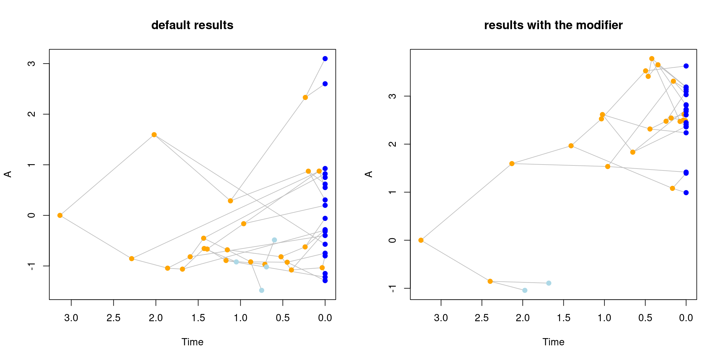
You can find much more about how to design modifiers in the make.modifiers section.
2.4 An illustrative example: mammals disparity through the K-Pg extinction
Bib is studying the evolution of mammalian disparity (i.e. diversity of shapes) across the Cretaceous-Palaeogene mass extinction event (K-Pg - 66 million years ago).
They use a dataset from Beck and Lee (2014) that is a discrete morphological space containing the ordination of the around 400 morphological characters for 50 species and estimated for their 49 descendants into an ordinated shapespace of 99 elements and 97 dimensions.
library(dispRity)
## Loading the mammalian morphological example data
data(BeckLee_mat99)

## This is what the dataset looks like
head(BeckLee_mat99)[1:5, 1:5]
## [,1] [,2] [,3] [,4] [,5]
## Cimolestes -0.6794737 0.15658591 0.04918307 0.2250983 -0.38139436
## Maelestes -0.5797289 0.04223105 -0.20329542 -0.1545388 -0.06993258
## Batodon -0.8812102 0.33619889 0.41748560 0.2446872 -0.31922156
## Bulaklestes -0.9295090 -0.08517626 0.11364659 0.3589646 -0.54998508
## Daulestes -1.0025229 -0.09260779 0.06354371 0.4614256 -0.61211569And a tree showing the relation between these species through time:
## The phylogenetic tree
data(BeckLee_tree)

## And what the tree looks like
plot(BeckLee_tree, cex = 0.8)
axisPhylo()
abline(v = BeckLee_tree$root.time - 66, col = "red")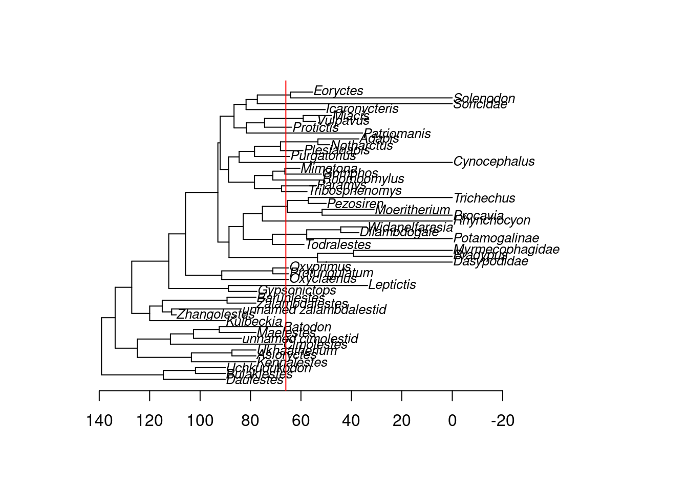
They measure the disparity as the sum of variances as a proxy for changes in the traitspace size (Guillerme et al. (2020)) with some bootstrapping to create some confidence intervals around that curve.
## Making continuous time series
time_series <- chrono.subsets(data = BeckLee_mat99,
                              tree = BeckLee_tree,
                              method = "continuous", model = "proximity",
                              time = seq(from = 101, to = 41, by = -5))
## Calculating disparity
change_in_size <- dispRity(boot.matrix(time_series), metric = c(sum, variances))
plot(change_in_size)
abline(v = 8, col = "red")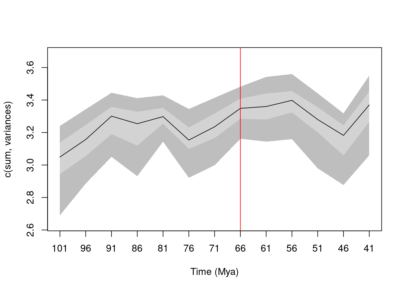
For more info about
chrono.subsetsand thedispRitypackage, you can have a look at thedispRitymanual.
Looking at this curve, Bib wants to know whether disparity increased as a response to the K-Pg mass extinction or not. To do this, they need to check whether changes in disparity can actually be detected due to an extinction event (e.g. if an extinction event happens, does that change disparity curves?). As a subsidiary question, they want to know whether the pattern is more likely due to a selective or random extinction event.
2.4.1 Simulating trees and traits using the observed parameters
The first step is to simulate the observed tree. We can do that by using crude parameters from the observed tree:
## Extracting the crude parameters
(est_params <- crude.bd.est(BeckLee_tree, method = "count"))
## ---- treats birth-death parameters object ----
## speciation: 0.028.
## extinction: 0.027.## These parameters are the observed speciation and extinction rate per million years.
## Setting the stopping rule (stop after reaching 50 taxa)
stop_rule <- list(max.taxa = 50)
## Simulating just a birth-death tree with these parameters to check
set.seed(1)
test_tree <- treats(bd.params = est_params,
stop.rule = stop_rule,
null.error = 100)## Building the tree:.Done.plot(ladderize(test_tree), cex = 0.8)
axisPhylo()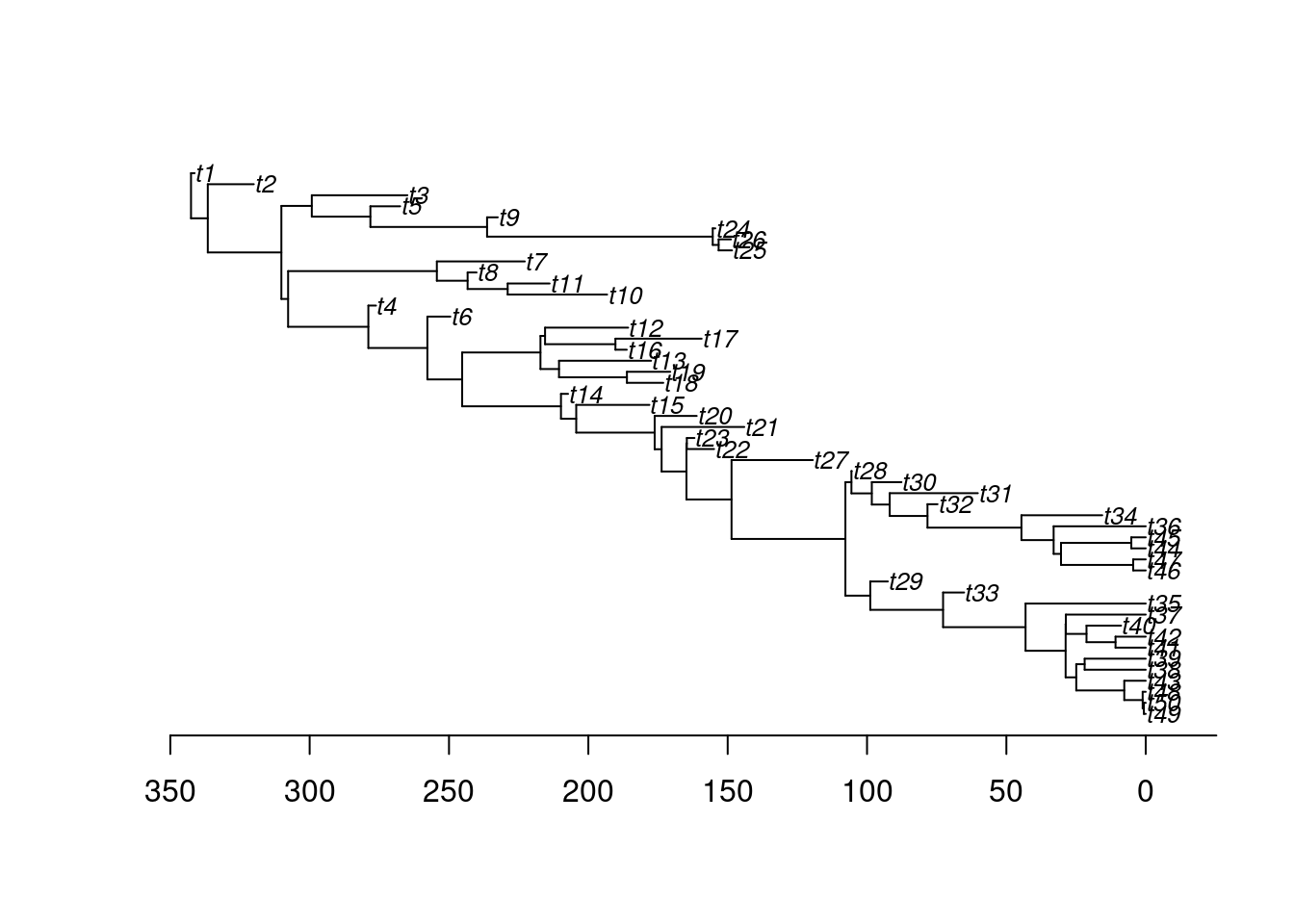
Note that because of the high extinction to speciation ratio, the tree simulations can often fail before reaching the stop rule (i.e. all lineages go extinct before reaching 50 taxa). To avoid getting stuck in there, we use the option
null.error = 100to rerun the simulations up to 100 times before obtaining a tree that did not went fully extinct. Also note that using such parameters make the simulations run slowlier but ensure the requested results are always achieved.
We now have a way to simulate a topology close to the observed one. We can simulate a list of topologies by replicating this function X amounts of time to get a distribution of trees:
## Generating 50 trees
tree_distribution <- treats(bd.params  = est_params,
                            stop.rule  = stop_rule,
                            null.error = 100,
                            replicates = 50)
Of course, here our objective is to also simulate some trait values to measure disparity under some simulated scenario.
We can do that be adding a "traits" object to the treats function.
Here we will use a default Brownian Motion to simulate our trait.
## Creating a trait in 97 dimensions.
my_traits <- make.traits(process = BM.process, n = ncol(BeckLee_mat99))
Note that there are many more options on how to simulate your trait such as using correlation, different processes, etc… See details in the make traits section.
## Simulate the tree and traits
sim_data <- treats(traits     = my_traits,
                   bd.params  = est_params,
                   stop.rule  = stop_rule,
                   null.error = 100)
We can visualise the resulting tree using the plot function and visualising the different traits using the trait option in plot:
## Plotting the results (first trait)
plot(sim_data, trait = 1)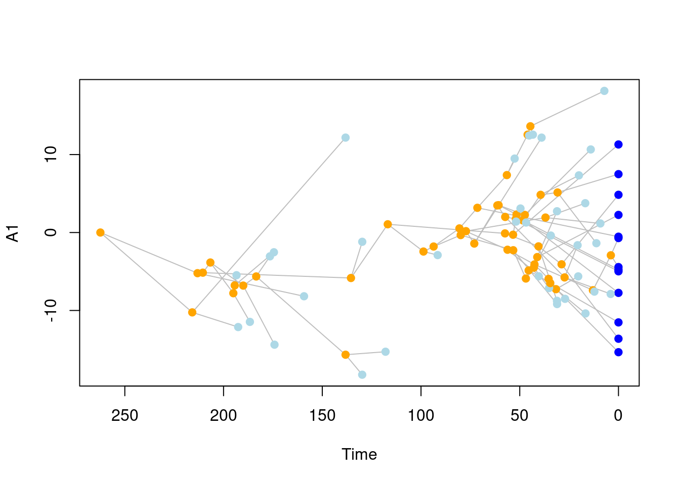
Of course, here we want to simulate a distribution of trees and traits:
## Simulate the tree and traits
sim_data <- treats(traits     = my_traits,
                   bd.params  = est_params,
                   stop.rule  = stop_rule,
                   null.error = 100,
                   replicates = 50)
Et voila! We now have a distribution of 50 trees and 50 datasets from which we can calculate disparity.
We can directly pass the results to the dispRity package pipeline using the dispRitreats function:
## Calculate the dispRity for all the simulations
simulated_disparity <- dispRitreats(sim_data,
                                    method = "continuous",
                                    model  = "proximity",
                                    time   = 10,
                                    metric = c(sum, variances),
                                    scale.trees = TRUE)
par(mfrow = c(1,2))
plot(simulated_disparity, main = "simulated disparity")
plot(change_in_size, main = "observed disparity")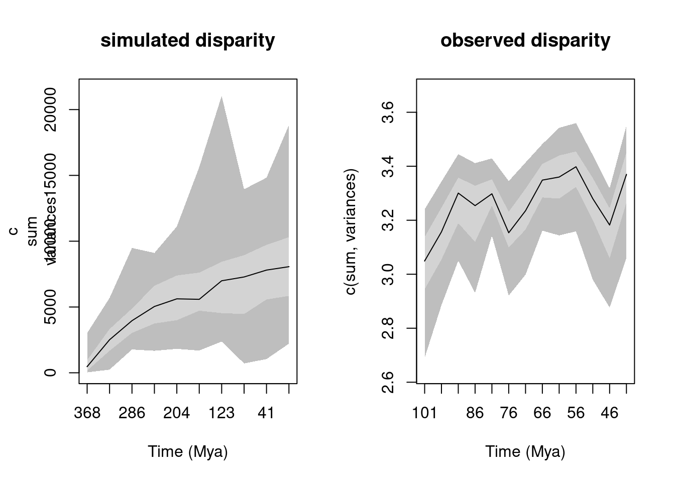
We can see that both simulated and observed disparity curves are different. From there one could already reasonably propose that the observe disparity does not entirely follows our parametrised scenario (constant speciation and extinction and BM trait evolution).
However, we can complexify our scenario to introduce the effect of mass extinction event. We can simulate two alternative scenarios: * one where we create a random extinction event after having simulated half of the species (25) where we remove 75% of species; * and a second one where we remove all the species with negative values. This allows us to simulate two contrasted scenarios to see whether using our observed dataset it would be possible to detect changes in disparity due to mass extinctions.
To do so, we need to create two mass extinction "event" objects:
## Creating a random mass extinction
random_extinction <- make.events(target = "taxa",
                                 condition = taxa.condition(25, condition = `>=`),
                                 modification = random.extinction(0.75))
## Creating an extinction that removes species with negative trait values
negative_extinction <- make.events(target = "taxa",
                                   condition = taxa.condition(25, condition = `>=`),
                                   modification = trait.extinction(x = 0, condition = `>=`))
We can then feed these two extinction events to our previous simulations
## Simulate the tree and traits with a random extinction event
sim_rand_extinction <- treats(
                   traits     = my_traits,
                   bd.params  = est_params,
                   stop.rule  = stop_rule,
                   events     = random_extinction,
                   null.error = 100,
                   replicates = 50)

## Simulate the tree and traits with a random extinction event
sim_trait_extinction <- treats(
                   traits     = my_traits,
                   bd.params  = est_params,
                   stop.rule  = stop_rule,
                   events     = negative_extinction,
                   null.error = 100,
                   replicates = 50)

## Visualising the difference between both scenarios
par(mfrow = c(1,2))
plot(sim_rand_extinction[[1]], main = "Random extinction")
plot(sim_trait_extinction[[1]], main = "Negative extinction")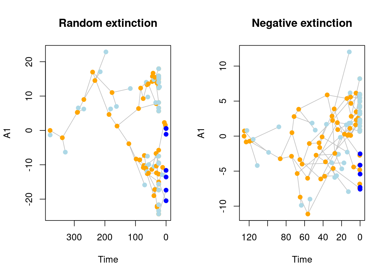
We can then measure the disparity from these scenarios and compare them to our observed ones
## Simulate the tree and traits with a random extinction event
sim_rand_extinction <- treats(
                   traits     = my_traits,
                   bd.params  = est_params,
                   stop.rule  = stop_rule,
                   events     = random_extinction,
                   null.error = 100,
                   replicates = 50)
## Building the tree:....................Done.
## Building the tree:....Done.
## Building the tree:...........Done.
## Building the tree:.Done.
## Building the tree:............Done.
## Building the tree:.Done.
## Building the tree:.Done.
## Building the tree:.Done.
## Building the tree:..............Done.
## Building the tree:...................................Done.
## Building the tree:......................Done.
## Building the tree:........Done.
## Building the tree:...................Done.
## Building the tree:...Done.
## Building the tree:.......Done.
## Building the tree:.....Done.
## Building the tree:....................Done.
## Building the tree:.Done.
## Building the tree:...Done.
## Building the tree:................Done.
## Building the tree:.......Done.
## Building the tree:.................Done.
## Building the tree:.....Done.
## Building the tree:.................Done.
## Building the tree:............Done.
## Building the tree:....Done.
## Building the tree:....Done.
## Building the tree:...Done.
## Building the tree:...................................................Done.
## Building the tree:...............Done.
## Building the tree:....Done.
## Building the tree:.........Done.
## Building the tree:..................................Done.
## Building the tree:.....Done.
## Building the tree:........Done.
## Building the tree:....Done.
## Building the tree:.Done.
## Building the tree:...................Done.
## Building the tree:...........Done.
## Building the tree:...........Done.
## Building the tree:...........Done.
## Building the tree:.Done.
## Building the tree:...........Done.
## Building the tree:.Done.
## Building the tree:.............Done.
## Building the tree:.............Done.
## Building the tree:........Done.
## Building the tree:.............Done.
## Building the tree:...Done.
## Building the tree:.Done.## Simulate the tree and traits with a random extinction event
sim_trait_extinction <- treats(
traits = my_traits,
bd.params = est_params,
stop.rule = stop_rule,
events = negative_extinction,
null.error = 100,
replicates = 50)## Building the tree:......................Done.
## Building the tree:...Done.
## Building the tree:..................Done.
## Building the tree:.......Done.
## Building the tree:.................Done.
## Building the tree:...Done.
## Building the tree:..................Done.
## Building the tree:....................Done.
## Building the tree:.Done.
## Building the tree:............Done.
## Building the tree:.Done.
## Building the tree:.Done.
## Building the tree:......Done.
## Building the tree:...............Done.
## Building the tree:....Done.
## Building the tree:.................Done.
## Building the tree:.........Done.
## Building the tree:....Done.
## Building the tree:.....Done.
## Building the tree:....Done.
## Building the tree:......Done.
## Building the tree:.....................Done.
## Building the tree:.................Done.
## Building the tree:.Done.
## Building the tree:....Done.
## Building the tree:...Done.
## Building the tree:...........................Done.
## Building the tree:.......Done.
## Building the tree:.......Done.
## Building the tree:.....Done.
## Building the tree:......Done.
## Building the tree:.......Done.
## Building the tree:.........Done.
## Building the tree:.....Done.
## Building the tree:...Done.
## Building the tree:...................Done.
## Building the tree:............Done.
## Building the tree:......................Done.
## Building the tree:......Done.
## Building the tree:............Done.
## Building the tree:.............Done.
## Building the tree:...........Done.
## Building the tree:..Done.
## Building the tree:.........................Done.
## Building the tree:.Done.
## Building the tree:......................Done.
## Building the tree:.............Done.
## Building the tree:...Done.
## Building the tree:...............Done.
## Building the tree:..........Done.## Visualising the difference between both scenarios
par(mfrow = c(1,2))
plot(sim_rand_extinction[[1]], main = "Random extinction")
plot(sim_trait_extinction[[1]], main = "Negative extinction")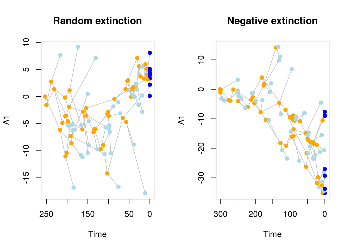
Interestingly, with all our parameters used here and our specific disparity metric we cannot detect the effect of a mass extinction.
References
Beck, Robin MD, and Michael SY Lee. 2014. “Ancient Dates or Accelerated Rates? Morphological Clocks and the Antiquity of Placental Mammals.” Proceedings of the Royal Society B: Biological Sciences 281 (1793): 20141278.
Guillerme, Thomas, Mark N Puttick, Ariel E Marcy, and Vera Weisbecker. 2020. “Shifting Spaces: Which Disparity or Dissimilarity Measurement Best Summarize Occupancy in Multidimensional Spaces?” Ecology and Evolution 10 (14): 7261–75.