3 Simulating traits

In treats, traits are simulating by providing a traits object to the traits argument. This object is generated using make.traits. In treats a trait designate any coherent character of any number of dimensions which may or may not be independent of other traits. For example, it can be a uni-dimensional variable uncorrelated to other traits or a multi-dimensional one with different amounts of correlation.

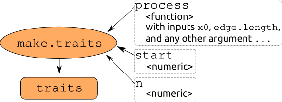
make.traits: The main inputs are (1) the process, one or more functions to describe the trait(s) as a function of previous state (x0) and the branch length (edge.length), (2) n the number of dimensions of the trait and (3) the starting value start.

3.0.1 Quick overview

function	arguments	input	what does it do
`make.traits`	process*	a function	simulates the trait (see below)
`make.traits`	n	a numeric value	the number of dimensions
`make.traits`	start	one or more numeric values	the starting values for each dimensions
`make.traits`	process.args	…	anything to be passed to `process` (see below)
`make.traits`	trait.names	a character string	the name(s) of the trait(s)
`make.traits`	add	a `treats` object	another trait generated by `make.traits`
`make.traits`	update	a `treats` object	another trait generated by `make.traits`
`make.traits`	test	logical	whether to test the validity of the trait
`make.traits`	background	a `treats` object	another trait generated by `make.traits` (to run in the background)
———	———–	——-	—————-
`process`	x0	a numeric value	the value of the previous trait
`process`	edge.length	a numeric value	the branch length value
`process`	…	…	any other argument to be handled by the process

* non-optional arguments

3.1 The process (`process`)

The function make.traits allows you to design the process of a trait or a set of traits. Here, the process of a trait designates the rules needed to generate the trait through time while simulating a phylogeny. This process can depend on the previous state in the tree (i.e. the trait of the ancestor) and the branch length to the descendant. One classic example is the Brownian motion process (or Weiner process). Note that it can depend on both the ancestor and the branch length but does not necessarily need to, i.e. the process can be based only on the previous state or only on branch length or on neither.

3.1.1 The syntax (how to code a process?)

Trait processes in treats are functions that must always take the following arguments by default.

x0: the previous trait value(s)
edge.length: the branch length
...: a placeholder for any extra arguments

For example, the following function would be a valid process that always generate the true trait value: 42!. In this example, the process is not dependent on either the previous state (x0) or the branch length (edge.length).

## A valid (but useless?) process
valid.process <- function(x0 = 0, edge.length = 1, ...) {
    return(42)
}

Note that in this function definition the arguments x0 and edge.length have a default value of 0 and 1 respectively. In practice, these arguments are effectively set to the correct values in the treats internal function (i.e. whatever x0 and edge.length are at that specific time of the process) but providing a default can help speed up the algorithms (specifically all the internal checks).

On the other hand, the following process (a unidimensional Brownian motion) is incorrect (it’s missing edge.length and ...):

## A wrongly formatted process
invalid.process <- function(x0 = 0) {
    return(rnorm(1, mean = x0))
}

This will not work in make.traits (see below).

3.1.2 Using a `"process"` in `treats`

You can design your own process as a function, as long as it has a valid syntax. Alternatively, the treats package has several inbuilt processes, namely a multidimensional Brownian motion (BM.process) or a multidimensional Ornstein-Uhlenbeck process (OU.process). You can find the list of implemented processes by looking at the ?trait.process manual page in R.

Once a process is chosen, you can feed it into the make.traits function:

## Creating a trait object
my_trait_object <- make.traits(process = BM.process)

This creates "treats" "traits" objects that you can print and visualise using the plot function:

## The class of the object
class(my_trait_object)

## [1] "treats" "traits"

## What's in it?
my_trait_object

##  ---- treats traits object ---- 
## 1 trait for 1 process (A) with one starting value (0).

## What does the process looks like
plot(my_trait_object)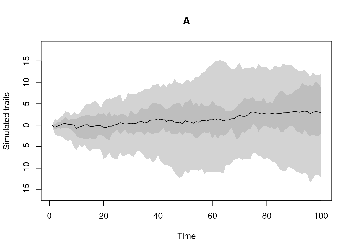

Note that you can see the multiple options for plotting the trait process by looking at ?plot.treats manual. Furthermore, you can look at what’s actually in the object using this specific syntax (this applies to every object handled by the treats package):

## What's actually in that object?
print.treats(my_trait_object, all = TRUE)

## $main
## $main$A
## $main$A$process
## $main$A$process[[1]]
## function (x0 = 0, edge.length = 1, Sigma = diag(length(x0)), 
##     ...) 
## {
##     return(t(MASS::mvrnorm(n = 1, mu = x0, Sigma = Sigma * edge.length, 
##         ...)))
## }
## <bytecode: 0x5bdff95336a8>
## <environment: namespace:treats>
## 
## 
## $main$A$start
## [1] 0
## 
## $main$A$trait_id
## [1] 1
## 
## 
## 
## $background
## NULL

As traits can get more and more complex, the automatic printing of its summary allows for a easier display of what’s in the "traits" object.

Note that it is possible to make "traits" objects with multiple traits and multiple processes (that can be the same or different for each trait):

## Four traits: two BM, one OU and one normal non process
four_traits <- make.traits(process = c(BM.process,
                                       BM.process,
                                       OU.process,
                                       no.process))
four_traits

##  ---- treats traits object ---- 
## 4 traits for 4 processes (A, B, C, D) with one starting value (0).

You can visualise them individually using the trait argument in plot.treats:

## Plot options (4 plots in one window)
par(mfrow = c(2,2))
plot(four_traits, trait = 1)
plot(four_traits, trait = 2)
plot(four_traits, trait = 3)
plot(four_traits, trait = 4)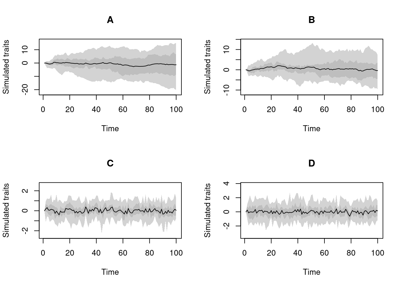

par(mfrow = c(1,1))

3.2 The number of traits `n` and the starting values `start`

Two further important arguments are n the number of traits per process and start the starting values for all traits. By default they are set to n = 1 and start = 0. This means that make.traits will assume that your processes are always unidimensional by default and that they always start with the value 0. It is possible however, to change these values.

For example you can use the following to create a three dimensional Brownian motion with each dimension starting with the value 1:

## Multidimensional Brownian motion
make.traits(BM.process, n = 3, start = 1)

##  ---- treats traits object ---- 
## 3 traits for 1 process (A:3) with one starting value (1).

Or the following with each dimensions starting with different values (respectively 1, 2 and 3):

## Multidimensional Brownian motion
make.traits(BM.process, n = 3, start = c(1,2,3))

##  ---- treats traits object ---- 
## 3 traits for 1 process (A:3) with different starting values (1,2,3).

Note that the number of traits are applied for each process by default. However, you can apply different number of traits for different processes:

## two 3D processes (BM and OU)
make.traits(c(BM.process, OU.process), n = 3)

##  ---- treats traits object ---- 
## 6 traits for 2 processes (A:3, B:3) with one starting value (0).

## one 1D processes (BM) and one 4D process (OU)
make.traits(c(BM.process, OU.process), n = c(1, 4))

##  ---- treats traits object ---- 
## 5 traits for 2 processes (A:1, B:4) with one starting value (0).

And starting values are distributed for all the traits or for the traits one by one:

## two 3D processes (BM and OU) starting with 1
make.traits(c(BM.process, OU.process), n = 3, start = 1)

##  ---- treats traits object ---- 
## 6 traits for 2 processes (A:3, B:3) with one starting value (1).

## two 3D processes (BM and OU) starting with values 1 to 6
make.traits(c(BM.process, OU.process), n = 3, start = 1:6)

##  ---- treats traits object ---- 
## 6 traits for 2 processes (A:3, B:3) with different starting values (1,2,3,4,5,6).

## two 3D processes (BM and OU) with the two first ones starting
## with 1 and the 4 other ones with the default (0)
make.traits(c(BM.process, OU.process), n = 3, start = c(1,1))

## Warning in make.traits(c(BM.process, OU.process), n = 3, start = c(1, 1)): Only
## the first 2 starting values were supplied for a required 6 traits. The missing
## start values are set to 0.

##  ---- treats traits object ---- 
## 6 traits for 2 processes (A:3, B:3) with different starting values (1,1,0,0,0,0).

3.2.1 What is a trait in `treats`?

Because it would be impossible to accommodate all definitions of a trait in treats we chose an arbitrary one: a trait is whatever you define as a trait! A trait can be uni-dimensional as the measurement of a feature of an organism (e.g. leaf surface, femur length, etc.) but can also be a multi-dimensional description of a feature, for example in 3D geometric morphometric context, a trait could be defined as “position of landmark X” (which will be a trait with three dimensions, x, y and z) or in ecology, the location of a plant can be expressed as latitude and longitude coordinates. In treats, the process corresponds to this trait definition (e.g. a process can be of n-dimensions and represents one organisms feature) and the traits represents the number of dimensions in total. So in the examples above, this is how the following traits are interpreted by treats:

## Three traits with one process:
make.traits(BM.process, n = 3, start = c(1,2,3))
## Six traits with two processes:
make.traits(c(BM.process, OU.process), n = 3)
## Five traits with two processes
make.traits(c(BM.process, OU.process), n = c(1, 4))

3.3 Multidimensional traits and correlations

As shown in the example above, a trait can be made multidimensional by using the n argument specifically passed to a process. However, in this case, traits are simulated independently of each other. It is possible to include correlation by designing a multidimensional trait process directly generating the correlation between within the dimensions of the process. Alternatively, the inbuilt BM.process and OU.process can intake a correlation matrix to simulate traits independtly but with a correlation coefficient (see this illustration with an event).

3.4 Extra argument for the processes with `process.args`

You can also feed extra arguments to your process(es) functions. For example, the inbuilt process no.process (that is just a number generator not based on the previous value x0 or the branch length) can take a specific random number generator as a function:

## no process trait using the normal distribution (default)
make.traits(no.process, process.args = list(fun = rnorm))

##  ---- treats traits object ---- 
## 1 trait for 1 process (A) with one starting value (0).
## process A uses the following extra argument: fun.

## no process trait using the uniform distribution
## bounded between 1 and 100
make.traits(no.process, process.args = list(fun = runif, min = 1, max = 100))

##  ---- treats traits object ---- 
## 1 trait for 1 process (A) with one starting value (0).
## process A uses the following extra argument: c("fun", "min", "max").

You can also add multiple extra arguments for multiple processes giving them as a list.

## Two traits with no process:one normal and one uniform (1,100)
make.traits(process = c(no.process, no.process),
            process.args = list(list(fun = rnorm),
                                list(fun = runif, min = 1, max = 100)))

##  ---- treats traits object ---- 
## 2 traits for 2 processes (A, B) with one starting value (0).
## process A uses the following extra argument: fun.
## process B uses the following extra argument: c("fun", "min", "max").

If one process does not need extra argument you must still give it an extra NULL process argument:

## Three traits with no process:
## one default, one lognormal and one uniform (1,100)
make.traits(process      = c(no.process, no.process, no.process),
            process.args = list(## Extra arguments for the first process (none)
                                list(NULL),
                                ## Extra arguments for the second process
                                list(fun = rlnorm),
                                ## Extra arguments for the third process
                                list(fun = runif, min = 1, max = 100)))

##  ---- treats traits object ---- 
## 3 traits for 3 processes (A, B, C) with one starting value (0).
## process B uses the following extra argument: fun.
## process C uses the following extra argument: c("fun", "min", "max").

3.5 Naming the traits with `trait.names`

As traits become more and more complex, it can be useful to give clearer names to each process. This is easily done using the trait.names argument that attributes one name per process:

## A simple trait with a proper name
simple_trait <- make.traits(trait.names = "1D Brownian Motion")
simple_trait

##  ---- treats traits object ---- 
## 1 trait for 1 process (1D Brownian Motion) with one starting value (0).

This becomes more useful if we use the complex example above:

## Three named traits with no process:
## one default, one lognormal and one uniform (1,100)
make.traits(process      = c(no.process, no.process, no.process),
            process.args = list(## Extra arguments for the first process (none)
                                list(NULL),
                                ## Extra arguments for the second process
                                list(fun = rlnorm),
                                ## Extra arguments for the third process
                                list(fun = runif, min = 1, max = 100)),
            ## Naming each trait
            trait.names  = c("Normal", "LogNormal", "Uniform(1,100)"))

##  ---- treats traits object ---- 
## 3 traits for 3 processes (Normal, LogNormal, Uniform(1,100)) with one starting value (0).
## process LogNormal uses the following extra argument: fun.
## process Uniform(1,100) uses the following extra argument: c("fun", "min", "max").

3.6 Combining multiple traits with `add`

You can also add traits to already existing trait objects using the simple add option. This option just takes a "treats" "traits" object and the additional process(es) will be added to it. For example:

## Creating a simple default Brownian motion
one_process <- make.traits(trait.names = "BM")

## Creating a new trait (a 3D OU.process)
## and adding the previous one
two_processes <- make.traits(OU.process, n = 3, add = one_process,
                             trait.names = "3D OU")

## Only one process
one_process

##  ---- treats traits object ---- 
## 1 trait for 1 process (BM) with one starting value (0).

## The two processes
two_processes

##  ---- treats traits object ---- 
## 4 traits for 2 processes (BM:1, 3D OU:3) with one starting value (0).

3.7 Using a background trait

traits objects also allow a background trait to be used when traits are simulated (step 3 here). This allows traits to be simulated for all tips whenever a trait is generated for one tip. This can be useful for keeping track of trait values along the simulation (cf just at bifurcating nodes). The background argument takes any output from the make.traits function in a nested way:

## Generating a default BM trait:
BM_trait <- make.traits()
## Generating an OU trait with a background BM trait
my_trait <- make.traits(process = OU.process, background = BM_trait)

Note that technically you can nest as many background traits as you want (e.g. make.traits(background = make.traits(background = make.traits(...))) is valid). However, you should always make sure that the background trait has the same dimensions as the main trait. When using a trait with background, your tree will have internal singleton nodes (i.e. nodes linking to one ancestor and only one descendant). You can remove these nodes using the drop.things function.

set.seed(1)
## Generating a pure birth tree with the background trait
tree_bkg <- treats(stop.rule = list(max.taxa = 20),
                   traits = my_trait)
## This tree has many internal singleton nodes
plot(tree_bkg)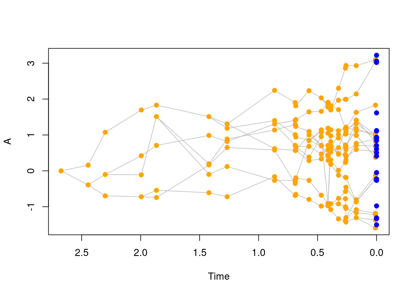

3.8 Saving trait values at different time steps

You can also simulate a tree by generating traits at specific time steps with the save.steps option in treats. This will apply the traits object to all lineages currently alive at the required time steps. These time steps can be either regular by providing a single numeric value; e.g. save.steps = 0.1 will take a snapshot of the trait values every 0.1 units of time, or specific, by providing a specific set of values; e.g. save.steps = c(1, 1.2, 3) will take a snapshot of the trait values at the required time steps.

set.seed(123)
## Generating a birth-death tree with a BM trait and saving steps at specific times
tree_steps <- treats(stop.rule  = list(max.time = 3),
                     bd.params  = list(speciation = 1, extinction = 0.1),
                     traits     = make.traits(),
                     save.steps = c(1/3, 1, 2))
## This also creates internal singleton nodes
plot(tree_steps)
abline(v = 3 - c(1/3, 1, 2), lwd = 0.5, col = "grey")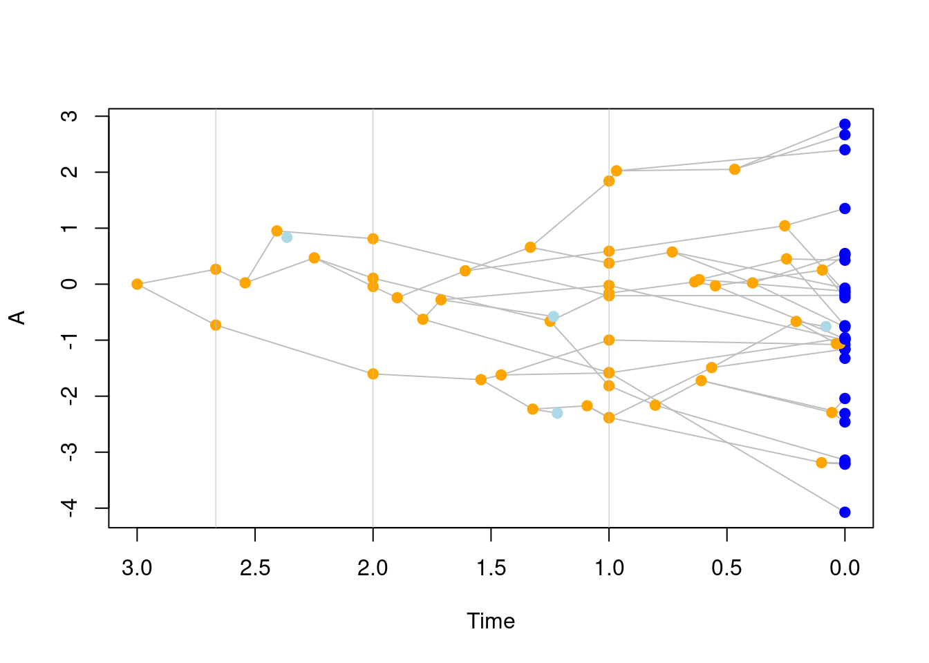

3.9 Linking traits together with `link.traits`

In the treats algorithm, traits are simulated in parallel for improving performances. Most of the cases this is a (really) good thing! However, in some cases you might need some of your traits to be simulated sequentially. For example if you want a specific trait process or options to be dependent on the result of another trait. You can set up these linked traits using the link.traits function. This function takes base.trait, a "treats" "traits" object created using make.traits that will be the first trait simulated and the next.trait, a list of "treats" "traits" objects that will be simulated after the base.trait depending on the link type (link.type) and some other arguments (link.args). So far the link.traits function only accommodates link.type = "conditional" for conditional traits.

3.9.1 Conditional traits

Say for example that you have a primary trait (base.trait) that is a discrete binary trait that generates values 0 or 1. This can correspond to some abiotic trait for example (e.g. “is the lineage on an island or on the mainland”). You can first generate this trait using the make.traits function as detailed above (note here we’re using a transition matrix as a specific argument that makes the changes from state 0 to state 1 relatively rare and the reversal even more rare).

## Setting up a discrete trait
discrete_trait <- make.traits(discrete.process,
       process.args = list(transitions = matrix(c(3, 0.2, 0.05, 3), 2, 2)),
       trait.names  = "discrete")

Following this trait value, we can create another trait that is conditional to the outcome of this first discrete trait simulation. In other words we can specify a choice between two processes depending on the result of the base.trait. For example, we can say that if the lineage evolves on an island (state "1") it will evolve using a Brownian motion process but if it evolves on the mainland (state "0"), it will evolve using an OU process.

We’ll need to first generate these two traits independently using make.traits (using different options):

## A standard Brownian Motion trait
BM_trait <- make.traits(process = BM.process)
## An OU trait with a strong alpha
OU_trait <- make.traits(process = OU.process, process.args = list(alpha = 10))
## Combining both traits into a list
continuous_trait <- list("mainland_case" = BM_trait,
                         "island_case"   = OU_trait)

We then need to create a list of functions to interpret the results of the first trait (discrete_trait) so that if the results of discrete_trait is 0, BM_trait is used, if it’s 1 OU_trait is used. This is done by creating a list of functions that evaluate x1, the outcome of discrete_trait, and return a logical (TRUE or FALSE). For example function(x1) {x1 != 0} will return TRUE if the discrete_trait is not state 0:

## Creating a list of functions to choose between either case for the continuous trait
select_continuous <- list("is.mainland" = function(x1) {x1 == 0},
                          "is.island"   = function(x1) {x1 == 1})

Note that this list must be in the same order as the continuous_trait: the functions will be evaluated sequentially (i.e. test the function is.mainland, then is.island) and the first one to return TRUE will be used to select the function in continuous_trait. For example in our case if the score of discrete_trait is 1, the second function from select_continuous is TRUE so the second element from continuous_trait is used (the OU_trait).

We can then combine all that using link.traits:

## Link these traits
conditional_trait <- link.traits(# The first trait to be evaluated
                                 base.trait = discrete_trait,
                                 # The other traits to be evaluated next
                                 # (here a list of two traits)
                                 next.trait = continuous_trait,
                                 link.type  = "conditional",
                                 # The functions to choose between either
                                 # continuous traits 
                                 link.args  = select_continuous)

And run the usual simulation pipeline with treats:

## Running a tree with this conditional trait
set.seed(123)
my_conditional_tree <- treats(stop.rule = list(max.taxa = 200),
                              traits    = conditional_trait)

op <- par(mfrow = c(1,2))
plot(my_conditional_tree, trait = 1, main = "The conditional trait")
plot(my_conditional_tree, trait = 2, main = "The conditioned trait")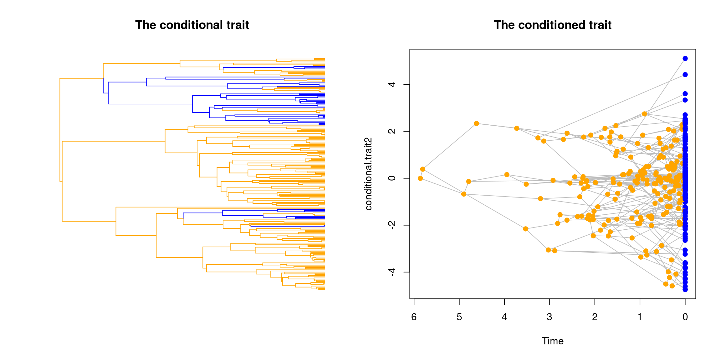

par(op)
## The clumpy bit around the value 0 corresponds to the OU trait

Of course, you can combine linked traits with other traits like any other traits in treats using make.traits (for example: make.traits(process = my_new_trait, add = conditional_trait) to generate more complex traits. In this case the traits are generated in parallel (for speed) apart for the specified linked ones.

3.10 Traits implemented in `treats`

If you don’t want to design your own trait process, you can use one of the following trait processes that are currently implemented in treats. You can find more information about their many options using their specific manuals in R or the generic ?trait.process:

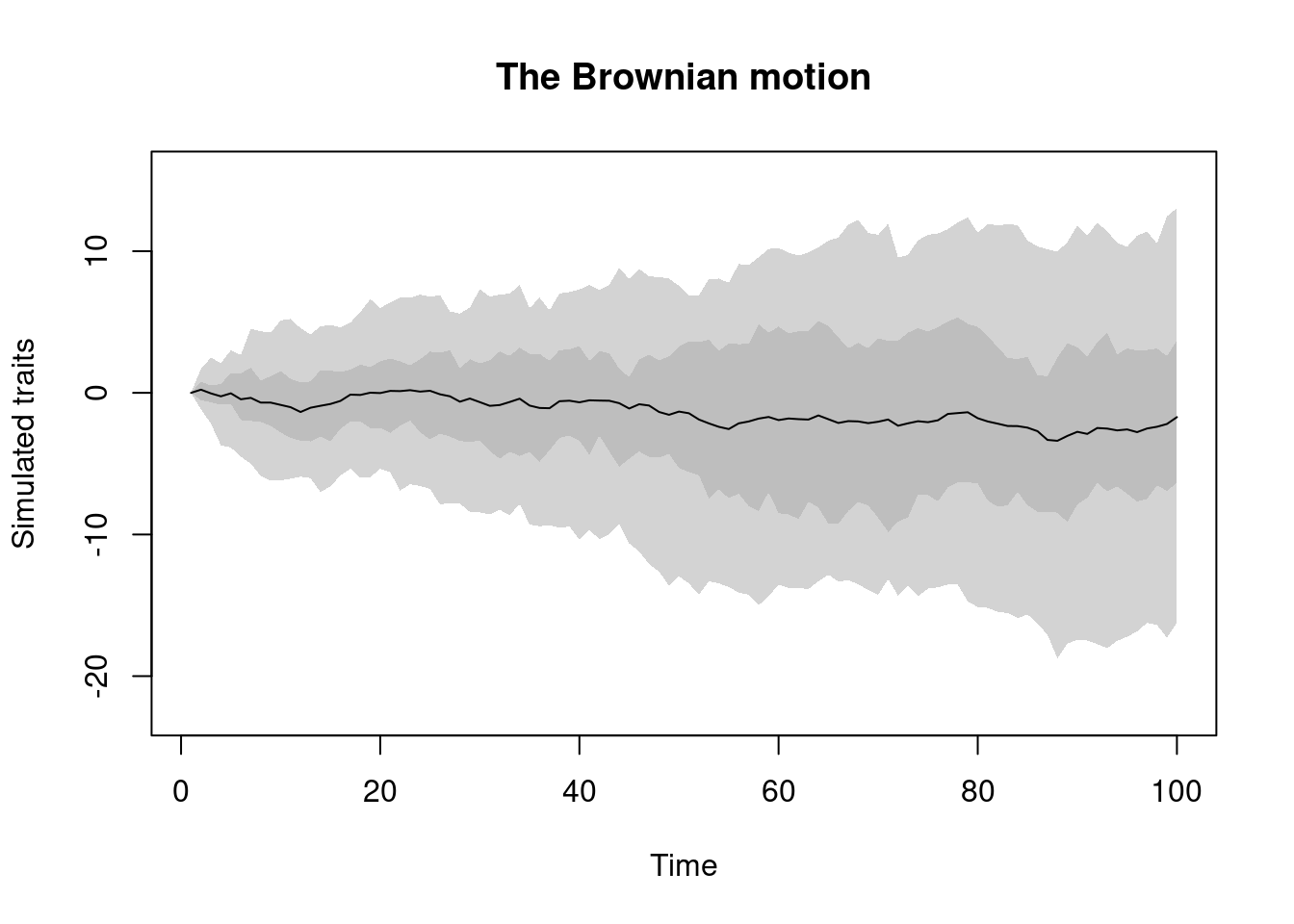
BM.process: this is the well known Brownian motion process.

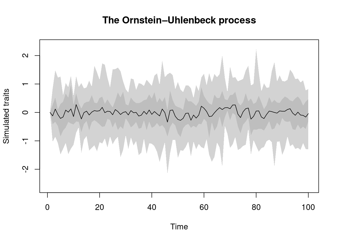
OU.process: this is the equally famous Ornstein–Uhlenbeck process.

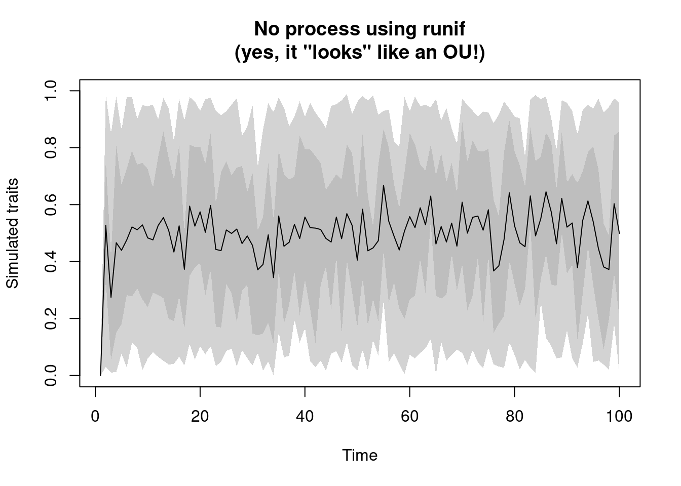
no.process: this process has… no process. In other words, this is a non time dependent process; the simulated value does not depends on the ancestors’ value nor the branch length. It’s basically a place holder for a random sampling function like rnorm (default), runif, rlnorm, etc.

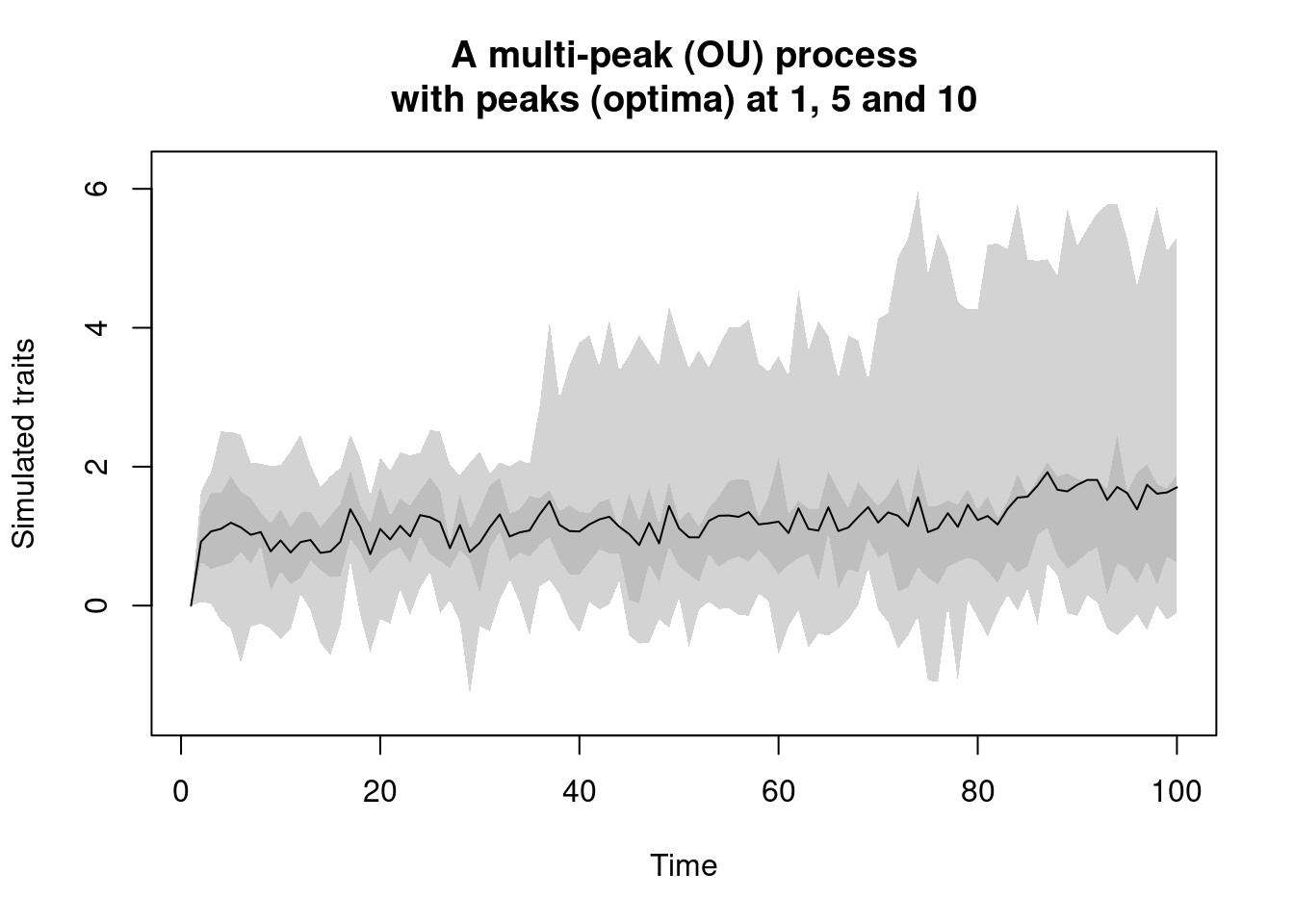
multi.peak.process: this process is a modified version of the OU.process that can take multiple local long-term mean values. The default OU process has one long-term mean towards which the values are drawn with the alpha parameter (the elastic band). The single long-term mean is usually 0. However, with this multi.peak.process we can set multiple values towards which values can be attracted with the same alpha parameter.

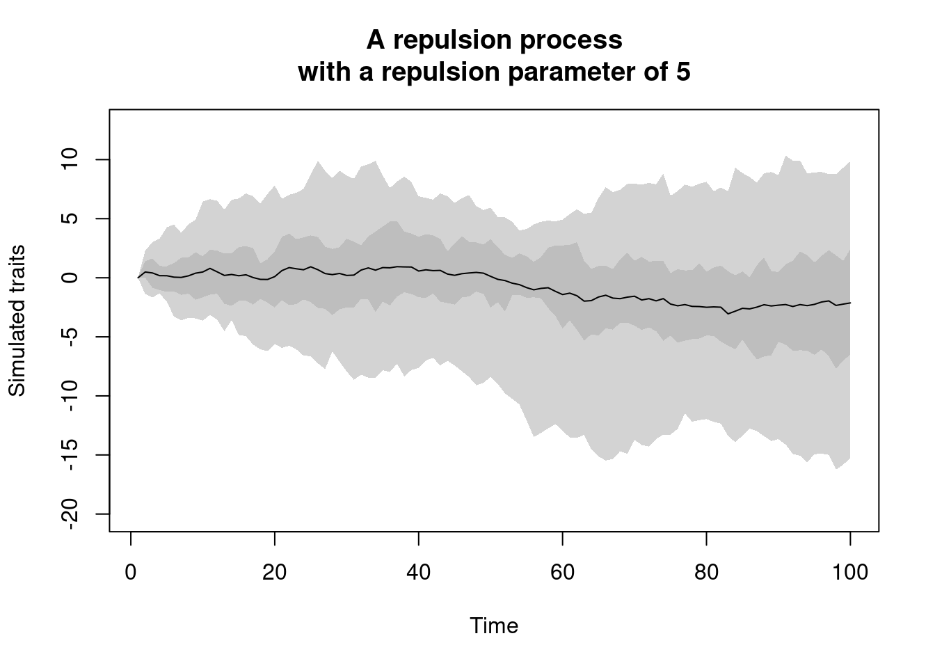
repulsion.process: this is a modified version of the BM.process where instead of accumulating gradually through time, new trait values are more likely to be different to the traits of their ancestor following a repulsion parameter.

discrete.process: this one generates discrete trait values based on a transition matrix (you can use the utility function transition.matrix to generate one).

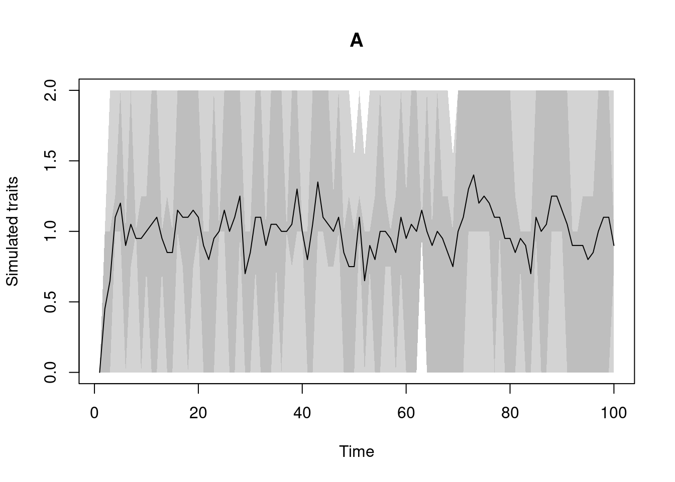
Of course here the plotting of a discrete trait is not that informative…

3.11 Testing the traits with `test`

This bit is still in development. We highly suggest leaving test = TRUE so that make.traits returns an error if a process or its additional arguments (process.args) are not formatted correctly. make.traits will send an error if the trait cannot be directly passed to treats. However, in some specific cases (again, probably mainly for development and debugging) it could be useful to skip the tests using test = FALSE.

3.12 Mapping traits on a tree: `map.traits`

Although make.traits is mainly designed for treats simulations, i.e. simulating both the trees AND the traits at the same time, it is possible to use an already simulated or estimated tree and generating one or more traits on it using the map.traits function. This function takes the trait input as a "traits" object (from make.traits) and a tree topology with branch length. Note that you can also use "traits" objects with multiple or multi-dimensional traits as well as multiple phylogenies ("multiPhylo").

## Simulating a random tree with branch length
my_tree <- rtree(20)

## Creating three different traits objects:
## A Brownian Motion
bm_process <- make.traits(process = BM.process)
## An Ornstein-Uhlenbeck process
ou_process <- make.traits(process = OU.process)
## No process (just randomly drawing values from a normal distribution)
no_process <- make.traits(process = no.process)

## Mapping the three traits on the phylogeny
bm_traits <- map.traits(bm_process, my_tree)
ou_traits <- map.traits(ou_process, my_tree)
no_traits <- map.traits(no_process, my_tree)

## Plotting the topology and the different traits
par(mfrow = c(2,2))
plot(my_tree, main = "Base topology")
plot(bm_traits, main = "Mapped BM")
plot(ou_traits, main = "Mapped OU")
plot(no_traits, main = "Mapped normal trait")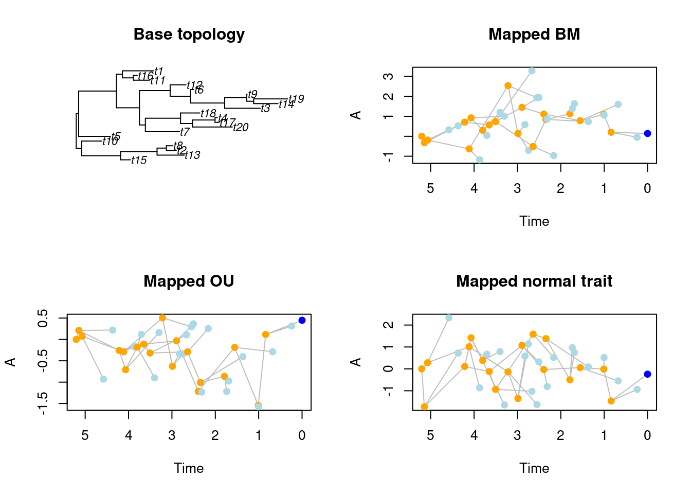

3.13 Templates for making your very own process

As detailed above, any process of your own design will work as long as it is a function that takes at least the arguments x0 and edge.length. You can be imaginative and creative when designing your own process but here are two detailed example functions for a unidimensional Brownian Motion and Ornstein-Uhlenbeck process that you can use for a start (or not). Remember it is good practice for treats processes to set all the arguments with default values (just in case).

Note that the functions below are not equal to the already implemented BM.process and OU.process but an easier to edit version that you can use as a template:

3.13.1 A simple Brownian Motion process template

## A simple Brownian motion process
my.BM.process <- function(x0 = 0, edge.length = 1, sd = 1, ...) {
    ## Drawing a random number from a normal distribution
    ## with x0 as the and a given standard deviation
    ## and depending on branch (edge) length
    result <- rnorm(n = 1, mean = x0, sd = sqrt(sd^2 * edge.length))

    ## Return the number
    return(result)
}

3.13.2 A simple Ornstein-Uhlenbeck process template

## A simple Ornstein-Uhlenbeck motion process
my.OU.process <- function(x0 = 0, edge.length = 1, var = 1, alpha = 1, ...) {
    ## Calculate the mean based on alpha
    mean <- x0 * exp(-alpha)
    ## Calculate the standard deviation based on alpha and the variance
    sd <- sqrt(var/(2 * alpha) * (1 - exp(-2 * alpha)))
    ## Draw a random number from a normal distribution
    ## using this mean and standard deviation
    ## and depending on branch (edge) length
    result <- rnorm(n = 1, mean = mean, sd = sqrt(sd^2 * edge.length))

    ## Return the number
    return(result)
}

3 Simulating traits

3.0.1 Quick overview

3.1 The process (process)

3.1.1 The syntax (how to code a process?)

3.1.2 Using a "process" in treats

3.2 The number of traits n and the starting values start

3.2.1 What is a trait in treats?