Ginzburg-Landau equation
We end this paper with the implementation of the complex Ginzburg-Landau equation, which is a nonlinear time dependent reaction-diffusion problem. The equation to solve is $$ \begin{equation} \frac{\partial u}{\partial t} = \nabla^2u + u - (1 + 1.5i)u |u|^2, \tag{62} \end{equation} $$ for the doubly periodic domain \( \Omega = [-50, 50]\times [-50, 50] \) and \( t \in [0, T] \). The initial condition is chosen as one of the following $$ \begin{align} u^0(\boldsymbol{x}, 0) &= (ix + y) \exp {-0.03 (x^2 + y^2)} \tag{63}, \\ u^1(\boldsymbol{x}, 0) &= (x + y) \exp {-0.03 (x^2 + y^2)} \tag{64}. \end{align} $$ This problem is solved with the spectral Galerkin method using Fourier bases in both directions, and a tensor product space \( W(x,y)=V^p(x) \otimes V^p(y) \), where \( V^p \) is defined as in the section Periodic boundary conditions, but here mapping the computational domain \( [-50, 50] \) to \( [0, 2\pi] \). Considering only the spatial discretization, the variational problem becomes: find \( u(x, y) \) in \( W \), such that $$ \begin{equation} \frac{\partial }{\partial t} (v, u)^N = (v, \nabla^2u)^N + (v, u - (1 + 1.5i)u |u|^2)^N \quad \text{for all} \quad v \in W, \tag{65} \end{equation} $$ and we integrate the equations forward in time using an explicit, fourth order Runge-Kutta method, that only requires as input a function that returns the right hand side of (65). Note that all matrices involved with the Fourier method are diagonal, so there is no need for linear algebra solvers, and the left hand side inner product equals \( (2 \pi)^2 \bs{\hat{u}} \).
The initial condition is created using Sympy
from sympy import symbols, exp, lambdify
x, y = symbols("x,i y")
#ue = (1j*x + y)*exp(-0.03*(x**2+y**2))
ue = (x + y)*exp(-0.03*(x**2+y**2))
ul = lambdify((x, y), ue, 'numpy')
We create a regular tensor product space, choosing the fourier.bases.C2CBasis for both directions if the initial
condition is complex (63), whereas we may choose R2CBasis if the initial condition is real
(64). Since we are solving a nonlinear equation, the additional issue of aliasing should be
considered. Aliasing errors may be handled with different methods, but here we will use the so-called 3/2-rule,
that requires padded transforms. We create a tensor product space Tp for padded transforms, using the
padding_factor=3/2 keyword below. Furthermore, some solution arrays, test and trial functions are also declared.
# Size of discretization
N = (201, 201)

# Create tensor product space
K0 = C2CBasis(N[0], domain=(-50., 50.))
K1 = C2CBasis(N[1], domain=(-50., 50.))
T = TensorProductSpace(comm, (K0, K1))

Kp0 = C2CBasis(N[0], domain=(-50., 50.), padding_factor=1.5)
Kp1 = C2CBasis(N[1], domain=(-50., 50.), padding_factor=1.5)
Tp = TensorProductSpace(comm, (Kp0, Kp1))

u = TrialFunction(T)
v = TestFunction(T)
X = T.local_mesh(True)
U = Function(T, False)         # Solution
U_hat = Function(T)            # Solution spectral space
Up = Function(Tp, False)       # Padded solution for nonlinear term
dU_hat = Function(T)           # right hand side
#initialize
U[:] = ul(*X)
U_hat = T.forward(U, U_hat)
Note that Tp can be used exactly like T, but that a backward transform creates an output that is 3/2 as large in each direction. So a \( (100, 100) \) mesh results in a \( (150, 150) \) output from a backwards transform. This transform is performed by creating a 3/2 times larger padded array in spectral space \( \hat{u}^p_{\textsf{k}^p} \), where \( \textsf{k}^p = \boldsymbol{l}^p \times \boldsymbol{l}^p \) and
$$
\begin{equation}
\boldsymbol{l}^{p} = -3N/4, -3N/4+1, \ldots, 3N/4-1.
\tag{66}
\end{equation}
$$
We then set \( \hat{u}^p_{\textsf{k}} = \hat{u}_{\textsf{k}} \) for \( \textsf{k} \in \boldsymbol{l} \times \boldsymbol{l} \), and for the remaining high frequencies \( \hat{u}^p_{\textsf{k}} \) is set to 0.
We will solve the equation with a fourth order Runge-Kutta integrator. To this end we need to declare some work arrays to hold intermediate solutions, and a function for the right hand side of Eq. (65)
U_hat0 = Function(T)
U_hat1 = Function(T)
w0 = Function(T)
a = [1./6., 1./3., 1./3., 1./6.]         # Runge-Kutta parameter
b = [0.5, 0.5, 1.]                       # Runge-Kutta parameter
def compute_rhs(rhs, u_hat, U, Up, T, Tp, w0):
    rhs.fill(0)
    U = T.backward(u_hat, U)
    rhs = inner(v, div(grad(U)), output_array=rhs, uh_hat=u_hat)
    rhs += inner(v, U, output_array=w0, uh_hat=u_hat)
    rhs /= (2*np.pi)**2  # (2pi)**2 represents scaling with inner(u, v)
    Up = Tp.backward(u_hat, Up)
    rhs -= Tp.forward((1+1.5j)*Up*abs(Up)**2, w0)
    return rhs
Note the close similarity with (65) and the usage of the padded transform for the nonlinear term. Finally, the Runge-Kutta method is implemented as
t = 0.0
dt = 0.025
end_time = 96.0
tstep = 0
while t < end_time-1e-8:
    t += dt
    tstep += 1
    U_hat1[:] = U_hat0[:] = U_hat
    for rk in range(4):
        dU_hat = compute_rhs(dU_hat, U_hat, U, Up, T, Tp, w0)
        if rk < 3:
            U_hat[:] = U_hat0 + b[rk]*dt*dU_hat
        U_hat1 += a[rk]*dt*dU_hat
    U_hat[:] = U_hat1
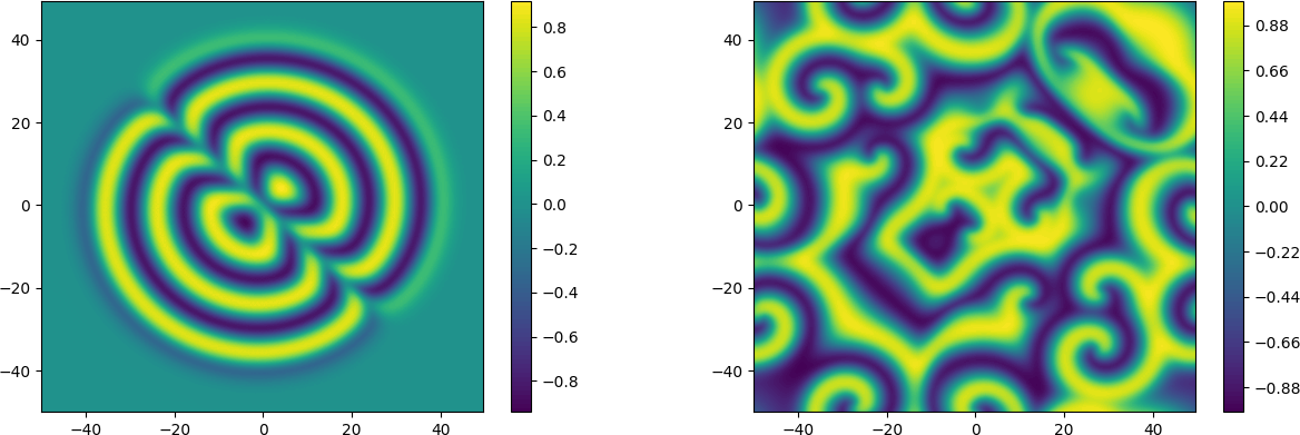
The code that is described here will run in parallel for up to a maximum of \( \text{min}(N[0], N[1]) \) processors. But, being a 2D problem, a single processor is sufficient to solve the problem in reasonable time. The real part of \( u(\boldsymbol{x}, t) \) is shown in Figure 2 for times \( t=16 \) and \( t=96 \), where the solution is initialized from (63). The results starting from the real initial condition in (64) is shown for the same times in Figure 3. There are apparently good agreements with figures published from using chebfun on www.chebfun.org/examples/pde/GinzburgLandau.html. In particular, the subfigures in Figure 2 are identical by the eye norm. One interesting feature, though, is seen in the right plot of Figure 3, where the results can be seen to have preserved symmetry, as they should. This symmetry is lost with chebfun, as commented in the referenced webpage. An asymmetric solution is also obtained with shenfun if no de-aliasing is applied. However, the simulations are very sensitive to roundoff, and it has also been observed that a de-aliased solution using shenfun may loose symmetry simply if a different FFT algorithm is chosen on runtime by FFTW.
Figure 2: Ginzburg-Landau solution (real) at times 16 and 96, from complex initial condition.
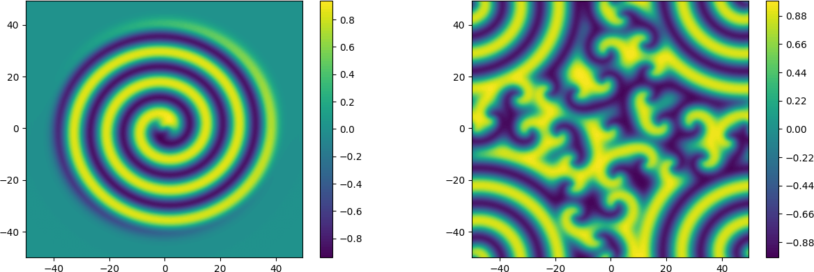
Figure 3: Ginzburg-Landau solution (real) at times 16 and 96 from real initial condition.