Shenfun
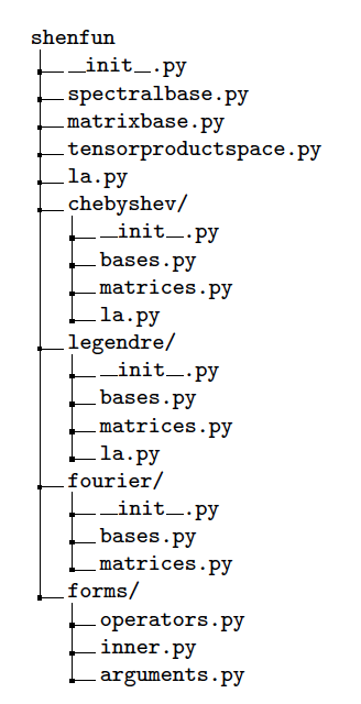
shenfun is a Python module package containing tools for working with the spectral Galerkin method. Shenfun implements classes for several bases with different boundary conditions, and within each class there are methods for transforms between spectral and real space, inner products, and for computing matrices arising from bilinear forms in the spectral Galerkin method. The Python module is organized as shown in Figure 1.
The shenfun language is very simple and closely follows that of FEniCS. A simple form implementation provides operators div, grad, curl and Dx, that act on three different types of basis functions, the TestFunction, TrialFunction and Function. Their usage is very similar to that from FEniCS, but not as general, nor flexible, since we are only conserned with simple tensor product grids and smooth solutions. The usage of these operators and basis functions will become clear in the following subchapters, where we will also describe the inner and project functions, with functionality as suggested by their names.
Figure 1: Directory tree.
Classes for basis functions
The following bases are defined in submodules
- shenfun.chebyshev.bases
- Basis - Regular Chebyshev
- ShenDirichletBasis - Dirichlet boundary conditions
- ShenNeumannBasis - Neumann boundary conditions (homogeneous)
- ShenBiharmonicBasis - Homogeneous Dirichlet and Neumann boundary conditions
- shenfun.legendre.bases
- Basis - Regular Legendre
- ShenDirichletBasis - Dirichlet boundary conditions
- ShenNeumannBasis - Neumann boundary conditions (homogeneous)
- ShenBiharmonicBasis - Homogeneous Dirichlet and Neumann boundary conditions
- shenfun.fourier.bases
- R2CBasis - Real to complex Fourier transforms
- C2CBasis - Complex to complex transforms
uc array is only used to test that the transform cycle returns the original data.
    >>> from shenfun import *
    >>> import numpy as np
    >>> N = 16
    >>> FFT = fourier.bases.R2CBasis(N)
    >>> u = np.random.random(N)
    >>> uc = u.copy()
    >>> u_hat = FFT.forward(u)
    >>> u = FFT.backward(u_hat)
    >>> assert np.allclose(u, uc)
Classes for matrices
Matrices that arise with the spectral Galerkin method using Fourier or Shen's modified basis functions (see, e.g., Eqs (23), (24)), are typically sparse and diagonal in structure. The sparse structure allows for a very compact storage, andshenfun has its own Matrix-class that is subclassing a Python dictionary, where keys are diagonal offsets, and values are the values along the diagonal. Some of the more important methods of the SparseMatrix class are shown below:
class SparseMatrix(dict):
    def __init__(self, d, shape):
        dict.__init__(self, d)
        self.shape = shape

    def diags(self, format='dia'):
        """Return Scipy sparse matrix"""

    def matvec(self, u, x, format='dia', axis=0):
        """Return Matrix vector product self*u in x"""

    def solve(self, b, u=None, axis=0):
        """Return solution u to self*u = b"""
For example, we may declare a tridiagonal matrix of shape N x N as
    >>> N = 4
    >>> d = {-1: 1, 0: -2, 1: 1}
    >>> A = SparseMatrix(d, (N, N))
or similarly as
    >>> d = {-1: np.ones(N-1), 0: -2*np.ones(N)}
    >>> d[1] = d[-1]  # Symmetric, reuse np.ones array
    >>> A = SparseMatrix(d, (N, N))
    >>> A
    {-1: array([ 1.,  1.,  1.]),
      0: array([-2., -2., -2., -2.]),
      1: array([ 1.,  1.,  1.])}
The matrix is a subclassed dictionary. If you want a regular Scipy sparse matrix instead, with all of its associated methods (solve, matrix-vector, etc.), then it is just a matter of
    >>> A.diags()
    <4x4 sparse matrix of type '<class 'numpy.float64'>'
        with 10 stored elements (3 diagonals) in DIAgonal format>
    >>> A.diags().toarray()
    array([[-2.,  1.,  0.,  0.],
           [ 1., -2.,  1.,  0.],
           [ 0.,  1., -2.,  1.],
           [ 0.,  0.,  1., -2.]])
Variational forms in 1D
Weak variational forms are created using test and trial functions, as shown in the section Spectral Galerkin Method. Test and trial functions can be created for any basis inshenfun, as shown below for a Chebyshev Dirichlet basis with 8 quadrature points
    >>> from shenfun.chebyshev.bases import ShenDirichletBasis
    >>> from shenfun import inner, TestFunction, TrialFunction
    >>> N = 8
    >>> SD = ShenDirichletBasis(N)
    >>> u = TrialFunction(SD)
    >>> v = TestFunction(SD)
A bilinear form contains both test- and trialfunctions, whereas a linear form contains only the testfunction. Assembling a biliear form results in a matrix, whereas assembling a linear form results in a vector.
A matrix that is the result of a bilinear form has its own subclass of SparseMatrix, called a SpectralMatrix. A SpectralMatrix is created using inner products on test and trial functions, for example the mass matrix:
    >>> mass = inner(u, v)
    >>> mass
    {-2: array([-1.57079633]),
      0: array([ 4.71238898,  3.1415
                 3.14159265, 3.14159265]),
      2: array([-1.57079633])}
This mass matrix will be the same as Eq. (2.5) of [1], and it will be an instance of the SpectralMatrix class.
You may notice that mass takes advantage of the fact that two diagonals are constant and consequently only stores one single value.
The inner method may be used to compute any linear or bilinear form. For
example, the stiffness matrix K may be computed with the bilinear form
>>> K = inner(v, div(grad(u)))
Square matrices have implemented a solve method that is using fast
\( \mathcal{O}(N) \) direct LU decomposition or similar, if available, and falls
back on using Scipy's solver in CSR format if no better method is found
implemented. For example, to solve the linear system Ku_hat=b_hat
    >>> fj = np.random.random(N)
    >>> b_hat = inner(v, fj)
    >>> u_hat = np.zeros_like(b_hat)
    >>> u_hat = K.solve(b_hat, u_hat)
Most methods are designed to work along any dimension of a multidimensional array. Very little differs in the users interface. Consider, for example, the previous example on a three-dimensional cube
    >>> f3 = fj.repeat(N**2).reshape((N, N, N)) # Array f3 of shape (N,N,N)
    >>> u3 = np.zeros_like(f3)
    >>> u3 = K.solve(f3, u3)
where K is exactly the same as before, from the 1D example. The matrix solve is applied along the first dimension since this is the default behaviour.
The bases also have methods for transforming between spectral and real space. For example, one may project a random vector to the SD space using
    >>> fj = np.random.random(N)
    >>> fk = np.zeros_like(fj)
    >>> fk = SD.forward(fj, fk) # Gets expansion coefficients
and back to real physical space again
>>> fj = SD.backward(fk, fj)
Note that fj now will be different than the original fj since it now has homogeneous boundary conditions. However, if we transfer back and forth one more time, starting from fj which is in the Dirichlet function space, then we come back to the same array:
    >>> fj_copy = fj.copy()
    >>> fk = SD.forward(fj, fk)
    >>> fj = SD.backward(fk, fj)
    >>> assert np.allclose(fj, fj_copy) # Is True
Poisson equation implemented in 1D
We have now shown the usage of shenfun for single, one-dimensional spaces. It does not become really interesting before we start looking into tensor product grids in higher dimensions, but before we go there we revisit the spectral Galerkin method for a 1D Poisson problem, and show how the implementation of this problem can be performed using shenfun.
Periodic boundary conditions
If the solution to Eq. (1) is periodic with periodic length \( 2 \pi \), then we use \( \Omega \in [0, 2 \pi] \) and it will be natural to choose the test functions from the space consisting of the Fourier basis functions, i.e., \( v_l(x)=e^{ilx} \). The mesh \( \boldsymbol{x} = \{x_j\}_{j=0}^{N-1} \) will be uniformly spaced $$ \begin{equation} \boldsymbol{x} = \frac{2 \pi j}{N} \quad j=0,1,\ldots, N-1, \tag{6} \end{equation} $$ and we look for solutions of the form $$ \begin{equation} u(x_j) = \sum_{l=-N/2}^{N/2-1} \hat{u}_l e^{ilx_j} \quad j=0,1,\ldots N-1. \tag{7} \end{equation} $$ Note that for Fourier basis functions it is customary (used by both MATLAB and Numpy) to use the wavenumbermesh $$ \begin{equation} \boldsymbol{l} = -N/2, -N/2+1, \ldots, N/2-1, \tag{8} \end{equation} $$ where we have assumed that \( N \) is even. Also note that Eq. (7) naively would be computed in \( \mathcal{O}(N^2) \) operations, but that it can be computed much faster \( \mathcal{O}(N\log N) \) using the discrete inverse Fourier transform $$ \begin{equation} \bs{u} = \mathcal{F}^{-1}(\bs{\hat{u}}), \tag{9} \end{equation} $$ where we use compact notation \( \bs{u} = \{u(x_j)\}_{j=0}^{N-1} \).To solve Eq. (1) with the discrete spectral Galerkin method, we create the basis \( V^p = \text{span}\{ e^{ilx} , \text{ for } l \in \boldsymbol{l}\} \) and attempt to find \( u \in V^p \) such that $$ \begin{equation} (-u'', v)_w^N = (f, v)_w^N, \quad \forall \, v \in V^p. \tag{10} \end{equation} $$ Inserting for Eq. (7) and using \( e^{imx} \) as test function we obtain $$ \begin{align} -(\sum_{l \in \bs{l}} \hat{u}_l (e^{ilx})'', e^{imx})_w^N &= (f(x), e^{imx})_w^N \quad \forall \, m \in \bs{l} \tag{11}\\ \sum_{l \in \bs{l}} l^2( e^{ilx}, e^{imx})_w^N \hat{u}_l &= (f(x), e^{imx})_w ^N\quad \forall \, m \in \bs{l}. \tag{12} \end{align} $$ Note that the discrete inner product (5) is used, and we also need to interpolate the function \( f(x) \) onto the grid \( \boldsymbol{x} \). For Fourier it becomes very simple since the weight functions are constant \( w_j = 2\pi/N \) and we have for the left hand side simply a diagonal matrix $$ \begin{equation} ( e^{ilx}, e^{imx})^N = 2\pi \delta_{ml} \quad \text{for} \, l, m \in \bs{l} \times \bs{l}, \tag{13} \end{equation} $$ where \( \delta_{ml} \) is the kronecker delta function. For the right hand side we have $$ \begin{align} (f(x), e^{imx})^N &= \frac{2 \pi}{N}\sum_{j=0}^{N-1} f(x_j) e^{-imx_j} \quad \text{for } m \in \bs{l}, \tag{14}\\ &= 2 \pi \mathcal{F}_m(f(\bs{x})), \tag{15}\\ &= 2 \pi \hat{f}_m, \tag{16} \end{align} $$ where \( \mathcal{F} \) represents the discrete Fourier transform that is defined as $$ \begin{equation} \hat{u}_l = \frac{1}{N}\sum_{j=0}^{N-1} u(x_j) e^{-ilx_j}, \quad \text{for } l \in \bs{l}, \tag{17} \end{equation} $$ or simply $$ \begin{equation} \bs{\hat{u}} = \mathcal{F}(\bs{u}). \tag{18} \end{equation} $$ Putting it all together we can set up the assembled linear system of equations for \( \hat{u}_l \) in (12) $$ \begin{equation} \sum_{l \in \bs{l}}2 \pi l^2 \delta_{ml} \hat{u}_l = 2 \pi \hat{f}_{m} \quad \forall \, m \in \bs{l}, \tag{19} \end{equation} $$ which is trivially solved since it only involves a diagonal matrix (\( \delta_{ml} \)), and we obtain $$ \begin{equation} \hat{u}_l = \frac{1}{l^2} \hat{f}_{l} \quad \forall \,l \in \bs{l} \setminus{\{0\}}. \tag{20} \end{equation} $$
So, even though we carefully followed the spectral Galerkin method, we have ended up with the same result that would have been obtained with a Fourier collocation method, where one simply takes the Fourier transform of the Poisson equation and differentiate analytically.
With shenfun the periodic 1D Poisson equation can be trivially computed either with the collocation approach or the spectral Galerkin method. The procedure for the spectral Galerkin method will be shown first, before the entire problem is solved. All shenfun demos in this paper will contain a similar preample section where some necessary Python classes, modules and functions are imported. We import Numpy since shenfun arrays are Numpy arrays, and we import from Sympy to construct some exact solution used to verify the code. Note also the similarity to FEniCS with the import of methods and classes inner, div, grad, TestFunction, TrialFunction. The Fourier spectral Galerkin method in turn requires that the FourierBasis is imported as well. The following code solves the Poisson equation in 1D with shenfun:
from sympy import Symbol, cos
import numpy as np
from shenfun import inner, div, grad, TestFunction, TrialFunction
from shenfun.fourier.bases import FourierBasis

# Use Sympy to compute a rhs, given an analytical solution
x = Symbol("x")
ue = cos(4*x)
fe = ue.diff(x, 2)

# Create Fourier basis with N basis functions
N = 32
ST = FourierBasis(N, np.float)
u = TrialFunction(ST)
v = TestFunction(ST)
X = ST.mesh(N)

# Get f and exact solution on quad points
fj = np.array([fe.subs(x, j) for j in X], dtype=np.float)
uj = np.array([ue.subs(x, i) for i in X], dtype=np.float)

# Assemble right and left hand sides
f_hat = inner(v, fj)
A = inner(v, div(grad(u)))

# Solve Poisson equation
u_hat = A.solve(f_hat)

# Transfer solution back to real space
uq = ST.backward(u_hat)
assert np.allclose(uj, uq)
Naturally, this simple problem could be solved easier with a Fourier collocation instead, and a simple pure 1D Fourier problem does not illuminate the true advantages of shenfun, that only will become evident when we look at higher dimensional problems with tensor product spaces. To solve with collocation, we could simply do
# Transform right hand side
f_hat = ST.forward(fj)

# Wavenumers
k = ST.wavenumbers(N)
k[0] = 1

# Solve Poisson equation (solution in f_hat)
f_hat /= k**2

# Transform to real space
uq = ST.backward(f_hat)
Note that ST methods forward/backward correspond to forward and inverse discrete Fourier transforms. Furthermore, since the input data fj is of type float (not complex), the transforms make use of the symmetry of the Fourier transform of real data, that \( \hat{u}_k = \overline{\hat{u}}_{N-k} \), and that \( \bs{k}=0,1,\ldots, N/2 \) (index set computed as k = ST.wavenumbers(N)).
Dirichlet boundary conditions
If the Poisson equation is subject to Dirichlet boundary conditions on the edge of the domain \( \Omega \in [-1, 1] \), then a natural choice is to use Chebyshev or Legendre polynomials. Two test functions that strongly fixes the boundary condition \( u(\pm 1)=0 \) are $$ \begin{equation} v_l(x) = T_l(x) - T_{l+2}(x), \tag{21} \end{equation} $$ where \( T_l(x) \) is the l'th order Chebyshev polynomial of the first kind, or $$ \begin{equation} v_l(x) = L_l(x) - L_{l+2}(x), \tag{22} \end{equation} $$ where \( L_l(x) \) is the l'th order Legendre polynomial. The test functions give rise to functionspaces $$ \begin{align} V^C &= \text{span}\{T_l-T_{l+2}, l \in \bs{l}^D\}, \tag{23} \\ V^L &= \text{span}\{L_l-L_{l+2}, l \in \bs{l}^D\}, \tag{24} \end{align} $$ where $$ \begin{equation} \boldsymbol{l}^D = 0, 1, \ldots, N-3. \tag{25} \end{equation} $$ The computational mesh and associated weights will be decided by the chosen quadrature rule. Here we will go for Gauss quadrature, which leads to the following points and weights for the Chebyshev basis $$ \begin{align} x_j^C &= \cos \left( \frac{2j+1}{2N}\pi \right) \quad &j=0,1,\ldots, N-1, \tag{26}\\ w_j^C &= \frac{\pi}{N}, \tag{27} \end{align} $$ and $$ \begin{align} x_j^L &= \text{ zeros of }L_{N}(x) \quad &j=0,1,\ldots, N-1, \tag{28}\\ w_j^L &= \frac{2}{(1-x_j^2)[L'_{N}(x_j)]^2} \quad &j=0,1,\ldots, N-1, \tag{29} \end{align} $$ for the Legendre basis.We now follow the same procedure as in the section Periodic boundary conditions and solve Eq. (1) with the spectral Galerkin method. Consider first the Chebyshev basis and find \( u \in V^C \) , such that $$ \begin{equation} (-u'', v)_w^N = (f, v)_w^N , \quad \forall \, v \in V^C. \tag{30} \end{equation} $$ We insert for \( v=v_m \) and \( u=\displaystyle \sum_{l\in \bs{l}^D} \hat{u}_l v_l \) and obtain $$ \begin{align} -(\sum_{l\in \bs{l}^D} \hat{u}_l v_l'', v_m)_w^N &= (f, v_m)_w^N &m \in \bs{l}^D, \tag{31}\\ -(v_l'', v_m)_w^N \hat{u}_l &= (f, v_m)_w^N & m \in \bs{l}^D, \tag{32} \end{align} $$ where summation on repeated indices is implied. In Eq. (32) \( A_{ml} =(v_l'', v_m)_w^N \) are the components of a sparse stiffness matrix, and we will use matrix notation \( \bs{A} = \{A_{ml}\}_{m,l \in \bs{l}^D \times \bs{l}^D} \) to simplify. The right hand side can similarily be assembled to a vector with components \( \tilde{f}_m = (f, v_m)_w^N \) such that \( \bs{\tilde{f}} = \{\tilde{f}_m\}_{m\in \bs{l}^D} \). Note that a tilde is used since this is not a complete transform. We can now solve for the unknown \( \bs{\hat{u}} = \{\hat{u}_l\}_{l\in \bs{l}^D} \) vector $$ \begin{align} -\bs{A} \bs{\hat{u}} &= \bs{\tilde{f}}, \tag{33}\\ \bs{\hat{u}} &= -\bs{A}^{-1} \bs{\tilde{f}}. \tag{34} \end{align} $$ Note that the matrix \( \bs{A} \) is a special kind of upper triangular matrix, and that the solution can be obtained very efficiently in approximately \( 4 N \) arithmetic operations.
To get the solution back and forth between real and spectral space we require a transformation pair similar to the Fourier transforms. We do this by projection. Start with $$ \begin{equation} u(\bs{x}) = \sum_{l\in \bs{l}^D} \hat{u}_l v_l(\bs{x}) \tag{35} \end{equation} $$ and take the inner product with \( v_m \) $$ \begin{equation} (u, v_m)_w^N = (\sum_{l\in \bs{l}^D} \hat{u}_l v_l, v_m)_w^N. \tag{36} \end{equation} $$ Introducing now the mass matrix \( B_{ml} = (v_l, v_m)_w^N \) and the Shen forward inner product \( \mathcal{S}_m(u) = (u, v_m)_w^N \), Eq. (36) is rewritten as $$ \begin{align} \mathcal{S}_m(u) &= B_{ml} \hat{u}_l, \tag{37}\\ \bs{\hat{u}} =& \bs{B}^{-1} \mathcal{S}(\bs{u}) , \tag{38}\\ \bs{\hat{u}} =& \mathcal{T}(\bs{u}) , \tag{39} \end{align} $$ where \( \mathcal{T}(\bs{u}) \) represents a forward transform of \( \bs{u} \). Note that \( \mathcal{S} \) is introduced since the inner product \( (u, v_m)_w^N \) may, just like the inner product with the Fourier basis, be computed fast, with \( \mathcal{O}(N \log N) \) operations. And to this end, we need to make use of a discrete cosine transform (DCT), instead of the Fourier transform. The details are left out from this paper, though.
A simple Poisson problem with analytical solution \( \sin(\pi x)(1-x^2) \) is implemented below, where we also verify that the correct solution is obtained.
from sympy import Symbol, sin, lambdify
import numpy as np
from shenfun import inner, div, grad, TestFunction, TrialFunction
from shenfun.chebyshev.bases import ShenDirichletBasis

# Use sympy to compute a rhs, given an analytical solution
x = Symbol("x")
ue = sin(np.pi*x)*(1-x**2)
fe = ue.diff(x, 2)

# Lambdify for faster evaluation
ul = lambdify(x, ue, 'numpy')
fl = lambdify(x, fe, 'numpy')

N = 32
SD = ShenDirichletBasis(N)
X = SD.mesh(N)
u = TrialFunction(SD)
v = TestFunction(SD)
fj = fl(X)

# Compute right hand side of Poisson equation
f_hat = inner(v, fj)

# Get left hand side of Poisson equation and solve
A = inner(v, div(grad(u)))
f_hat = A.solve(f_hat)
uj = SD.backward(f_hat)

# Compare with analytical solution
ue = ul(X)
assert np.allclose(uj, ue)
Note that the inner product f_hat = inner(v, fj) is computed under the hood using the fast DCT. The inverse transform uj = SD.backward(f_hat) is also computed using a fast DCT, and we use the notation
$$
\begin{align}
u(x_j) &= \sum_{l\in \bs{l}^D} \hat{u}_l v_l(x_j) \quad j=0,1,\ldots, N-1, \notag
\tag{40}\\
\bs{u} &= \mathcal{S}^{-1}(\bs{\hat{u}}). \tag{41}
\end{align}
$$
To implement the same problem with the Legendre basis (22), all that is needed to change is the first line in the Poisson solver to from shenfun.legendre.bases import ShenDirichletBasis. Everything else is exactly the same. However, a fast inner product, like in (41), is only implemented for the Chebyshev basis, since there are no known \( \mathcal{O}(N \log N) \) algorithms for the Legendre basis, and the Legendre basis thus uses straight forward \( \mathcal{O}(N^2) \) algorithms for its transforms.