Lab 3: Memory Span Experiment and Statistics Review
Memory Span Experiment

Experimental Design Lingo
In general, an experiment is a procedure that researchers use to assess the effect of one variable (IV) on another variable (DV).
Independent variable (IV): In experiments, this is the variable that the researchers manipulate (e.g., randomly assigning participants to 2 different groups).
synonyms: Predictor variable, Explanatory variable.
Dependent variable (DV): In experiments, this is the variable of interest. This variable is expected to change according to the IV.
synonyms: Outcome variable, Response variable.
Control group or control condition: Baseline group. All other experimental groups are usually compared to this group.
synonyms: Comparison group, Placebo condition.
Variable types:
Continuous variables: Essentially numbers (e.g., 5.4).
Discrete variables: Gender, experimental condition (e.g., control VS treatment), Hair color, etc…
Ordinal variables will not come up in this lab
Experiment Instructions
Log into your CogLab account and click on “complete lab”
↓
Then, select “24.Memory Span”
↓
Please, Do not read the “background” or the “instructions”. Click here for the experiment instructions
↓
After you are done, you are free to scroll to the top and read the “background” section

About Memory Span
The term Memory span refers to the number of things one can remember after being shown a list of objects. On average, people can remember \(7\pm 2\) items.
What impacts memory span?
Type of items: A list of similar items (all numbers) is easier to remember than a list of unrelated items (some numbers, some colors, etc…)

Phonological Similarity: Memory span is lower when items in a sequence sound similar to other items in the sequence. For example, it is easier to correctly recall K R X L Y F than C P D V G T.

Item length: people can remember about as many words as they can say in two seconds (Baddeley, Thomson, & Buchanan, 1975). So, lists with shorter words are easier to remember than lists with longer words.
Statistics Review

Mean and Standard Deviation
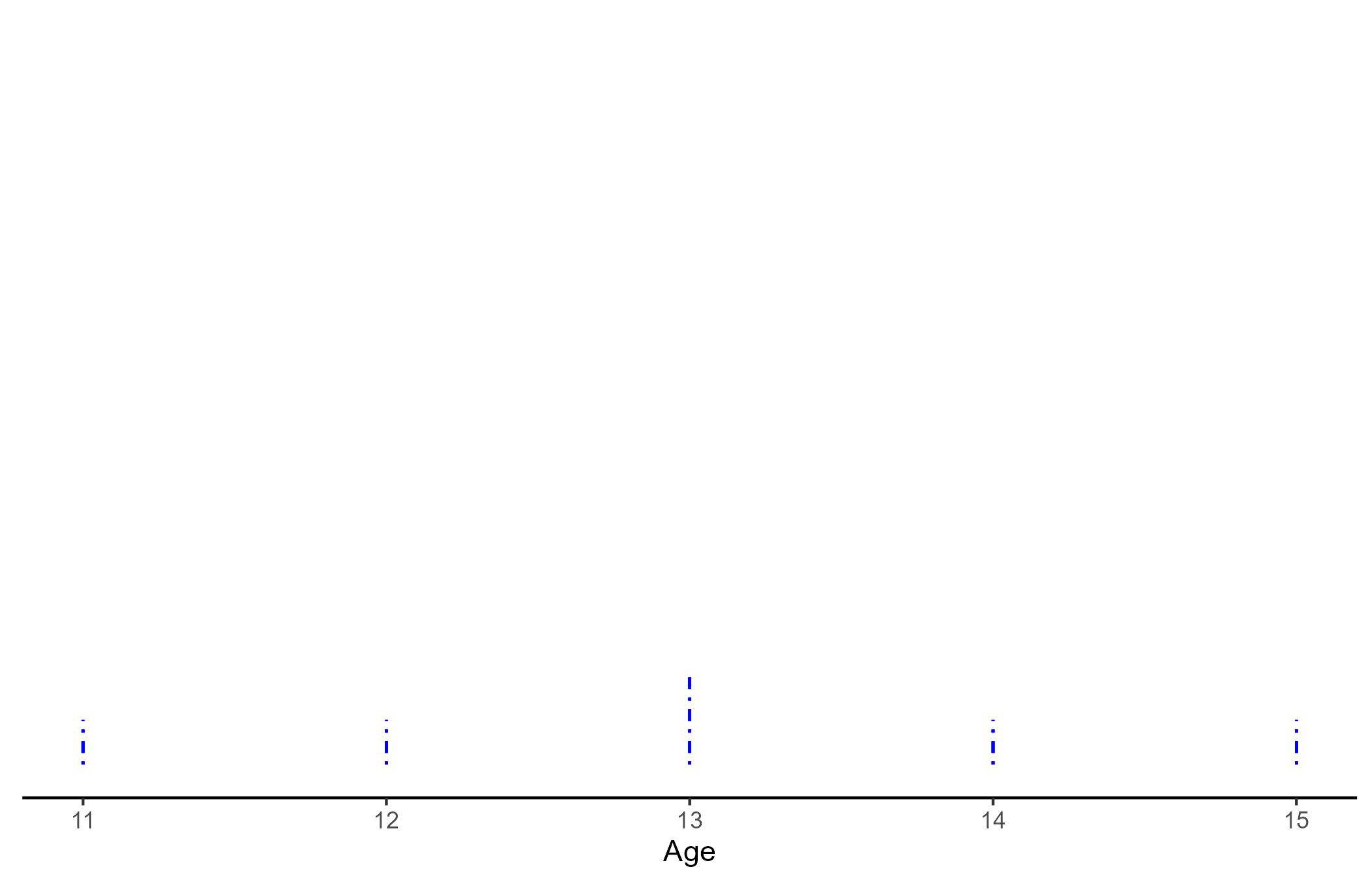
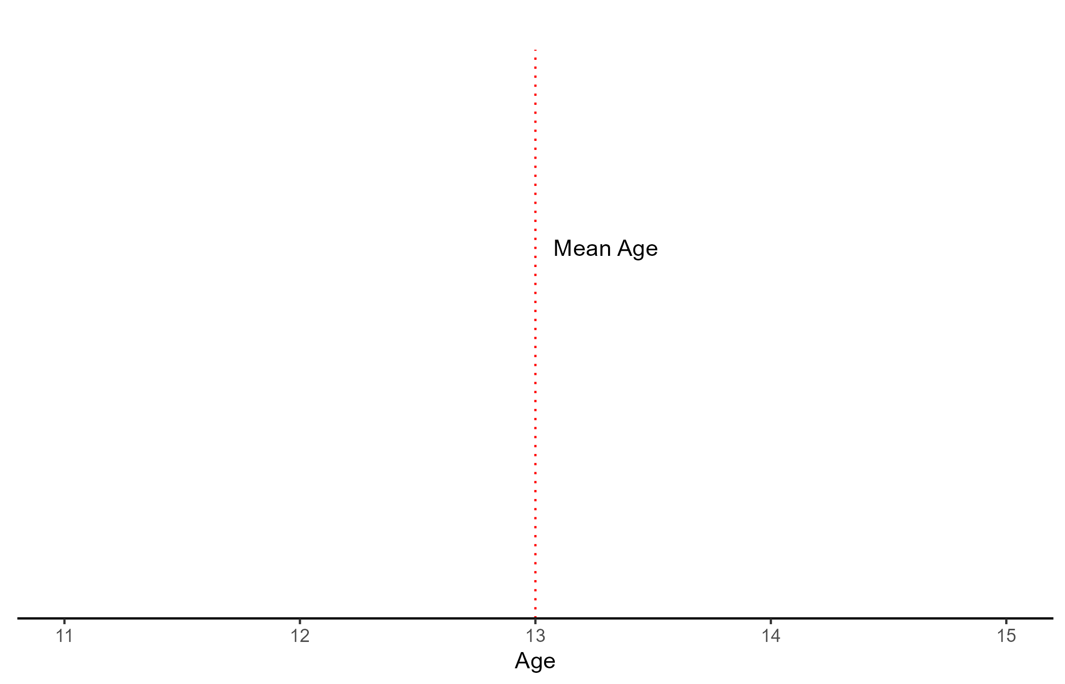
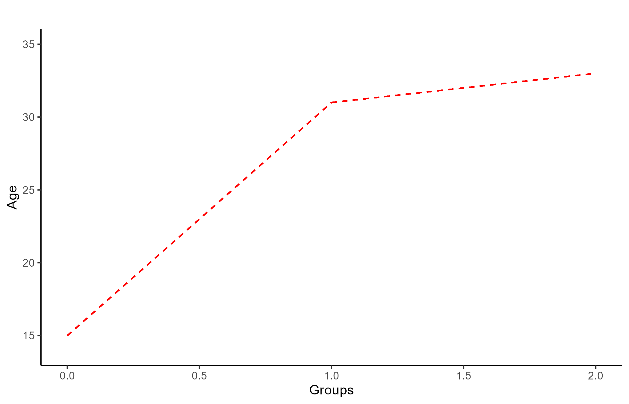
Although basic, the mean and standard deviation (SD) are very important concepts. Let us assume that we recorded the age of 6 people:
AGE
11, 12, 13, 13, 14 ,15
- \(Mean_{Age} = \frac{\sum Age_i}{N_{Age}} = \frac{11 + 12 + 13 + 13 +14 +15}{6} = 13\)
- \(SD_{Age} = \frac{\sqrt{\sum(Mean_{Age} - Age_i)^2}}{N_{Age}- 1} = 1.41\)
- \(SE_{Age} = \frac{SD_{Age}}{\sqrt{N_{Age}}} = 0.58\)
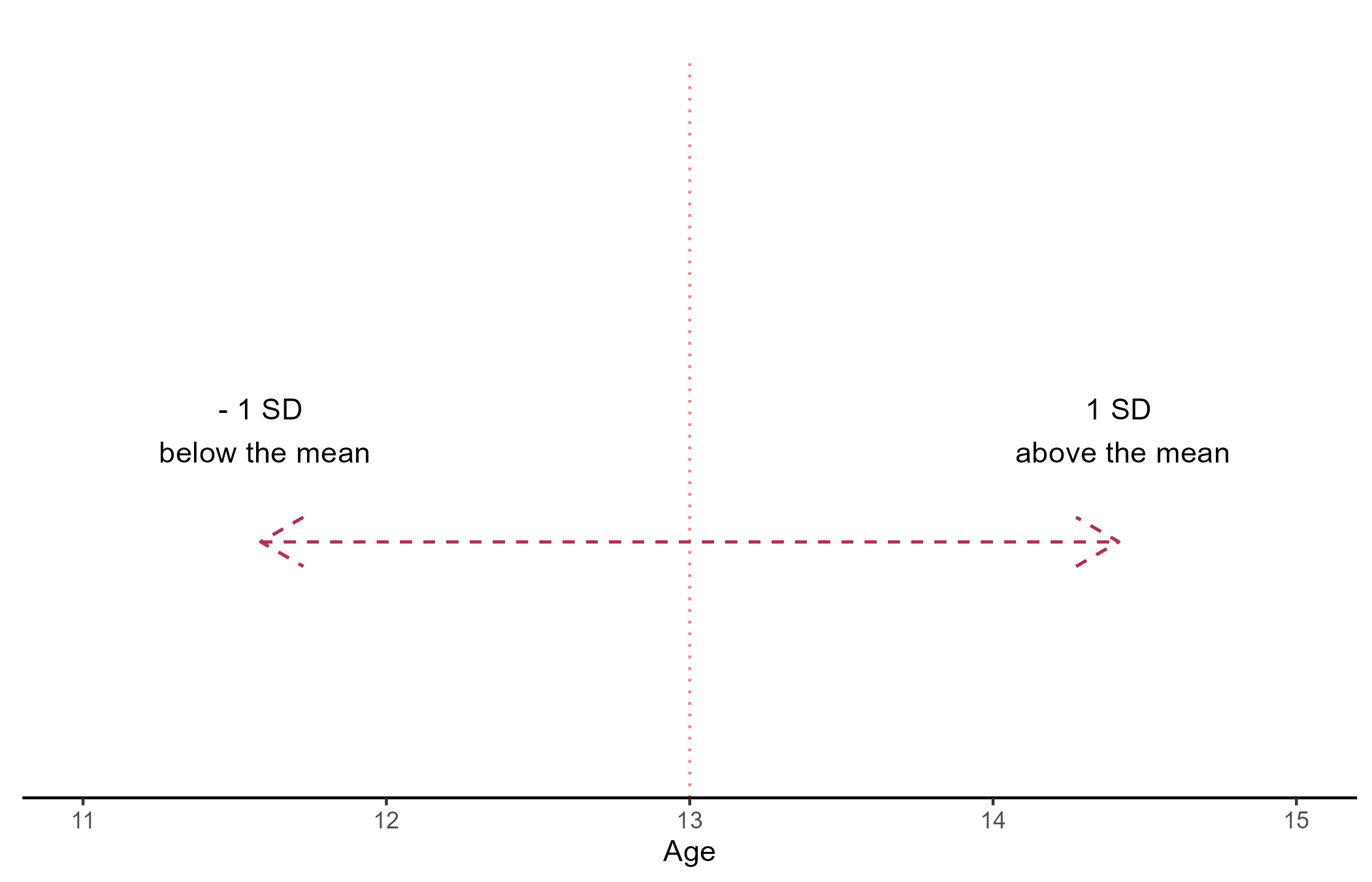
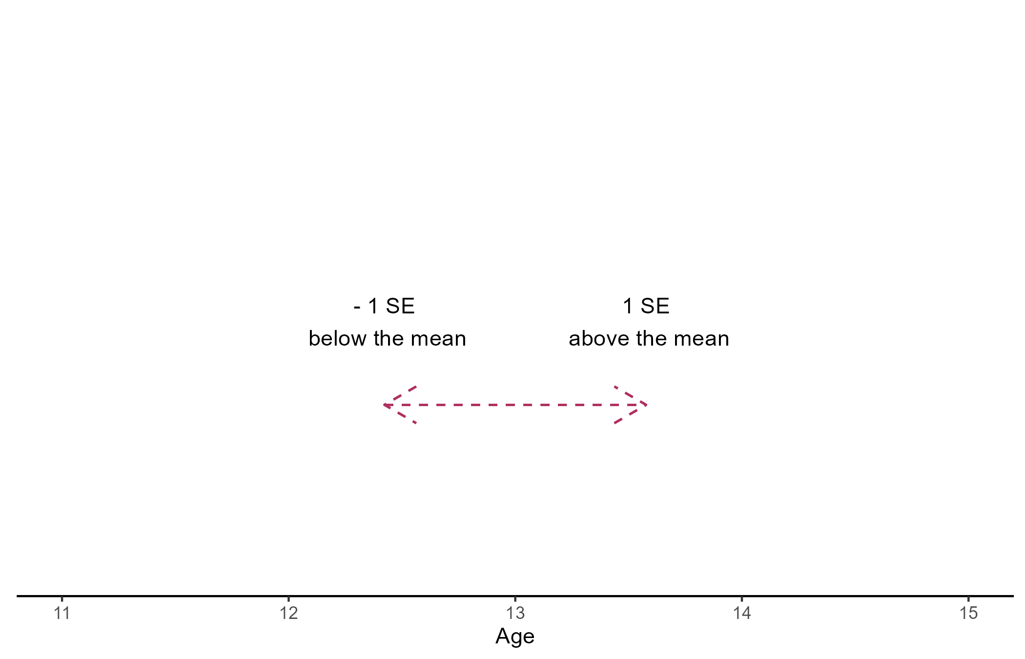
The mean is a measure of central tendency, and the standard deviation (SD) measures how spread out the data is. The standard error (SE) can be interpreted as the degree of confidence one can have that the sample mean is close to the true population mean (lower SE implies higher confidence).
Correlation and Regression
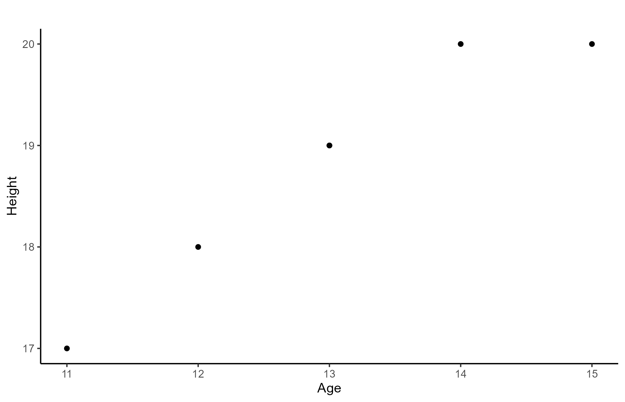
It turns out that one cannot calculate many statistics with just one variable 🤷 Let’s also assume that, aside from people’s age, we also measured their height:
Age: 11, 12, 13, 13, 14 ,15
Height: 17, 18, 19, 19, 20, 20
Astute observers 🧐 will probably notice a “tiny” upward trend. The Age and Height variables are indeed highly positively correlated, meaning that as age increases, so does height.
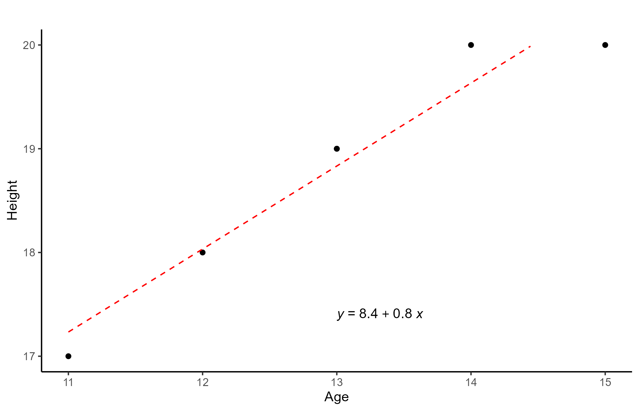
Regression simply plots the line that is closest to all the points. In our case, the line can be defined as \(Height_i = a + b\times Age_i\), were \(a\) represents where the line hits the Y-axis (y intercept) and \(b\) is the line slope.


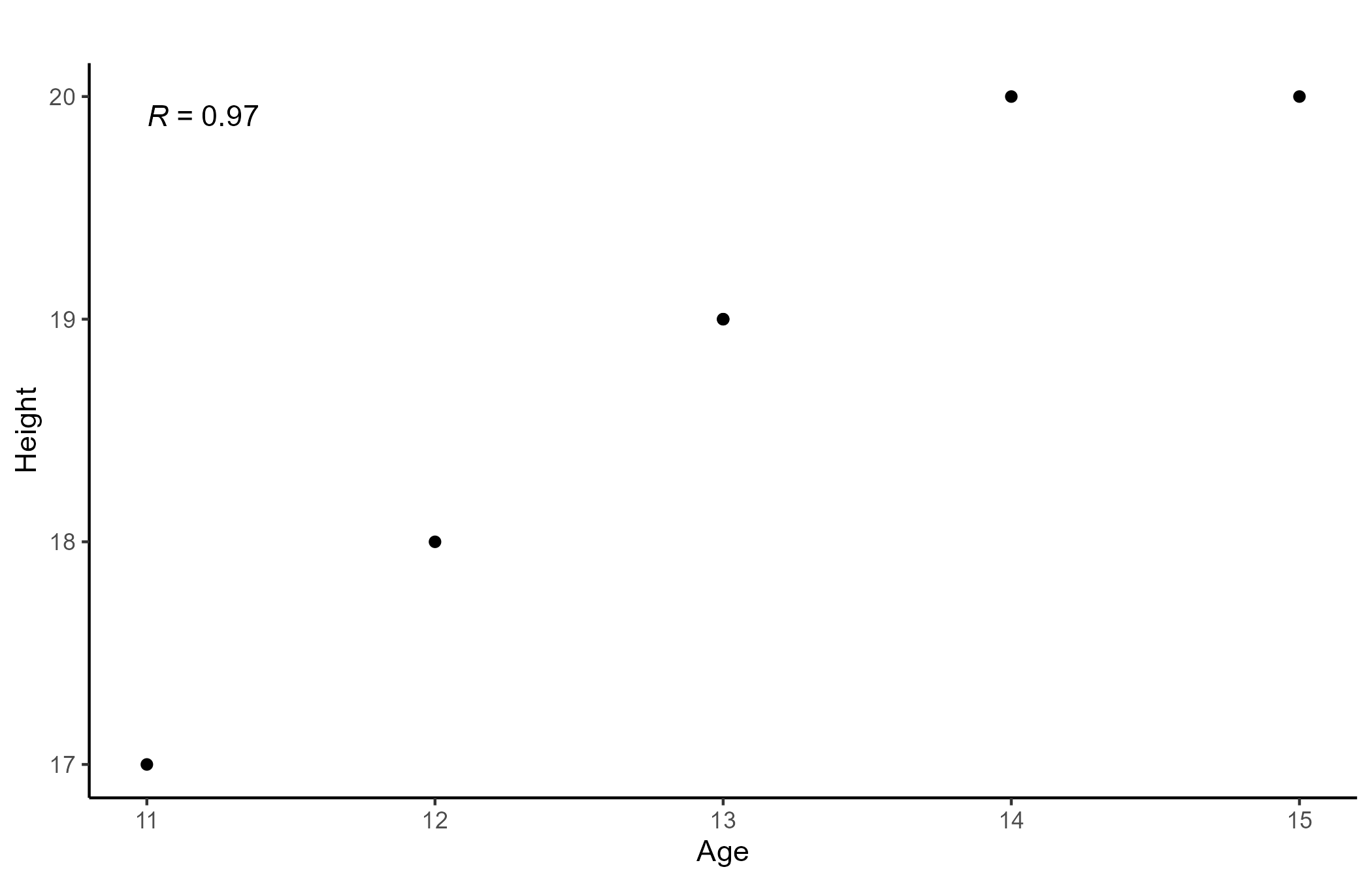
NOTE: Correlation and regression carry very similar information. For instance, the correlation coefficient and the line slope are equivalent, \(R = b\times \frac{SD_{Age}}{SD_{Height}} = 0.8 \times \frac{1.4}{1.17} \approx .97\)
T-tests
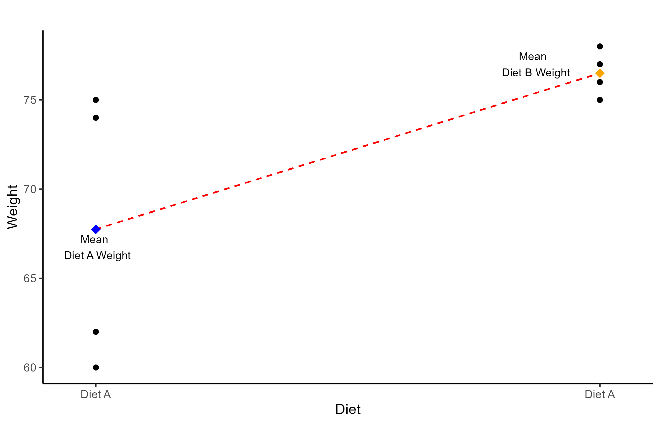
Personally, I think that t-tests are often taught in a way that causes some confusion. Normally, we teach that one should run a t-test when we want to compare the means of 2 groups. That is true, but slightly misleading.
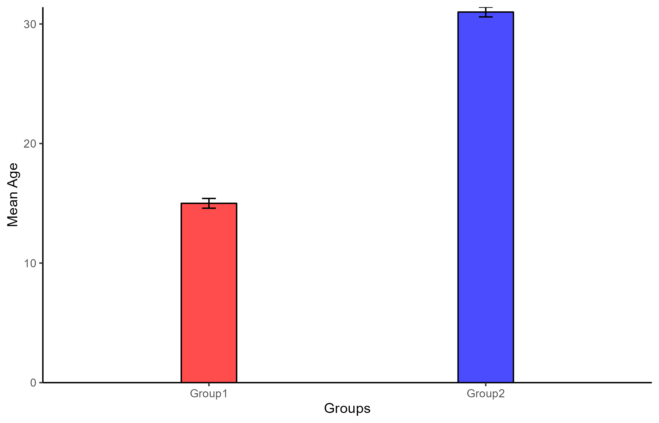
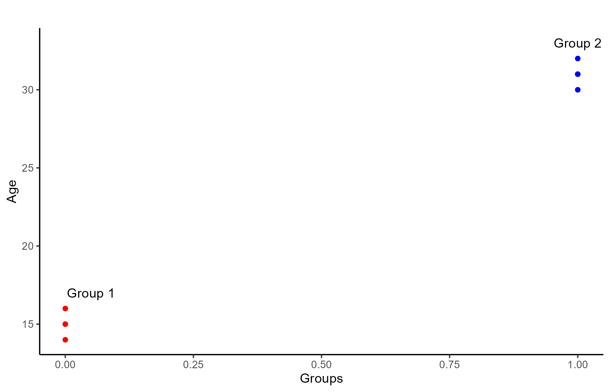
Let us assume that we measured the age of two groups of people (Group 1, group 2)
AGE
14, 15, 15, 16, 30, 31, 31, 32
if we input the values above in our trusty t-test calculator, we will find that the two group means are highly significantly different, \(\Delta M\) = 16, t(6) = 27.71, p < .001.
In other words, we are extremely confident that the 16 mean difference in Age between the two groups did not happen by chance (i.e., it is significantly different from 0) .
And this is your vanilla t-test, but there is more that statisticians don’t want you to know…😶

T-test but it’s Actually a Regression 🤯
Bar plots are one of the most common ways of displaying mean differences between groups, you can also use scatter plots by assigning each group a number (usually 0 and 1).
Although this is a bit of a strange looking scatter plot, you can still draw a regression line through the points!
The slope of the regression line is 16, which is exactly the mean difference between the two groups! Additionally, the intercept of the line is exactly the mean of Group 1 (labeled as “0”).
The results that appear in t-tests come from testing whether the regression slope is significantly different from 0. In papers, you would see this reported as b = 16, t(6) = 27.71, p < .001 (the exact same result of the t-test on the previous slide!).
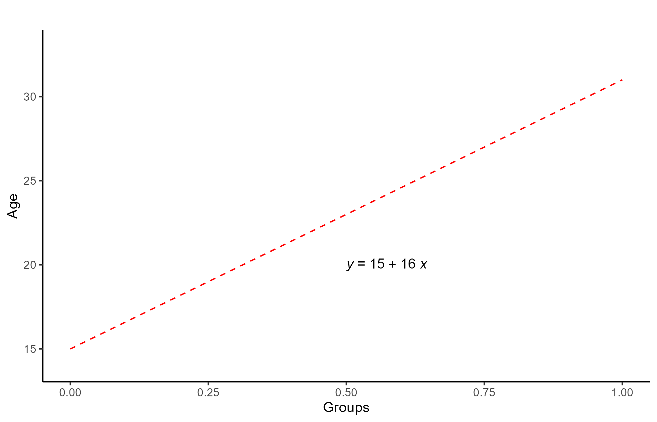
In other words, There is no difference between a t-test and a regression.
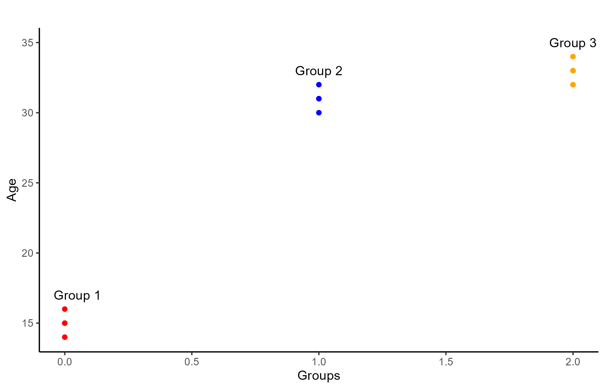
One-Way ANOVAs
Although scary sounding, a one-way ANOVA is simply a direct extension of t-test! The only difference is that it deals with the case in which there are more than 2 groups.
AGE
14, 15, 15, 16, 30, 31, 31, 32, 32, 33, 33, 34
Once again, one-way ANOVA is also a glorified regression, and the visualization is very similar to that of a t-test. The equivalence to regression takes a bit longer to show, so I will omit it for the sake of time.
The main difference with t-tests is that one-way ANOVAs produces an F statistics instead of a t statistic. If we input the data in a one-way ANOVA calculator, the result is F(2,9) = 583.99, p <.001.
The interpretation of a significant one-way ANOVA is that we are confident that the mean of the DV (Age here) changes depending on the IV (Group here). If one so wishes, it is also possible to run multiple t-tests to see which two group means are significantly different from each other (known as post hoc, or pairwise comparison).
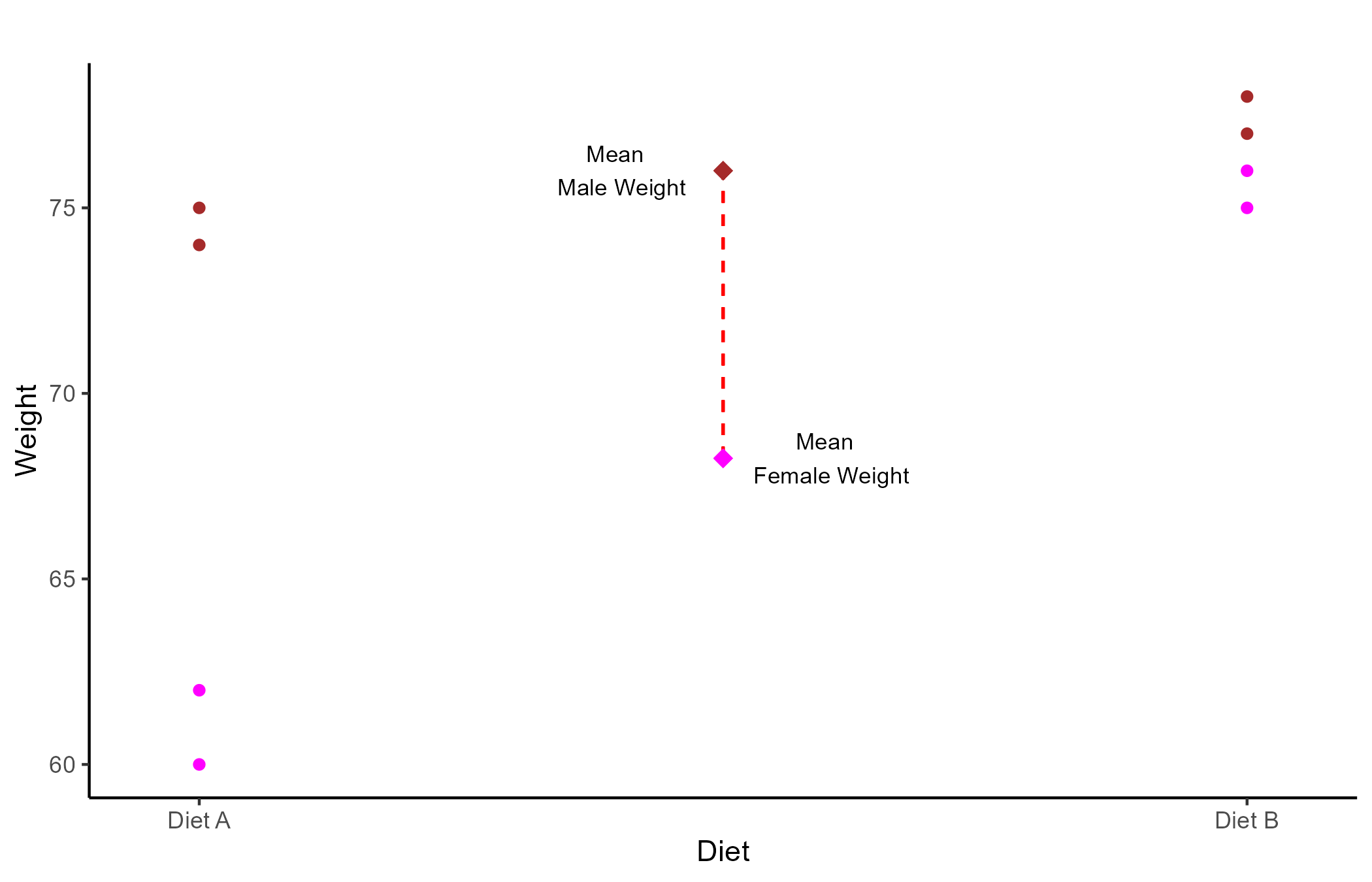
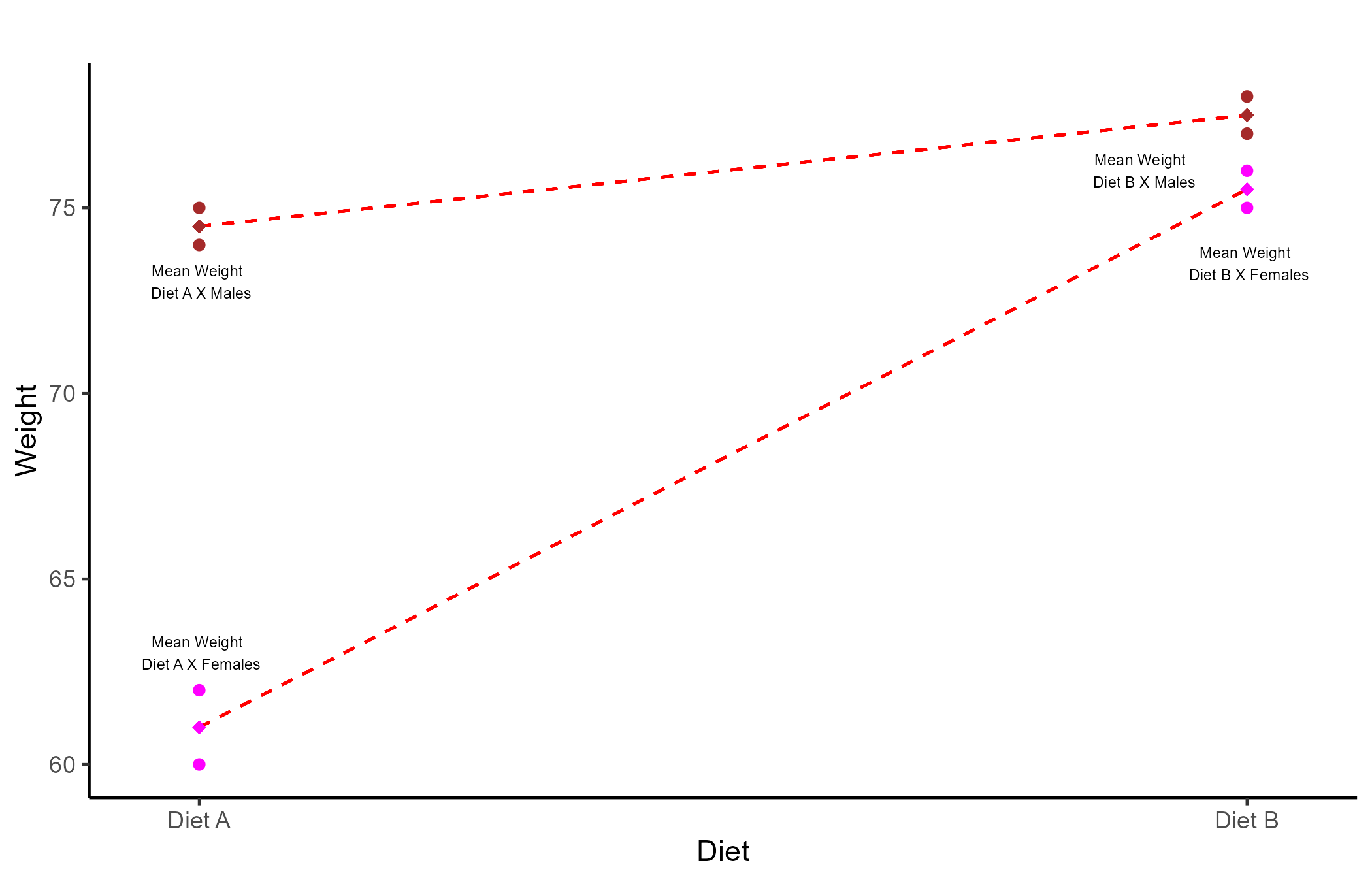
Two-Way ANOVAs
Finally, a two-way ANOVA (yes, also a regression) is generally used when there are 2 categorical IVs (usually two grouping variables).
Let’s say that we randomly sample 4 males and 4 females all weighting 80 kilos. Further, we assign diet A to 2 random male/females and diet B to the remaining people. After 3 months we measure the weight of all the participants:
| Diet A | Diet B | |
|---|---|---|
| Female | 60, 62 | 75, 76 |
| Male | 74, 75 | 74, 77 |
the two-way ANOVA calculator gives the 3 following results:
- Main effect of Diet: Weight after 3 months changes significantly depending on the type of diet that participants are assigned to, F(1, 4) = 64.07, p=.001.
- Main effect of Gender: Weight after 3 months changes significantly depending on gender, F(1, 4) = 48.6, p = .002.
- Interaction effect of Gender\(\times\)Diet: The effect of the type of diet on weight after 3 months, changes significantly depending on what gender participants are, F(1, 4) = 48.6, p = .002.
The results that Two-way ANOVA provides are the two main effects of the IVs, which are the same as running two separate one-way ANOVAs, and an interaction effect.
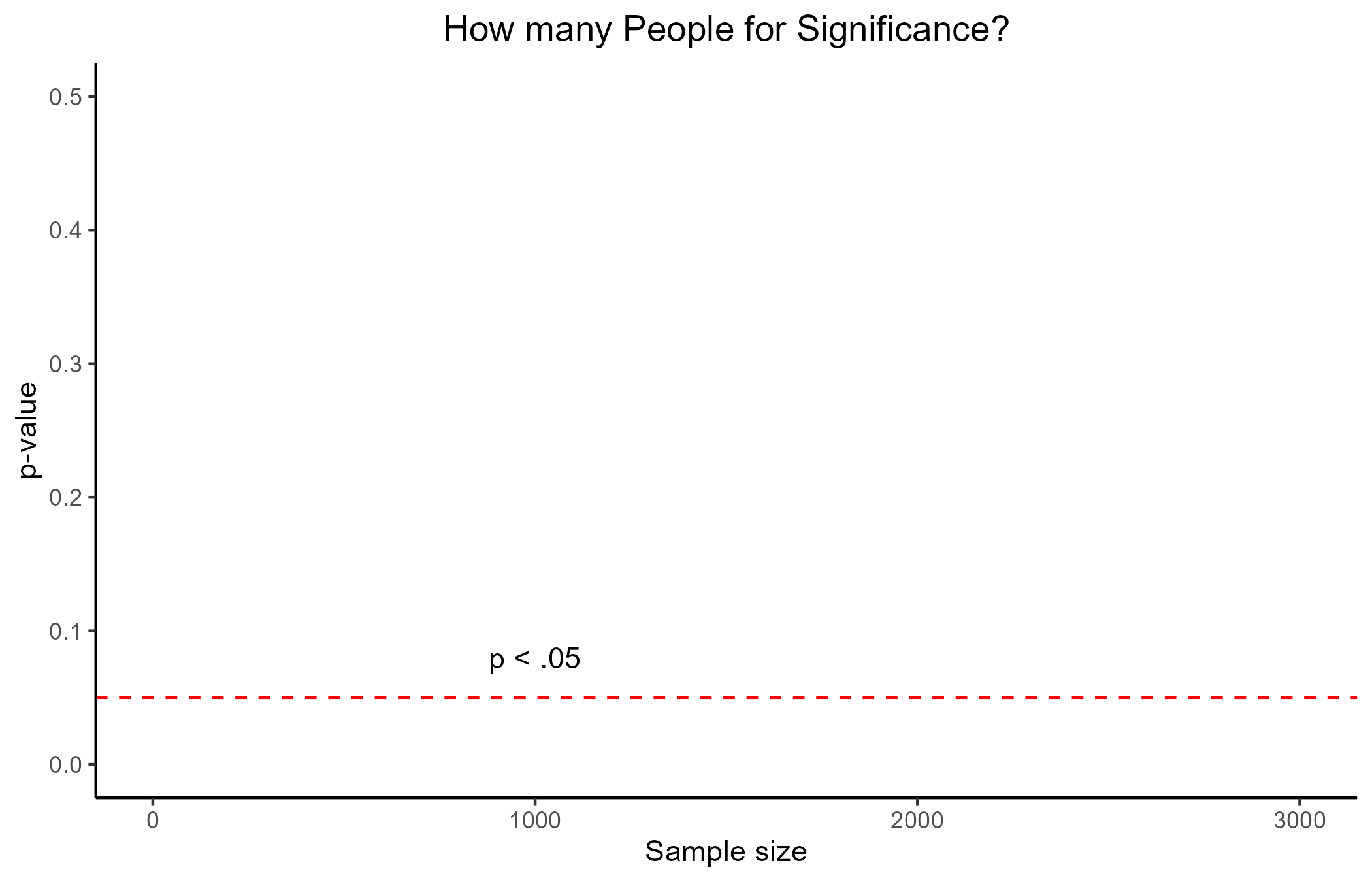
p-values? 😕
P-values are another often misunderstood, and frankly overemphasized, concept. We are taught that a p-value smaller than .05 (5% probability) is significant. The appropriate interpretation of p-values is as follows:
Assuming that my hypothesis is wrong (Null hypothesis), if I were to sample the same number of observations from the population an infinite number of times , what is the probability that I will observe the same results. (note that you can calculate a p-value for just about every statistic)
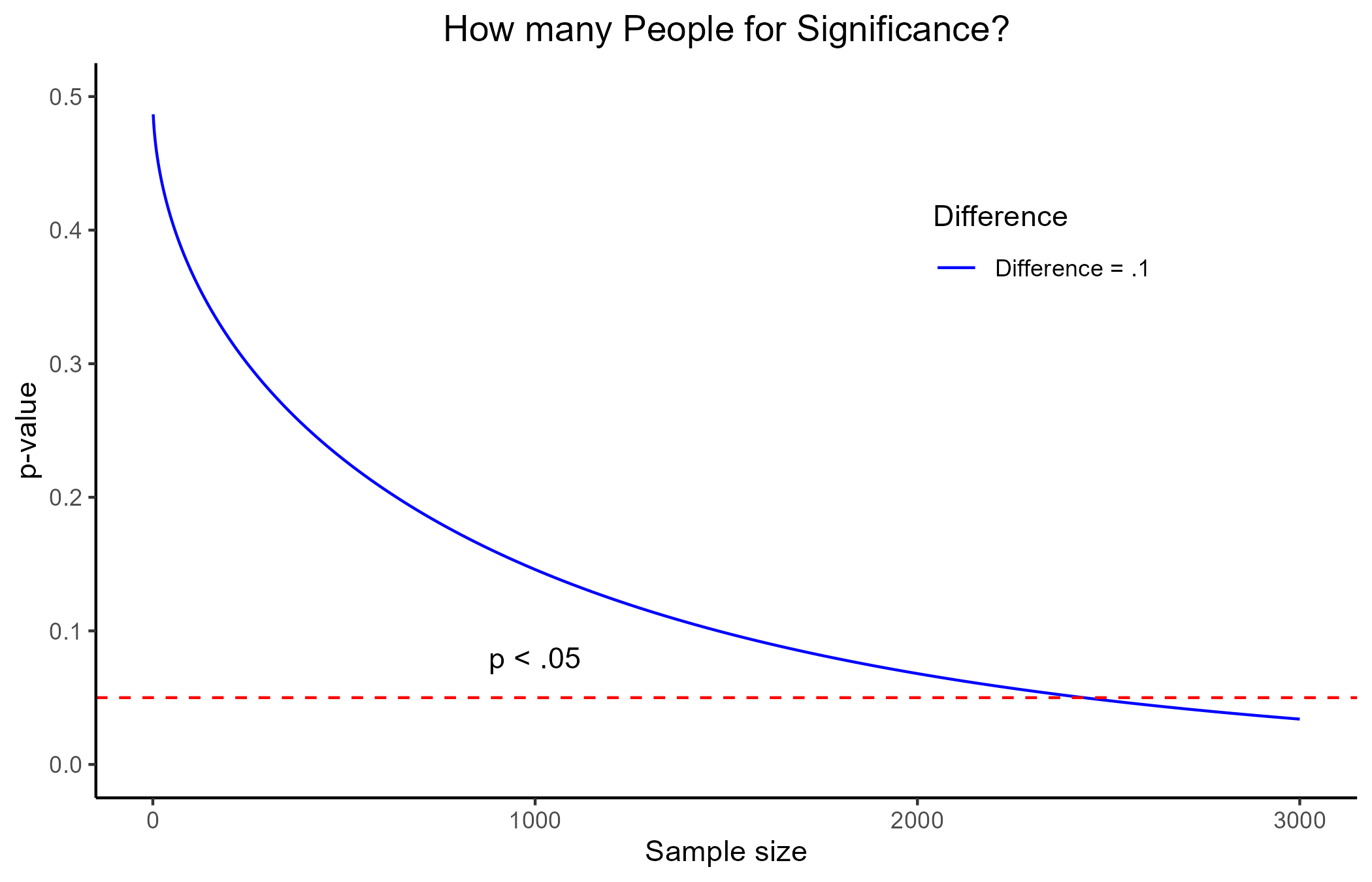
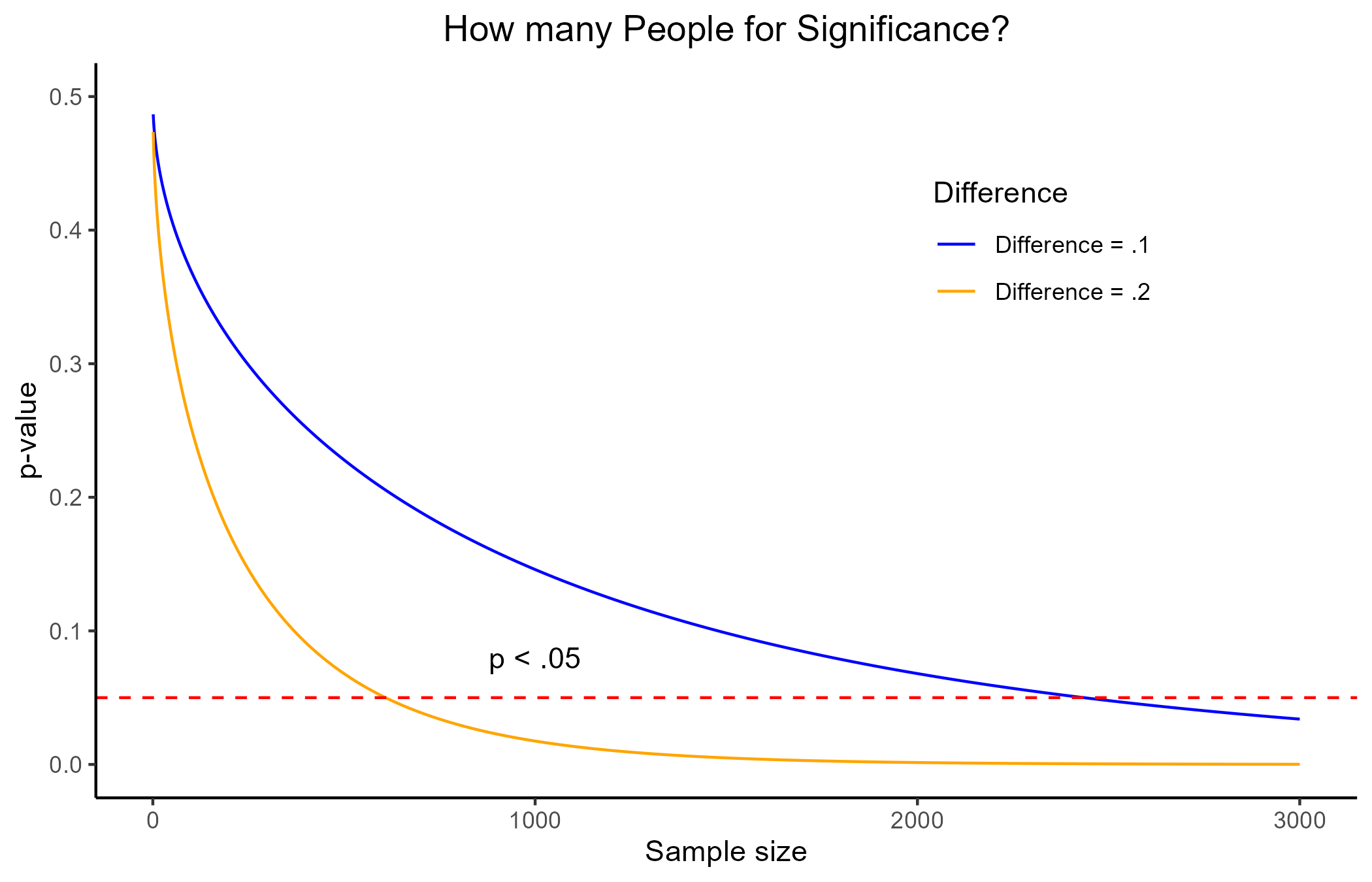
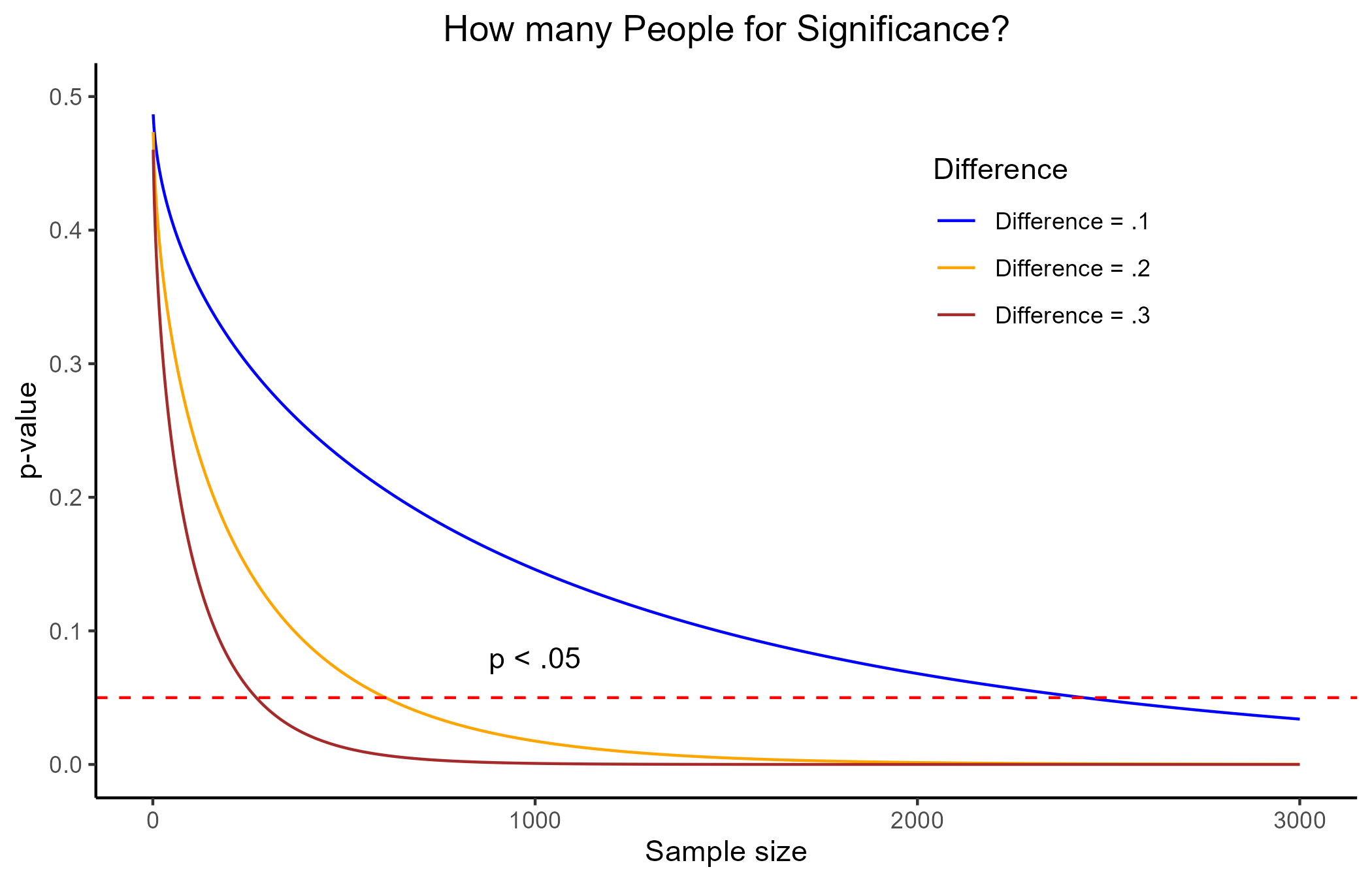
The main problem of p-values by themselves is that they carry no information about how different or how big the effect of the IV on the DV is. They main thing that influences p-values is sample size!
Let’s assume that we know that the average depression score in the population is 5 (SD = 3). Now, let’s say that we tried 3 different depression treatments for 3 different groups and found that, after treatment, these groups scores in depression respectively were: 4.9, 4.8, 4.7.
In this case, even with a difference as small as .3, the p-value will turn out significant with a sample size of around 270 people. Given the standard deviation of 3, a mean difference of .3 is laughable in practice!
Any Questions? 🤔

…And Class is over!🙃