A <- rbind(c(1,2),
           c(3,4),
           c(5,6))
B <- rbind(c(-9,-8),
           c(-7,-6))
A %*% B
[,1] [,2]
[1,] -23 -20
[2,] -55 -48
[3,] -87 -76Many models involve linear combinations of terms. For example, we already saw that the naïve Bayes classifier is the sum of weights of evidence. More generally, a naïve Bayes classifier has the form of a linear combination like \[ f(\mathbf{x})=\beta_0+h_1(\mathbf{x})+h_2(\mathbf{x})+\ldots+h_d(\mathbf{x}) \] Even decision trees can be written in this form. \[ f(\mathbf{x})=\beta_1I(\mathrm{age}<16)I(\mathrm{SES}>2)+\beta_2I(\mathrm{age}<16)I(\mathrm{SES}\leq 2) + \beta_3I(\mathrm{age}\geq 16) \] The classic linear model is \[ f(\mathbf{x})=\beta_0+\beta_1x_1+\beta_2x_2+\ldots+\beta_dx_d \] This is probably the most widely used model ever.
It gets tiresome to write this equation out each time. This is where linear algebra becomes handy. Let \[ \begin{split} \beta&= \begin{bmatrix} \beta_0 \\ \beta_1 \\ \vdots \\ \beta_d \end{bmatrix} \\ \mathbf{x}&= \begin{bmatrix} 1 \\ x_1 \\ \vdots \\ x_d \end{bmatrix} \end{split} \] These are column vectors, stacking all the \(\beta_j\)s on top of each other to form \(\beta\) and stacking all the features of a single observation, the \(x_j\)s, to form \(\mathbf{x}\). By default, all vectors are assumed to be column vectors (1 column, multiple rows). Both \(\beta\) and \(\mathbf{x}\) here are \((d+1)\times 1\) matrices.
The transpose operator flips rows and columns. \[ \begin{split} \beta' = \beta^T = \begin{bmatrix} \beta_0 & \beta_1 & \cdots & \beta_d \end{bmatrix} \end{split} \]
Two matrices, \(\mathbf{A}\) and \(\mathbf{B}\), can be multiplied if the number of columns in \(\mathbf{A}\) equals the number of rows in \(\mathbf{B}\). Matrix multiplication proceeds by summing the products of each row of \(\mathbf{A}\) with each column in \(\mathbf{B}\). We will work across the rows of \(\mathbf{A}\) and down the columns of \(\mathbf{B}\).
\[ \begin{split} \hspace{-1in} \begin{bmatrix} 1 & 2 \\ 3 & 4 \\ 5 & 6 \end{bmatrix} \begin{bmatrix} -9 & -8 \\ -7 & -6 \end{bmatrix} &= \begin{bmatrix} 1\times -9 + 2\times -7 & 1\times -8 + 2\times -6 \\ 3\times -9 + 4\times -7 & 3\times -8 + 4\times -6 \\ 5\times -9 + 6\times -7 & 5\times -8 + 6\times -6 \end{bmatrix}\\ &= \begin{bmatrix} -23 & -20 \\ -55 & -48 \\ -87 & -76 \end{bmatrix} \end{split} \]
We always use computers for matrix operations. In R, the %*% operator means matrix multiplication.
A <- rbind(c(1,2),
c(3,4),
c(5,6))
B <- rbind(c(-9,-8),
c(-7,-6))
A %*% B [,1] [,2]
[1,] -23 -20
[2,] -55 -48
[3,] -87 -76Compute \(\mathbf{A}\mathbf{B}\) for the following. First try by hand, then check your answers using R.
\[\mathbf{A}= \begin{bmatrix} -1 & 1 \\ 1 & -1 \end{bmatrix}, \; \mathbf{B}= \begin{bmatrix} 2 & 0 \\ 1 & 6 \end{bmatrix} \]
\[\mathbf{A}= \begin{bmatrix} 2 & 0 \\ 1 & 6 \end{bmatrix}, \; \mathbf{B}= \begin{bmatrix} -1 & 1 \\ 1 & -1 \end{bmatrix} \]
\[\mathbf{A}= \begin{bmatrix} 1 & 0 & 0 \\ 0 & 1 & 0 \\ 0 & 0 & 1 \end{bmatrix}, \; \mathbf{B}= \begin{bmatrix} 3 & 1 \\ 2 & 1 \\ 1 & 3 \end{bmatrix}\]
\[\mathbf{A}= \begin{bmatrix} 1 & 2 & 3 \end{bmatrix}, \hspace{0.1in} \mathbf{B}= \begin{bmatrix} 1 \\ 2 \\ 3 \end{bmatrix} \]
Here is R code for creating the matrices and multiplying then.
A <- rbind(c(-1,1),c(1,-1))
B <- rbind(c(2,0),c(1,6))
A %*% B
[,1] [,2]
[1,] -1 6
[2,] 1 -6A <- rbind(c(2,0),c(1,6))
B <- rbind(c(-1,1),c(1,-1))
A %*% B [,1] [,2]
[1,] -2 2
[2,] 5 -5A <- diag(1,3) # diagonal, or
A <- diag(c(1,1,1))
B <- cbind(c(3,2,1),c(1,1,3))
A %*% B [,1] [,2]
[1,] 3 1
[2,] 2 1
[3,] 1 3A <- matrix(1:3, ncol=3)
B <- t(A)
A %*% B [,1]
[1,] 14Some things to note from these exercises:
Matrix multiplication does not commute, \(\mathbf{AB}\neq\mathbf{BA}\)
The matrix with 1s on the diagonal and 0s everywhere else is the identity matrix, the matrix equivalent of multiplying by 1. Often denoted as \(\mathbf{I}\)
If you multiply a column vector by its transpose, it is the same as computing the sum of the squares of the elements, \(\mathbf{a}'\mathbf{a}=\sum a_i^2\).
We can now rewrite the long linear combination of features compactly. \[ \begin{split} \beta' &= \begin{bmatrix} \beta_0 & \beta_1 & \cdots & \beta_d \end{bmatrix} \\ \mathbf{x}'&= \begin{bmatrix} 1 & x_1 & \cdots & x_d \end{bmatrix} \\ \beta'\mathbf{x} &= \beta_0+\beta_1x_1+\beta_2x_2+\ldots+\beta_dx_d \end{split} \]
We are going to work through how to select \(\beta\) to minimize squared error, \[ J(\beta)= \sum_{i=1}^n (y_i-\beta'\mathbf{x}_i)^2 \] where \(\mathbf{x}_i\) is a column vector containing all the features for observation \(i\). Instead of having \(n\) separate vectors \(\mathbf{x}_i\), stack them all into one matrix, \(\mathbf{X}\). \[ \mathbf{X} = \begin{bmatrix} 1 & x_{11} & x_{12} & \cdots & x_{1d} \\ 1 & x_{21} & x_{22} & \cdots & x_{2d} \\ 1 & x_{31} & x_{32} & \cdots & x_{3d} \\ & & \vdots \\ 1 & x_{n1} & x_{n2} & \cdots & x_{nd} \\ \end{bmatrix} \] In this way \(\mathbf{X}\beta\) is \[ \mathbf{X}\beta = \begin{bmatrix} 1 & x_{11} & x_{12} & \cdots & x_{1d} \\ 1 & x_{21} & x_{22} & \cdots & x_{2d} \\ 1 & x_{31} & x_{32} & \cdots & x_{3d} \\ & & \vdots \\ 1 & x_{n1} & x_{n2} & \cdots & x_{nd} \\ \end{bmatrix} \begin{bmatrix} \beta_0 \\ \beta_1 \\ \vdots \\ \beta_d \end{bmatrix} = \begin{bmatrix} \beta'\mathbf{x}_1 \\ \beta'\mathbf{x}_2 \\ \vdots \\ \beta'\mathbf{x}_n \end{bmatrix} \] So \(\mathbf{X}\beta\) is a compact way of writing all of the predicted values for every observation in the dataset.
We can let \[ \mathbf{y} = \begin{bmatrix} y_1 \\ y_2 \\ \vdots \\ y_n \end{bmatrix} \] Then the differences between the actual and predicted values are \[ \mathbf{y} -\mathbf{X}\beta = \begin{bmatrix} y_1 \\ y_2 \\ \vdots \\ y_n \end{bmatrix} - \begin{bmatrix} \beta'\mathbf{x}_1 \\ \beta'\mathbf{x}_2 \\ \vdots \\ \beta'\mathbf{x}_n \end{bmatrix} = \begin{bmatrix} y_1-\beta'\mathbf{x}_1 \\ y_2-\beta'\mathbf{x}_2 \\ \vdots \\ y_n-\beta'\mathbf{x}_n \end{bmatrix} \] Remember in one of the exercises above you saw that \[ \begin{bmatrix} 1 & 2 & 3 \end{bmatrix} \begin{bmatrix} 1 \\ 2 \\ 3 \end{bmatrix} = 1^2+2^2+3^2 \] More generally \[ \mathbf{a}'\mathbf{a} = \sum_{i=1}^n a_i^2 \] That means we can rewrite the sum of squared error as \[ J(\beta)=(\mathbf{y} -\mathbf{X}\beta)'(\mathbf{y} -\mathbf{X}\beta) \]
To multiply this out we need some additional properties of the matrix transpose.
\((\mathbf{a}-\mathbf{b})'=\mathbf{a}'-\mathbf{b}'\)
\((\mathbf{AB})'=\mathbf{B}'\mathbf{A}'\)
Using these properties we can write \[ \begin{split} J(\beta) &= (\mathbf{y} -\mathbf{X}\beta)'(\mathbf{y} -\mathbf{X}\beta)\\ &= (\mathbf{y}' - (\mathbf{X}\beta)')(\mathbf{y} -\mathbf{X}\beta) \\ &= (\mathbf{y}' - \beta'\mathbf{X}')(\mathbf{y} -\mathbf{X}\beta) \\ &= \mathbf{y}'(\mathbf{y} -\mathbf{X}\beta) - \beta'\mathbf{X}'(\mathbf{y} -\mathbf{X}\beta) \\ &= \mathbf{y}'\mathbf{y} - \mathbf{y}'\mathbf{X}\beta - \beta'\mathbf{X}'\mathbf{y} + \beta'\mathbf{X}'\mathbf{X}\beta \\ &= \mathbf{y}'\mathbf{y} - \mathbf{y}'\mathbf{X}\beta - (\beta'\mathbf{X}'\mathbf{y})' + \beta'\mathbf{X}'\mathbf{X}\beta \\ &= \mathbf{y}'\mathbf{y} - \mathbf{y}'\mathbf{X}\beta - \mathbf{y}'\mathbf{X}\beta + \beta'\mathbf{X}'\mathbf{X}\beta \\ &= \mathbf{y}'\mathbf{y} - 2\mathbf{y}'\mathbf{X}\beta + \beta'\mathbf{X}'\mathbf{X}\beta \end{split} \]
Now we would like to find the value \(\beta'=\begin{bmatrix}\beta_0 & \beta_1 & \cdots & \beta_d\end{bmatrix}\) that minimizes \(J(\beta)\). We need to solve \(J'(\beta)=0\).
\[ \begin{split} \frac{\partial}{\partial\mathbf{x}} \mathbf{A} &= \mathbf{0} \\ \frac{\partial}{\partial\mathbf{x}} \mathbf{A}\mathbf{x} &= \mathbf{A}' \\ \frac{\partial}{\partial\mathbf{x}} \mathbf{x}'\mathbf{A} &= \mathbf{A} \\ \frac{\partial}{\partial\mathbf{x}} \mathbf{x}'\mathbf{A}\mathbf{x} &= (\mathbf{A}+\mathbf{A}')\mathbf{x} \\ \frac{\partial}{\partial\mathbf{x}} \mathbf{x}'\mathbf{A}\mathbf{x} &= 2\mathbf{A}\mathbf{x}, \;\mbox{ if $\mathbf{A}$ is symmetric} \end{split} \]
Example 1. Let’s walk through what it means for \(\frac{\partial}{\partial\mathbf{x}} \mathbf{A}\mathbf{x} = \mathbf{A}'\). Let \(\mathbf{A}=\begin{bmatrix} 1 & 2 & 3 \end{bmatrix}\) and we will set \(\mathbf{x}=\begin{bmatrix} x_1 \\ x_2 \\ x_3 \end{bmatrix}\)
\[ \begin{split} \frac{\partial}{\partial\mathbf{x}} \mathbf{A}\mathbf{x} &= \frac{\partial}{\partial\mathbf{x}} \begin{bmatrix} 1 & 2 & 3 \end{bmatrix}\begin{bmatrix} x_1 \\ x_2 \\ x_3 \end{bmatrix} \\ &= \frac{\partial}{\partial\mathbf{x}} x_1 + 2x_2 + 3x_3 \\ &= \begin{bmatrix} \frac{\partial}{\partial x_1} x_1 + 2x_2 + 3x_3 \\ \frac{\partial}{\partial x_2} x_1 + 2x_2 + 3x_3 \\ \frac{\partial}{\partial x_3} x_1 + 2x_2 + 3x_3\end{bmatrix} \\ &= \begin{bmatrix} 1 \\ 2 \\ 3 \end{bmatrix} \\ &= \mathbf{A}' \end{split} \]
Example 2. Let’s work through an example of \(\frac{\partial}{\partial\mathbf{x}} \mathbf{x}'\mathbf{A}\mathbf{x}\) to see that this works. \[ \begin{split} \frac{\partial}{\partial\mathbf{x}} \begin{bmatrix} x_1 & x_2 & x_3 \end{bmatrix} \begin{bmatrix} 3 & 1 & 0\\ 2 & 1 & 3\\ 1 & 3 & 1\\ \end{bmatrix} \begin{bmatrix} x_1 \\ x_2 \\ x_3 \end{bmatrix} \hspace{-2in}\\ &= \frac{\partial}{\partial\mathbf{x}} \begin{bmatrix} x_1 & x_2 & x_3 \end{bmatrix} \begin{bmatrix} 3x_1+x_2 \\ 2x_1+x_2+3x_3 \\ x_1+3x_2+x_3 \end{bmatrix} \\ &= \frac{\partial}{\partial\mathbf{x}} \begin{bmatrix} 3x_1^2+x_1x_2 + 2x_1x_2+x_2^2+3x_2x_3 + x_1x_3+3x_2x_3+x_3^2 \end{bmatrix}\\ &= \begin{bmatrix} 6x_1+x_2+2x_2+x_3 \\ x_1+2x_1+2x_2+3x_3 +3x_3\\ 3x_2+x_1+3x_2+2x_3 \end{bmatrix}\\ &= \begin{bmatrix} 6x_1+3x_2+x_3 \\ 3x_1+2x_2+6x_3\\ x_1+6x_2+2x_3 \end{bmatrix}\\ &= \begin{bmatrix} 6 & 3 & 1 \\ 3 & 2 & 6 \\ 1 & 6 & 2 \end{bmatrix} \begin{bmatrix} x_1 \\ x_2 \\ x_3 \end{bmatrix} \\ &= \left( \begin{bmatrix} 3 & 1 & 0\\ 2 & 1 & 3\\ 1 & 3 & 1\\ \end{bmatrix}+ \begin{bmatrix} 3 & 2 & 1\\ 1 & 1 & 3\\ 0 & 3 & 1\\ \end{bmatrix}\right) \begin{bmatrix} x_1 \\ x_2 \\ x_3 \end{bmatrix} \\ &= (\mathbf{A}+\mathbf{A}')\mathbf{x} \end{split} \]
We can now apply these properties to \(J(\beta)\). \[ \begin{split} \frac{\partial}{\partial\beta} J(\beta) &= \frac{\partial}{\partial\beta} \mathbf{y}'\mathbf{y} - 2\mathbf{y}'\mathbf{X}\beta + \beta'\mathbf{X}'\mathbf{X}\beta \\ &= -(2\mathbf{y}'\mathbf{X})' + (\mathbf{X}'\mathbf{X}+(\mathbf{X}'\mathbf{X})')\beta \\ &= -2\mathbf{X}'\mathbf{y} + (\mathbf{X}'\mathbf{X}+\mathbf{X}'\mathbf{X})\beta \\ &= -2\mathbf{X}'\mathbf{y} + 2\mathbf{X}'\mathbf{X}\beta \end{split} \] Now find \(\hat\beta\) so that \(J(\hat\beta)=0\). \[ \begin{split} -2\mathbf{X}'\mathbf{y} + 2\mathbf{X}'\mathbf{X}\hat\beta &= 0 \\ \mathbf{X}'\mathbf{X}\hat\beta &= \mathbf{X}'\mathbf{y} \end{split} \] Now it seems like we need to “divide” both sides by \(\mathbf{X}'\mathbf{X}\).
The inverse of a matrix, \(\mathbf{A}\), is the matrix that when multiplied with \(\mathbf{A}\) yields the identity matrix \(I\). That is, \[ A^{-1}A=I \]
If \(A=\begin{bmatrix} 2 & 0 \\ 1 & 6 \end{bmatrix}\), show that \(\mathbf{A}^{-1}=\begin{bmatrix} \frac{1}{2} & 0 \\ -\frac{1}{12} & \frac{1}{6} \end{bmatrix}\) by multiplying these two together.
First try to do this by hand. Then you can use R to confirm. R computes the inverse of a matrix using solve().
    A <- rbind(c(2,0), c(1,6))
    solve(A)
[,1] [,2]
[1,] 0.50000000 0.0000000
[2,] -0.08333333 0.1666667 # confirm it's an inverse
A %*% solve(A) [,1] [,2]
[1,] 1 0
[2,] 0 1While we know that division by 0 is a problem, for matrices there are many situations for which there is no inverse. Specifically, if one row (or column) can be written as a linear combination of other rows (or columns), then there is no inverse. There are some generalizations of inverses for these cases.
Now we can finish solving \[ \begin{split} \mathbf{X}'\mathbf{X}\hat\beta &= \mathbf{X}'\mathbf{y} \\ (\mathbf{X}'\mathbf{X})^{-1}\mathbf{X}'\mathbf{X}\hat\beta &= (\mathbf{X}'\mathbf{X})^{-1}\mathbf{X}'\mathbf{y} \\ \hat\beta &= (\mathbf{X}'\mathbf{X})^{-1}\mathbf{X}'\mathbf{y} \end{split} \] This is the classic solution to the least squares estimation problem. Some variants of this solution were known to the ancient Chinese and in the Arab world. A clear description of the problem and solution arrived with Legendre in 1805, but the matrix representation we use today probably did not appear until the early 1900s. In the last 100 years, this equation and its variations have driven a lot of scientific efforts.
Let’s use the prediction of age at death from the aspartic acid ratio example to test out our estimator for \(\hat\beta\). First, let’s use lm() to see what R’s built in regression function produces.
dAge <- data.frame(ratio=c(0.040,0.070,0.070,0.075,0.080,0.085,0.105,0.110,0.115,
                           0.130,0.140,0.150,0.160,0.165,0.170),
                   age=c(0,2,16,10,18,19,16,21,21,25,26,28,34,39,40))
lm(age~ratio, data=dAge)
Call:
lm(formula = age ~ ratio, data = dAge)

Coefficients:
(Intercept)        ratio
     -9.378      273.680
Now let’s assemble our design matrix \(\mathbf{X}\) from our dataset. We need to cbind() a column of 1s with the column containing the ratio data.
X <- cbind(1, dAge$ratio)
X
[,1] [,2]
[1,] 1 0.040
[2,] 1 0.070
[3,] 1 0.070
[4,] 1 0.075
[5,] 1 0.080
[6,] 1 0.085
[7,] 1 0.105
[8,] 1 0.110
[9,] 1 0.115
[10,] 1 0.130
[11,] 1 0.140
[12,] 1 0.150
[13,] 1 0.160
[14,] 1 0.165
[15,] 1 0.170Then let’s set y to be our outcome vector
y <- dAge$age
y
[1] 0 2 16 10 18 19 16 21 21 25 26 28 34 39 40Finally, let’s use R to compute \((\mathbf{X}'\mathbf{X})^{-1}\mathbf{X}'\mathbf{y}\). Remember that t() is for matrix transpose and solve() computes the matrix inverse.
# compute (X'X)^-1X'y
betaHat <- solve(t(X) %*% X) %*% t(X) %*% y
betaHat
[,1]
[1,] -9.378437
[2,] 273.679616Excellent! It produces the same estimate for \(\hat\beta\) as the lm() function.
Want to go down the rabbit hole and learn about all the gory details about how R fits ordinary least squares? Visit this deep dive.
We started with a very general functional form for the predictive model \[ f(\mathbf{x})=\beta_0+h_1(\mathbf{x})+h_2(\mathbf{x})+\ldots+h_d(\mathbf{x}) \] Even if \(\mathbf{x}\) is univariate, we can let the \(h_j(x)\) be more complex functions of \(x\), polynomials, for example. \[ f(x)=\beta_0+\beta_1x+\beta_2 x^2+\beta_3 x^3 + \ldots + \beta_d x^d \] If we let \(d\) get too large relative to the number of observations, then eventually there are multiple polynomials that can completely connect the dots. The predictive model can also be wildly fluctuating. Regularization is a key strategy to prevent this.
The simplest regularization is simply to limit the size of \(d\). Regularization basically limits the capacity of the model to fit complex shapes. At the extreme end, limiting \(d=1\) results in the familiar linear model. However, what if there really needs to be an \(x^4\) term but an \(x^2\) term is less important.
Ridge regression proposes changing the objective function to be \[ J(\beta)= \sum_{i=1}^n (y_i-\beta'\mathbf{x}_i)^2 + \lambda\sum_{j=1}^d \beta_j^2 \] This says that we should evaluate \(\beta\) by how small it makes the sum of squared error, but penalize the model if doing so requires very large values for \(\beta\). The penalty is sometimes called a “ridge” penalty or an \(L_2\) penalty. If we set \(\lambda\) to be a very large number, then this \(J\) will be very large if there are any non-zero \(\beta_j\). There is always a \(\lambda\) large enough to make exist a unique \(\beta\) that minimizes \(J\).
Let us use our linear algebra skills to find a solution for the optimal \(\beta\) for a fixed value of \(\lambda\). \[ \begin{split} \frac{\partial}{\partial\beta}\,J(\beta) &= \frac{\partial}{\partial\beta}\,\left(\sum_{i=1}^n (y_i-\beta'\mathbf{x}_i)^2 + \lambda\sum_{j=1}^d \beta_j^2\right) \\ &= \frac{\partial}{\partial\beta}\,\left(\mathbf{y}'\mathbf{y} - 2\mathbf{y}'\mathbf{X}\beta + \beta'\mathbf{X}'\mathbf{X}\beta +\lambda\beta'\beta\right) \\ &= \frac{\partial}{\partial\beta}\,\left(\mathbf{y}'\mathbf{y} - 2\mathbf{y}'\mathbf{X}\beta + \beta'\mathbf{X}'\mathbf{X}\beta +\lambda\beta'\mathbf{I}\beta\right) \\ &= \frac{\partial}{\partial\beta}\,\left(\mathbf{y}'\mathbf{y} - 2\mathbf{y}'\mathbf{X}\beta + \beta'(\mathbf{X}'\mathbf{X} +\lambda\mathbf{I})\beta\right) \\ &= - 2\mathbf{X}'\mathbf{y} + 2(\mathbf{X}'\mathbf{X}+\lambda\mathbf{I})\beta \\ \hat\beta_\mathrm{ridge} &= (\mathbf{X}'\mathbf{X}+\lambda\mathbf{I})^{-1}\mathbf{X}'\mathbf{y} \end{split} \] The squared penalty on the \(\beta_j\)s has the effect of adding \(\lambda\) to the diagonal of the \(\mathbf{X}'\mathbf{X}\) matrix (this is where the term ridge regression comes from). Even if \(\mathbf{X}'\mathbf{X}\) does not have an inverse, there is some value of \(\lambda\) that will make \(\mathbf{X}'\mathbf{X}+\lambda\mathbf{I}\) invertible.
Regularization plays a major role in machine learning. It will take different forms depending on the machine learning method. For decision trees we controlled the number of terminal nodes. For linear models we can select the degree of the polynomial or set a ridge penalty to shrink the capacity of the method to capture complex patterns.
Here let’s simulate some data with a little bit of curvature in the relationship between \(x\) and \(y\).
set.seed(20240225)
x <- seq(0,1,length.out=40)
y <- sin(6*x) + rnorm(length(x),0,0.7)
Let’s use least squares to fit a 10-degree polynomial to this pattern. I also threw in a square root term too. This means that we will estimate 12 coefficients to fit to these 40 observations. The function I() in the model.matrix() call below is an “inhibitor” function in R. It prevents R from interpreting formula terms in any other way than just basic math operations. This is necessary because ^ has a special meaning in R formulas.
X <- model.matrix(~x+I(x^2)+I(x^3)+I(x^4)+I(x^5)+I(x^6)+I(x^7)+I(x^8)+I(x^9)+
                    I(x^10)+sqrt(x),
                  data=data.frame(x))

betaHat <- solve(t(X) %*% X) %*% t(X) %*% y
yHat <- X %*% betaHat
plot(x,y)
lines(x, yHat, col="#E69F00", lwd=3)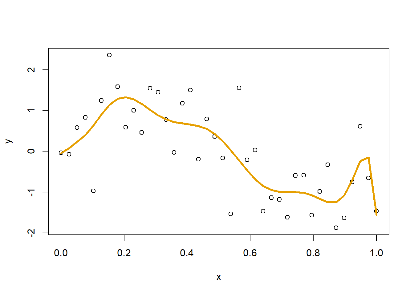
The resulting fit is not bad, but there is a weird bend at the far right. Also weird is the magnitude of some of the coefficients, with some exceeding 1,000,000.
betaHat [,1]
(Intercept) -4.284778e-02
x 6.222010e+01
I(x^2) -1.104704e+03
I(x^3) 1.377847e+04
I(x^4) -9.347079e+04
I(x^5) 3.650949e+05
I(x^6) -8.647856e+05
I(x^7) 1.263112e+06
I(x^8) -1.111730e+06
I(x^9) 5.405930e+05
I(x^10) -1.115453e+05
sqrt(x) -5.879676e+00Let’s try a little ridge regression. I’ll plot the originally estimated curve in orange, in teal green will be a curve with a tiny \(\lambda\) of 0.0001, blue will have a \(\lambda\) of 0.05, and in black will be a curve with \(\lambda\) set very large at 1000. Note that I have zeroed out the squared penalty on \(\beta_0\) so that the squared penalty only applies to the coefficients on terms with \(x\).
plot(x,y)

# the identity matrix... but with a 0 in the top left to avoid a
#   penalty on beta0
matI <- diag(c(0,rep(1,ncol(X)-1)))
lambda <- 0
betaHat <- solve(t(X) %*% X + lambda*matI) %*% t(X) %*% y
yHat <- X %*% betaHat
lines(x, yHat, col="#E69F00", lwd=3)

lambda <- 0.0001
betaHat <- solve(t(X) %*% X + lambda*matI) %*% t(X) %*% y
yHat <- X %*% betaHat
lines(x, yHat, col="#009E73", lwd=3)

lambda <- 0.05
betaHat <- solve(t(X) %*% X + lambda*matI) %*% t(X) %*% y
yHat <- X %*% betaHat
lines(x, yHat, col="#0072B2", lwd=3)

lambda <- 1000
betaHat <- solve(t(X) %*% X + lambda*matI) %*% t(X) %*% y
yHat <- X %*% betaHat
lines(x, yHat, col="black", lwd=3)

legend(0.7, 2.2,
       legend = c(bquote(lambda == 0),
                  bquote(lambda == .(sprintf("%.4f", 0.0001))),
                  bquote(lambda == 0.05),
                  bquote(lambda == 1000)),
       col=c("#E69F00","#009E73","#0072B2","black"),
       lwd=3)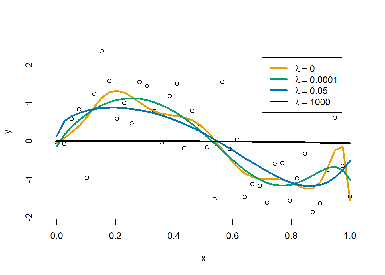
As the ridge penalty increases we get a smoother fit, but too much of a penalty will result in a flat, horizontal line near \(y=0\).
We can trace out what happens to the coefficients as we increase \(\lambda\). The following plot follows the paths of the \(\beta\)s as I change \(\lambda\) from 0.0001 to 0.1. I’ve run the generation of the \(\lambda\)s on the square root scale so that we get more \(\lambda\)s near 0.0001 and fewer near 0.1.
lambda <- seq(sqrt(0.0001),sqrt(0.1), length=30); lambda <- lambda^2

betas <- matrix(NA, nrow=length(betaHat), ncol=length(lambda))

for(i in 1:length(lambda))
{
  betas[,i] <- solve(t(X) %*% X + lambda[i]*matI) %*% t(X) %*% y
}
plot(lambda,lambda,
     ylim=range(betas),
     ylab=expression(beta),
     xlab=expression(lambda),
     type="n")

color_palette <- viridis::cividis(11)
for(i in 1:nrow(betas))
{
  lines(lambda, betas[i,],
        col=color_palette[i],
        lwd=2)
}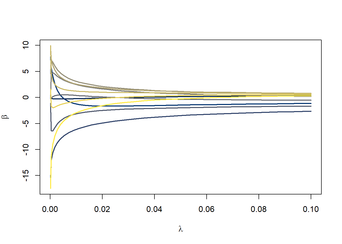
In general, you can see that the coefficients are getting squeezed closer to 0 as \(\lambda\) increases. Eventually with a large enough value for \(\lambda\), they will all get squeezed to 0. In this example, just a modest amount of penalizing the coefficients results in a smoother, more stable fit to the data.
The sum of squared error is a quadratic function of \(\beta\). That made it easy to produce a simple formula for \(\hat\beta\). Most functionals, \(J\), do not have such a simple form.
In univariate calculus you learned about Taylor series. \[ J(x) = J(x_0) + J'(x_0)(x-x_0) + \frac{1}{2}J''(x_0)(x-x_0)^2 + \ldots \]
We are going to ignore the \(\ldots\) at the end and assume that our \(J\) can be well approximated by a quadratic. If we want to optimize this then we can compute \(\frac{dJ}{dx}=0\), using our quadratic approximation. \[ \begin{split} \frac{d}{dx} J(x) &= J'(x_0) + J''(x_0)(x-x_0) \\ \hat x &\leftarrow x_0-\frac{J'(x_0)}{J''(x_0)} \end{split} \]
This is “Newton’s method.”
Find \(p\) to optimize \[ \begin{split} J(p) &= x\log(p)+(n-x)\log(1-p) \\ J'(p) &= \frac{x}{p} - \frac{n-x}{1-p} \\ J''(p) &= -\frac{x}{p^2} - \frac{n-x}{(1-p)^2} \\ \hat p &\leftarrow \hat p - \frac{\frac{x}{\hat p} - \frac{n-x}{1-\hat p}}{-\frac{x}{\hat p^2} - \frac{n-x}{(1-\hat p)^2}} \end{split} \tag{1}\]
If \(x=10\), \(n=30\), and we initially guess \(\hat p=0.1\), then we get the sequence {0.1759036, 0.268295, 0.3246771, 0.3332151, 0.3333333}.
This is a little bit of overkill because we can set \(J'(p)=0\) and solve that \(\hat p=\frac{x}{n}\). Or if we start the last line of (1) at \(\hat p =\frac{1}{2}\), then you will get \(\hat p=\frac{x}{n}\) on the first iteration. The equation in the first line of (1) is the log likelihood function for estimating a binomial proportion, naturally optimized when you count the total number of “successes,” \(x\), out of \(n\) trials.
We observe data of the form \((\mathbf{x}_1,y_1), \ldots, (\mathbf{x}_n,y_n)\), where \(y_i \in \{0,1\}\). We assume \(y_i \sim \mathrm{Bern}(p_i)\) where, shortly, we will connect \(p_i\) to depend on \(\mathbf{x}_i\).
The probability of observing a specific sequence of \(y_i\)s is \[ \prod_{i=1}^n p_i^{y_i}(1-p_i)^{1-y_i} \]
On the log scale \[ \begin{split} \log\prod_{i=1}^n p_i^{y_i}(1-p_i)^{1-y_i} &= \sum_{i=1}^n y_i\log p_i + (1-y_i)\log(1-p_i) \\ &= \sum_{i=1}^n y_i(\log p_i -\log(1-p_i)) + \log(1-p_i) \\ &= \sum_{i=1}^n y_i\log\frac{p_i}{1-p_i} + \log(1-p_i) \end{split} \tag{2}\]
The log-likelihood has the \(y_i\) multiplied by the log odds. This is the primary reason we model the probability of an outcome on the log odds scale. The log odds function is known as the “canonical link function” for logistic regression. Logistic regression assumes that \[ \log\frac{p_i}{1-p_i} = \beta'\mathbf{x}_i \]
We will also need the inverse of the log odds, called the inverse logit function, the standard logistic function, or the sigmoid function. \[ p_i = \frac{1}{1+e^{-\beta'\mathbf{x}_i}} \]
Substituting into the last line of (2) we get \[ \begin{split} \ell(\beta) &= \sum_{i=1}^n y_i\beta'\mathbf{x}_i + \log\left(1-\frac{1}{1+e^{-\beta'\mathbf{x}_i}}\right) \\ &= \sum_{i=1}^n y_i\beta'\mathbf{x}_i + \log\left(\frac{e^{-\beta'\mathbf{x}_i}}{1+e^{-\beta'\mathbf{x}_i}}\right) \\ &= \sum_{i=1}^n y_i\beta'\mathbf{x}_i + \log\left(\frac{e^{-\beta'\mathbf{x}_i}}{1+e^{-\beta'\mathbf{x}_i}}\frac{e^{\beta'\mathbf{x}_i}}{e^{\beta'\mathbf{x}_i}}\right) \\ &= \sum_{i=1}^n y_i\beta'\mathbf{x}_i + \log\left(\frac{1}{1+e^{\beta'\mathbf{x}_i}}\right) \\ &= \sum_{i=1}^n y_i\beta'\mathbf{x}_i - \log\left(1+e^{\beta'\mathbf{x}_i}\right) \end{split} \]
There is no closed form solution to \(\ell'(\beta)=0\). Instead, we need a numerical method for finding the \(\hat\beta\) that maximizes \(\ell(\beta)\).
We previously saw that we can use the Taylor series expansion of \(J(\beta)\) to approximate it and use Newton’s method to optimize it. \[ J(\beta) \approx J(b) + J'(b)(\beta-b) + \frac{1}{2}J''(b)(\beta-b)^2 \tag{3}\]
If this approximation is good, that is, \(J(\beta)\) is well approximated by a parabola, then we can find the \(\beta\) to maximize \(J(\beta)\). Take a derivative of (3) with respect to \(\beta\) and set it equal to 0. \[ \begin{split} J'(\beta) &\approx J'(b)+J''(b)(\beta-b) \\ J'(\hat\beta) &= 0 \\ J'(b)+J''(b)(\hat\beta-b) &= 0 \\ \hat\beta &= b - \frac{J'(b)}{J''(b)} \end{split} \tag{4}\] If we initiate \(b\) as a guess for the \(\beta\) that maximizes \(J(\beta)\), then (4) will produce a better guess for \(\hat\beta\)… typically. We can iterate (4) several times until convergence to give us the maximizer of \(J(\beta)\).
The multivariate Taylor expansion gives a generalization of this approach. \[ \begin{split} J(\boldsymbol\beta) &\approx J(\mathbf{b}) + (\boldsymbol\beta-\mathbf{b})' \begin{bmatrix} \frac{\partial J}{\partial\beta_0} \\ \vdots \\ \frac{\partial J}{\partial\beta_d} \end{bmatrix} + \frac{1}{2}(\boldsymbol\beta-\mathbf{b})' \begin{bmatrix} \frac{\partial^2 J}{\partial\beta_0^2} & \cdots & \frac{\partial^2 J}{\partial\beta_0\partial\beta_d} \\ \vdots & \vdots & \vdots \\ \frac{\partial^2 J}{\partial\beta_0\partial\beta_d} & \cdots & \frac{\partial^2 J}{\partial\beta_d^2} \end{bmatrix}(\boldsymbol\beta-\mathbf{b}) \\ &= J(\mathbf{b}) + (\boldsymbol\beta-\mathbf{b})'\mathbf{G} + \frac{1}{2}(\boldsymbol\beta-\mathbf{b})'\mathbf{H}(\boldsymbol\beta-\mathbf{b}) \\ &= J(\mathbf{b}) + \boldsymbol\beta'\mathbf{G}-\mathbf{b}'\mathbf{G} + \frac{1}{2}(\boldsymbol\beta-\mathbf{b})'\mathbf{H}(\boldsymbol\beta-\mathbf{b}) \\ \frac{\partial}{\partial\beta} J(\boldsymbol\beta) &= 0 + \mathbf{G} - 0 + \frac{1}{2}\cdot 2\mathbf{H}(\boldsymbol\beta-\mathbf{b}) \\ &= G+\mathbf{H}(\boldsymbol\beta-\mathbf{b}) \\ 0 &= G+\mathbf{H}(\boldsymbol{\hat\beta}-\mathbf{b}) \\ -\mathbf{H}(\boldsymbol{\hat\beta}-\mathbf{b}) &= G \\ \boldsymbol{\hat\beta}-\mathbf{b} &= -\mathbf{H}^{-1}G \\ \boldsymbol{\hat\beta} &= \mathbf{b}-\mathbf{H}^{-1}G \\ \boldsymbol{\hat\beta} &\leftarrow \boldsymbol{\hat\beta} - \mathbf{H}^{-1}\mathbf{G}\\ \end{split} \]
Where \(\mathbf{G}\) is a vector of first derivatives (that could be written as \(\nabla J\)), the score function, and \(\mathbf{H}\) is the matrix of second derivatives (could be written as \(\nabla^2 J\)), the Hessian or the negative Fisher information.
The first derivative, or gradient or “score function”, is \[ \begin{split} \frac{\partial}{\partial\beta} \ell(\beta) &= \frac{\partial}{\partial\beta}\sum_{i=1}^n y_i\beta'\mathbf{x}_i - \log\left(1+e^{\beta'\mathbf{x}_i}\right) \\ &= \sum_{i=1}^n y_i\mathbf{x}_i - \frac{e^{\beta'\mathbf{x}_i}}{1+e^{\beta'\mathbf{x}_i}}\mathbf{x}_i \\ &= \sum_{i=1}^n \mathbf{x}_i\left(y_i - \frac{e^{\beta'\mathbf{x}_i}}{1+e^{\beta'\mathbf{x}_i}}\frac{e^{-\beta'\mathbf{x}_i}}{e^{-\beta'\mathbf{x}_i}}\right) \\ &= \sum_{i=1}^n \mathbf{x}_i\left(y_i - \frac{1}{1+e^{-\beta'\mathbf{x}_i}}\right) \\ &= \sum_{i=1}^n \mathbf{x}_i(y_i - p_i) \\ &= \mathbf{X}'(\mathbf{y}-\mathbf{p}) \end{split} \]
The matrix of second derivatives, or Hessian matrix, is \[ \begin{split} \frac{\partial^2}{\partial\beta\,\partial\beta'} \ell(\beta)&= \frac{\partial}{\partial\beta} \sum_{i=1}^n \mathbf{x}_i\left(y_i - \frac{1}{1+e^{-\beta'\mathbf{x}_i}}\right) \\ &= \sum_{i=1}^n -\mathbf{x}_i \frac{\partial}{\partial\beta} (1+e^{-\beta'\mathbf{x}_i})^{-1} \\ &= \sum_{i=1}^n \mathbf{x}_i\frac{1}{(1+e^{-\beta'\mathbf{x}_i})^2}e^{-\beta'\mathbf{x}_i}(-\mathbf{x}_i') \\ &= -\sum_{i=1}^n \mathbf{x}_i\mathbf{x}_i'\frac{1}{1+e^{-\beta'\mathbf{x}_i}}\frac{e^{-\beta'\mathbf{x}_i}}{1+e^{-\beta'\mathbf{x}_i}} \\ &= -\sum_{i=1}^n \mathbf{x}_i\mathbf{x}_i'\frac{1}{1+e^{-\beta'\mathbf{x}_i}}\left(1-\frac{1}{1+e^{-\beta'\mathbf{x}_i}}\right) \\ &= -\sum_{i=1}^n \mathbf{x}_i\mathbf{x}_i'p_i(1-p_i) \\ &= -\mathbf{X}'\mathbf{W}\mathbf{X} \end{split} \] where \(\mathbf{W}\) is an \(n \times n\) diagonal matrix with \(p_i(1-p_i)\) on the diagonal.
Applying Newton-Raphson to the logistic regression score and Hessian yields \[ \begin{split} \hat\beta &\leftarrow \hat\beta - (-\mathbf{X}'\mathbf{W}\mathbf{X})^{-1}\mathbf{X}'(\mathbf{y}-\mathbf{p}) \\ &= \hat\beta + (\mathbf{X}'\mathbf{W}\mathbf{X})^{-1}\mathbf{X}'(\mathbf{y}-\mathbf{p}) \end{split} \tag{5}\]
Recall that when fitting an ordinary least squares regression, the least squares estimate of \(\hat\beta=(\mathbf{X}'\mathbf{X})^{-1}\mathbf{X}'\mathbf{y}\). Relatedly, if you are trying to fit a weighted least squares model to find the \(\hat\beta\) to minimize \[ \sum_{i=1}^n w_i(y_i-\beta'\mathbf{x}_i)^2 \]
then the solution is \(\hat\beta=(\mathbf{X}'\mathbf{W}\mathbf{X})^{-1}\mathbf{X}'\mathbf{W}\mathbf{y}\) where \(W\) is a diagonal matrix with \(w_i\) on the diagonal. (5) appears to be similar. With a little work we can rewrite (5) as a weighted least squares solution. \[ \begin{split} \hat\beta &\leftarrow \hat\beta + (\mathbf{X}'\mathbf{W}\mathbf{X})^{-1}\mathbf{X}'(\mathbf{y}-\mathbf{p}) \\ &= (\mathbf{X}'\mathbf{W}\mathbf{X})^{-1}\mathbf{X}'\mathbf{W}\mathbf{X}\hat\beta + (\mathbf{X}'\mathbf{W}\mathbf{X})^{-1}\mathbf{X}'(\mathbf{y}-\mathbf{p}) \\ &= (\mathbf{X}'\mathbf{W}\mathbf{X})^{-1}\mathbf{X}'(\mathbf{W}\mathbf{X}\hat\beta + \mathbf{y}-\mathbf{p}) \\ &= (\mathbf{X}'\mathbf{W}\mathbf{X})^{-1}\mathbf{X}'\mathbf{W}(\mathbf{X}\hat\beta + \mathbf{W}^{-1}(\mathbf{y}-\mathbf{p}))\\ &= (\mathbf{X}'\mathbf{W}\mathbf{X})^{-1}\mathbf{X}'\mathbf{W}\mathbf{z} \end{split} \]
where \(z_i=\hat\beta'\mathbf{x}_i +\frac{y_i-p_i}{p_i(1-p_i)}\) and is called the “working response.”
The Iteratively Reweighted Least Squares (IRLS) algorithm initiates \(\hat\beta\) to some reasonable guess (like all coefficients are 0 except for the intercept), computes \(p_i=\frac{1}{1+e^{-\hat\beta'\mathbf{x}_i}}\), sets weights to \(w_i=p_i(1-p_i)\), computes the working response \(z_i\), and then runs a standard weighted least squares procedures to obtain a better estimate of \(\hat\beta\). Then IRLS recomputes \(p_i\), \(w_i\), and \(z_i\) and repeats the process until convergences. Typically, IRLS converges in 3-4 iterations.
Let’s start by simulating some data where \(\beta=\begin{bmatrix} -1 & 1 & -1\end{bmatrix}\).
set.seed(20240217)
n <- 10000
beta <- c(-1,1,-1)
X <- cbind(1, matrix(runif(n*2), ncol=2))
y <- rbinom(n, 1, 1/(1+exp(-X %*% beta)))
Normally we would just run glm() with family=binomial to use R’s built in logistic regression estimation. Let’s run that now to see what we should get for \(\hat\beta\). Note that the -1 in the model formula tells R not to include an intercept term because I have already included a column of 1s in X.
glm1 <- glm(y~-1+X, family = binomial)
glm1
Call:  glm(formula = y ~ -1 + X, family = binomial)

Coefficients:
    X1      X2      X3
-1.044   1.087  -1.020

Degrees of Freedom: 10000 Total (i.e. Null);  9997 Residual
Null Deviance:      13860
Residual Deviance: 11430    AIC: 11440
Next let’s try to visualize what the 2D surface of the log-likelihood function looks like in the neighborhood of \(\hat\beta\).
logitLL <- function(beta, X0, y0)
{
   Xbeta <- X0 %*% beta
   return( as.numeric( y0 %*% Xbeta - sum(log(1+exp(Xbeta))) ))
}

beta0 <- coef(glm1)
bGrid <- expand.grid(beta0=beta0[1],
                     beta1=beta0[2] + seq(-3,3,length=201),
                     beta2=beta0[3] + seq(-3,3,length=201))
bGrid$LL <- apply(bGrid[,1:3], 1, logitLL, X0=X, y0=y)


plotLL <- list(x=beta0[2] + seq(-2,2,length=201),
               y=beta0[3] + seq(-2,2,length=201),
               z=matrix(bGrid$LL, nrow=201))
contour(x=plotLL,
        levels=c(pretty(bGrid$LL, 15), floor(max(bGrid$LL))))
points(coef(glm1)[2],coef(glm1)[3])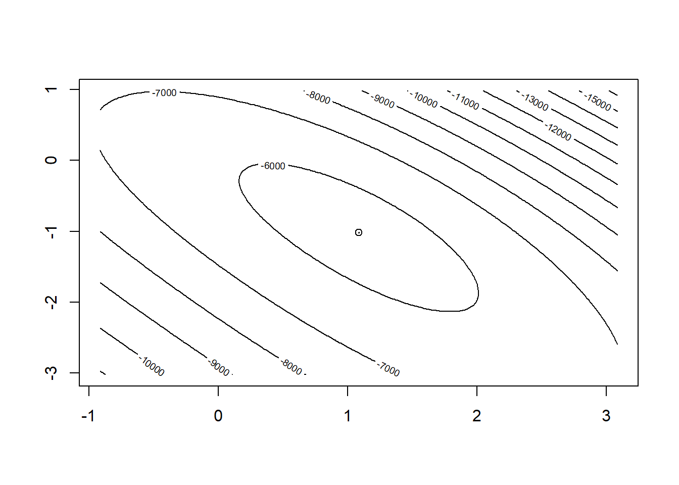
Now let’s assume we did not have access to R’s glm() and use our own Newton-Raphson algorithm to optimize the logistic regression log-likelihood. The orange dot is our current guess \(\hat\beta=\begin{bmatrix}0 & 0 & 0\end{bmatrix}\) and the orange line shows where the gradient is telling us we should head.
# starting value intercept only
beta0 <- c(log(mean(y)/(1-mean(y))), 0, 0)
contour(x=plotLL,
        levels=c(pretty(bGrid$LL, 15), floor(max(bGrid$LL))))
points(beta0[2], beta0[3], col="#E69F00", pch=16, cex=1.5)
points(coef(glm1)[2], coef(glm1)[3])

# (X'WX)^-1 X'(y-p) is the direction where Newton-Raphson tells us we should move
p <- as.numeric(1/(1+exp(-X %*% beta0)))
betaNew <- beta0 + solve(t(X) %*% diag(p*(1-p)) %*% X) %*% t(X) %*% (y-p)
lines(c(beta0[2],betaNew[2]), c(beta0[3],betaNew[3]), col="#E69F00", lwd=2)

beta0 <- betaNew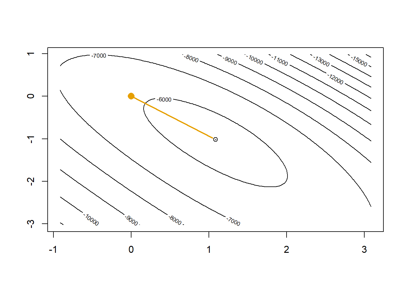
In one step we get very close to the maximum. A second step will get us to the top.
contour(x=plotLL,
        levels=c(pretty(bGrid$LL, 15), floor(max(bGrid$LL))))
points(beta0[2], beta0[3], col="#E69F00", pch=16, cex=1.5)
points(coef(glm1)[2],coef(glm1)[3])

# (X'WX)^-1 X'(y-p) is the direction where Newton-Raphson tells us we should move
p <- as.numeric(1/(1+exp(-X %*% beta0)))
betaNew <- beta0 + solve(t(X) %*% diag(p*(1-p)) %*% X) %*% t(X) %*% (y-p)
lines(c(beta0[2],betaNew[2]), c(beta0[3],betaNew[3]), col="#E69F00", lwd=2)

beta0 <- betaNew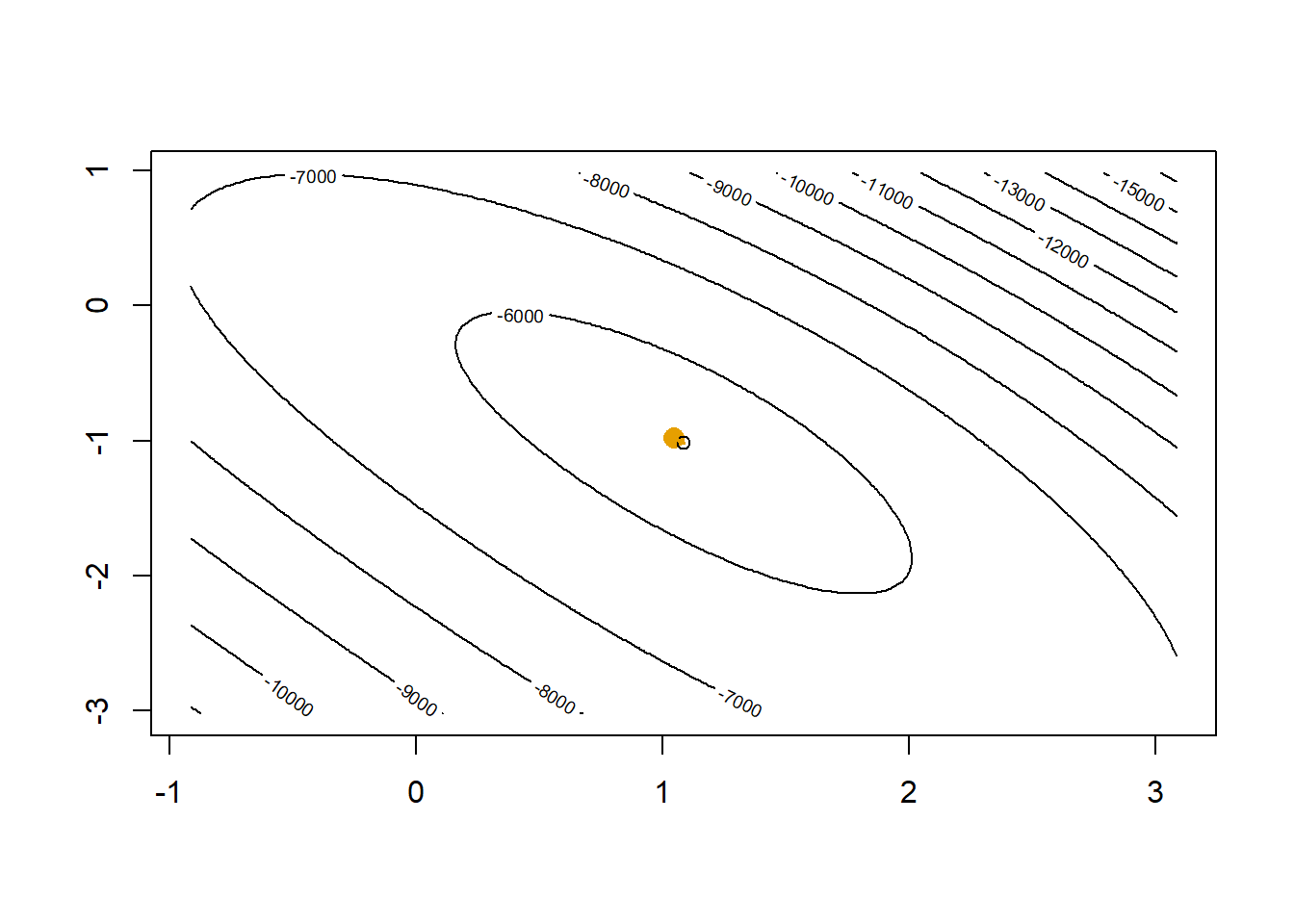
After two steps our Newton-Raphson gets us essentially to where glm() would get us.
cbind(beta0, coef(glm1)) [,1] [,2]
X1 -1.043583 -1.044113
X2 1.085888 1.086881
X3 -1.019002 -1.019929I showed that we can rewrite the Newton-Raphson algorithm as a weighted least squares problem. Let’s test our own version of IRLS.
# IRLS
# starting value
beta0 <- c(log(mean(y)/(1-mean(y))), 0, 0)

for(i in 1:4)
{
  p <- as.numeric(1/(1+exp(-X %*% beta0)))
  z <- X %*% beta0 + (y-p)/(p*(1-p))
  w <- p*(1-p)
  beta0 <- coef(lm(z~-1+X, weights = w))
  print(beta0)
}
X1 X2 X3
-1.0020325 1.0501040 -0.9854366
X1 X2 X3
-1.043583 1.085888 -1.019002
X1 X2 X3
-1.044113 1.086880 -1.019929
X1 X2 X3
-1.044113 1.086881 -1.019929 # compare with `glm()`
cbind(beta0, coef(glm1)) beta0
X1 -1.044113 -1.044113
X2 1.086881 1.086881
X3 -1.019929 -1.019929The negative Hessian matrix is called the Fisher information matrix. Its inverse turns out to equal the variance-covariance matrix of the parameters.
# Fisher information, -X'WX
t(X) %*% diag(p*(1-p)) %*% X
[,1] [,2] [,3]
[1,] 1928.1009 1044.0486 888.1389
[2,] 1044.0486 720.4256 485.6353
[3,] 888.1389 485.6353 565.8811# inverse of Fisher information
solve( t(X) %*% diag(p*(1-p)) %*% X ) [,1] [,2] [,3]
[1,] 0.003668802 -0.003405379 -0.002835638
[2,] -0.003405379 0.006454061 -0.000194159
[3,] -0.002835638 -0.000194159 0.006384257# compare with the variance-covariance matrix from glm()
vcov(glm1) X1 X2 X3
X1 0.003668802 -0.0034053781 -0.0028356373
X2 -0.003405378 0.0064540606 -0.0001941591
X3 -0.002835637 -0.0001941591 0.0063842564# extract the diagonals and compute the square root
solve( t(X) %*% diag(p*(1-p)) %*% X ) |> diag() |> sqrt()[1] 0.06057064 0.08033717 0.07990155# compare with the standard errors form glm()
summary(glm1)
Call:
glm(formula = y ~ -1 + X, family = binomial)

Coefficients:
   Estimate Std. Error z value Pr(>|z|)
X1 -1.04411    0.06057  -17.24   <2e-16 ***
X2  1.08688    0.08034   13.53   <2e-16 ***
X3 -1.01993    0.07990  -12.77   <2e-16 ***
---
Signif. codes:  0 '***' 0.001 '**' 0.01 '*' 0.05 '.' 0.1 ' ' 1

(Dispersion parameter for binomial family taken to be 1)

    Null deviance: 13863  on 10000  degrees of freedom
Residual deviance: 11430  on  9997  degrees of freedom
AIC: 11436

Number of Fisher Scoring iterations: 4
Almost all statistical methods use a process of optimizing the likelihood as shown here. All of the generalized linear models (e.g. Poisson regression, negative binomial models, Cox/proportional hazards models) specifically use the IRLS algorithm. A broad range of statistical methodology involves developing a likelihood function that plausibly characterizes the process that generated the data and then devising an efficient optimization method for extracting parameter estimates and standard error estimates.
This covers the foundational concepts of linear algebra and their role in modeling and analysis. Linear algebra is an entire branch of mathematics and here we just covered the basic operations (addition, subtraction, multiplication, and inverse) as well as matrix derivatives, which are not that different from the simple derivatives from univariate calculus.
Many predictive models, such as the naïve Bayes classifier, trees, and decision trees can be reformulated into linear forms, demonstrating the flexibility of linear algebra in simplifying complex structures. Once we can characterize our machine learning goals with matrix algebra, a range of computational tools become available to us.
We reformulated ridge regression as a matrix algebra problem and saw how we can fit flexible models without overfitting. Placing a penalty on the size of \(\sum \beta_j^2\) prevents any one coefficient from getting too large. This kind of “regularization” is a key concept in machine learning, indexing the complexity of the model by a single value. Here it is \(\lambda\) but for knn it was \(k\), the number of neighbors.
While OLS has a closed form matrix algebra solution, other important models, like logistic regression, do not. However, the multivariate version of Taylor series allowed us to squeeze the logistic regression problem into a weighted OLS problem.