Code
using Optim, Plots, LinearAlgebra;
a = 1; b = 4; c = -2; d = -1; e = -3;
f(x) = a*x[1]^2 + b*x[2]^2 + c*x[1] + d*x[2] + e*x[1]*x[2];Unconstrained optimization: line search and trust region methods
When we move from x^{(k)} to the next iteration, x^{(k+1)}, we have to decide
. . .
There are two fundamental solution strategies that differ in the order of those decisions
. . .
General idea:
How do we figure out how far to move?
. . .
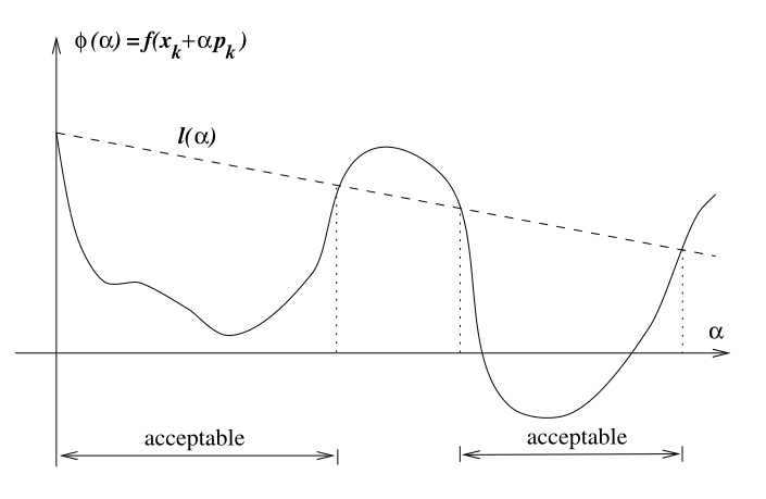
“Approximately” solve this problem to figure out the step length \alpha \min_{\alpha > 0} f(x_k + \alpha p_k)
. . .
We are finding the distance to move ( \alpha) along direction p_k that minimizes our objective f
. . .
Typically, algorithms do not perform the full minimization problem since it is costly
Typical line search algorithms select the step length in two stages
A widely-used method is the Backtracking procedure
. . .
\phi(\alpha) \equiv f(x_k + \alpha p_k) \leq f(x_k) + c\alpha\nabla f_k^T p_k \equiv l(\alpha)
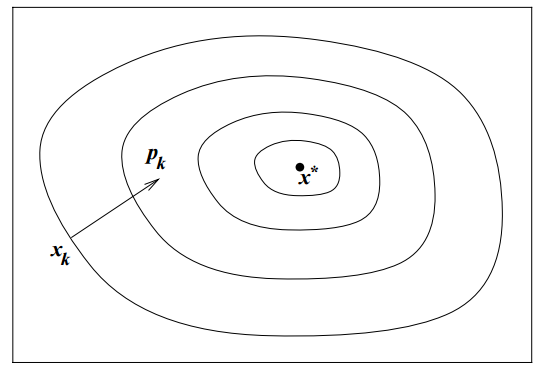
We still haven’t answered, what direction p_k do we decide to move in?
What’s an obvious choice for p_k?
. . .
The direction that yields the steepest descent
. . .
-\nabla f_k is the direction that makes f decrease most rapidly
We can verify this is the direction of steepest descent by referring to Taylor’s theorem
. . .
For any direction p and step length \alpha, we have that
f(x_k + \alpha p) = f(x_k) + \alpha p^T \nabla f_k + \frac{1}{2!}\alpha^2 p^T\nabla^2 f_k p
. . .
The rate of change in f along p at x_k (\alpha = 0) is p^T \, \nabla\,f_k
The the unit vector of quickest descent solves
\min_p p^T\,\nabla\,f_k \,\,\,\,\, \text{subject to: }||p|| = 1
. . .
Re-express the objective as
\min_{\theta,||p||} ||p||\,||\nabla\,f_k||cos\,\theta
where \theta is the angle between p and \nabla\,f_k
. . .
The minimum is attained when cos\,\theta = -1 and p = -\frac{\nabla\,f_k}{||\nabla\,f_k||}, so the direction of steepest descent is simply -\nabla\,f_k
The steepest descent method searches along this direction at every iteration k
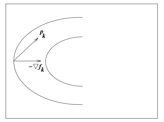
We can always use search directions other than the steepest descent
Any descent direction (i.e. one with angle strictly less than 90^\circ of -\nabla\,f_k) is guaranteed to produce a decrease in f as long as the step size is sufficiently small
But is -\nabla\,f_k always the best search direction?
The most important search direction is not steepest descent but Newton’s direction
. . .
This direction gives rise to the Newton-Raphson Method
Newton’s direction comes out of the second order Taylor series approximation to f(x_k + p)
f(x_k + p) \approx f_k + p^T\,\nabla\,f_k + \frac{1}{2!}\,p^T\,\nabla^2f_k\,p
. . .
We find the Newton direction by selecting the vector p that minimizes f(x_k + p)
. . .
This ends up being
p^N_k = -[\nabla^2 f_k]^{-1}\nabla f_k
The algorithm is pretty much the same as in Newton’s rootfinding method
. . .
This approximation to the function we are trying to solve has error of O(||p||^3), so if p is small, the quadratic approximation is very accurate
. . .
Drawbacks:
Just like in rootfinding, there are several methods to avoid computing derivatives (Hessians, in this case)
Instead of the true Hessian \nabla^2 f(x), these methods use an approximation B_k (to the inverse of the Hessian). Hence, they set direction
d_k = -B_k \nabla f_k
. . .
The optimization method analogous to Broyden’s that also uses the secant condition is the BFGS method
Once again, we will use Optim.jl. We’ll see an example with an easy function, solving it using Steepest Descent, Newton-Raphson, and BFGS
(x_1, x_2) = ax_1^2 + bx_2^2 + cx_1 + dx_2 + ex_1 x_2
We will use parameters a=1, b=4, c=-2, d=-1, e=-3
using Optim, Plots, LinearAlgebra;
a = 1; b = 4; c = -2; d = -1; e = -3;
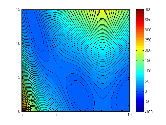
f(x) = a*x[1]^2 + b*x[2]^2 + c*x[1] + d*x[2] + e*x[1]*x[2];Let’s take a look at our function with a contour plot
curve_levels = exp.(0:log(1.2):log(500)) .- 5; # Define manual, log-scale levels for a nicer lookPlots.contour(-5.0:0.1:10.0, -5:0.1:10.0, (x,y)->f([x, y]),
fill = true, levels = curve_levels, size = (400, 300))┌ Warning: GR: highest contour level less than maximal z value is not supported. └ @ Plots ~/.julia/packages/Plots/AE0LB/src/backends/gr.jl:579
Since we will use Newton-Raphson, we should define the gradient and the Hessian of our function
# Gradient
function g!(G, x)
    G[1] = 2a*x[1] + c + e*x[2]
    G[2] = 2b*x[2] + d + e*x[1]
end;

# Hessian
function h!(H, x)
    H[1,1] = 2a
    H[1,2] = e
    H[2,1] = e
    H[2,2] = 2b
end;Let’s check if the Hessian satisfies it being positive semidefinite. One way is to check whether all eigenvalues are positive. In this case, H is constant, so it’s easy to check
H = zeros(2,2);
h!(H, [0 0]);
LinearAlgebra.eigen(H).values
2-element Vector{Float64}:
0.7573593128807148
9.242640687119286Since the gradient is linear, it is also easy to calculate the minimizer analytically. The FOC is just a linear equation
analytic_x_star = [2a e; e 2b]\[-c ;-d]2-element Vector{Float64}:
2.714285714285715
1.142857142857143Let’s solve it with the Steepest (or Gradient) descent method
# Initial guess
x0 = [0.2, 1.6];
res_GD = Optim.optimize(f, g!, x0, GradientDescent(), Optim.Options(x_abstol=1e-3))
* Status: success
* Candidate solution
Final objective value: -3.285714e+00
* Found with
Algorithm: Gradient Descent
* Convergence measures
|x - x'| = 4.55e-04 ≤ 1.0e-03
|x - x'|/|x'| = 1.68e-04 ≰ 0.0e+00
|f(x) - f(x')| = 1.25e-06 ≰ 0.0e+00
|f(x) - f(x')|/|f(x')| = 3.80e-07 ≰ 0.0e+00
|g(x)| = 4.83e-04 ≰ 1.0e-08
* Work counters
Seconds run: 0 (vs limit Inf)
Iterations: 9
f(x) calls: 27
∇f(x) calls: 27Let’s solve it with the Steepest (or Gradient) descent method
res_GD.minimizer2-element Vector{Float64}:
2.7136160576693613
1.142571554006051res_GD.minimum-3.285714084769726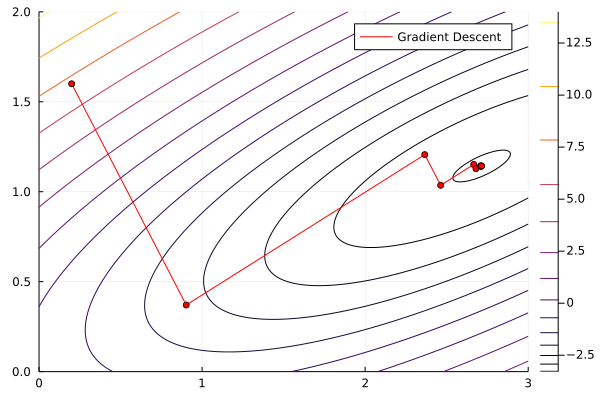
We haven’t really specified a line search method yet
In most cases, Optim.jl will use by default the Hager-Zhang method
. . .
But we can specify other approaches. We need the LineSearches package to do that:
using LineSearches;. . .
Let’s re-run the GradientDescent method using \bar{\alpha}=1 and the backtracking method
Optim.optimize(f, g!, x0,
               GradientDescent(alphaguess = LineSearches.InitialStatic(alpha=1.0),
                               linesearch = BackTracking()),
               Optim.Options(x_abstol=1e-3))
* Status: success
* Candidate solution
Final objective value: -3.285714e+00
* Found with
Algorithm: Gradient Descent
* Convergence measures
|x - x'| = 3.61e-04 ≤ 1.0e-03
|x - x'|/|x'| = 1.33e-04 ≰ 0.0e+00
|f(x) - f(x')| = 8.65e-07 ≰ 0.0e+00
|f(x) - f(x')|/|f(x')| = 2.63e-07 ≰ 0.0e+00
|g(x)| = 6.73e-04 ≰ 1.0e-08
* Work counters
Seconds run: 0 (vs limit Inf)
Iterations: 11
f(x) calls: 18
∇f(x) calls: 12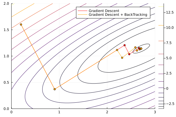
Next, let’s use the Newton-Raphson method with default (omitted) line search parameters
g! and h!, Optim will approximate them numerically for you. You can also specify options to use auto differentiationOptim.optimize(f, g!, h!, x0, Newton()) * Status: success
* Candidate solution
Final objective value: -3.285714e+00
* Found with
Algorithm: Newton's Method
* Convergence measures
|x - x'| = 2.51e+00 ≰ 0.0e+00
|x - x'|/|x'| = 9.26e-01 ≰ 0.0e+00
|f(x) - f(x')| = 1.06e+01 ≰ 0.0e+00
|f(x) - f(x')|/|f(x')| = 3.23e+00 ≰ 0.0e+00
|g(x)| = 4.44e-16 ≤ 1.0e-08
* Work counters
Seconds run: 0 (vs limit Inf)
Iterations: 1
f(x) calls: 4
∇f(x) calls: 4
∇²f(x) calls: 1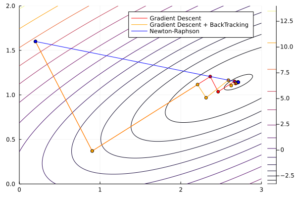
Lastly, let’s use the BFGS method
Optim.optimize(f, x0, BFGS()) * Status: success
* Candidate solution
Final objective value: -3.285714e+00
* Found with
Algorithm: BFGS
* Convergence measures
|x - x'| = 1.81e+00 ≰ 0.0e+00
|x - x'|/|x'| = 6.67e-01 ≰ 0.0e+00
|f(x) - f(x')| = 1.47e+00 ≰ 0.0e+00
|f(x) - f(x')|/|f(x')| = 4.48e-01 ≰ 0.0e+00
|g(x)| = 6.42e-11 ≤ 1.0e-08
* Work counters
Seconds run: 0 (vs limit Inf)
Iterations: 2
f(x) calls: 6
∇f(x) calls: 6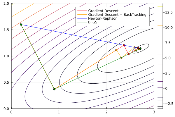
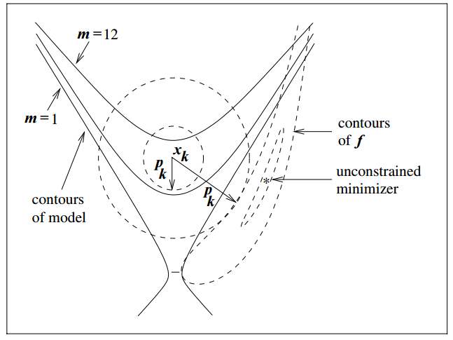
Trust region methods construct an approximating model, m_k whose behavior near the current iterate x_k is close to that of the actual function f
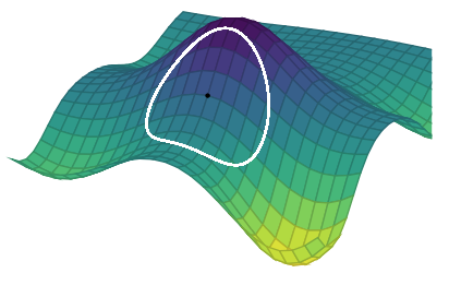
We then search for a minimizer of m_k
Issue: m_k may not represent f well when far away from the current iterate x_k
. . .
Solution: Restrict the search for a minimizer to be within some region of x_k, called a trust region2
Trust region problems can be formulated as
\min_p m_k(x_k + p)
where x_k+p \in \Gamma
. . .
\Delta_k is adjusted every iteration based on how well m_k approximates f_k around current guess x_k
Typically the approximating model m_k is a quadratic function (i.e. a second-order Taylor approximation)
m_k(x_k + p) = f_k + p^T\,\nabla\,f_k + \frac{1}{2!}\,p^T\,B_k\,p
where B_k is the Hessian or an approximation to the Hessian
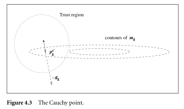
Solving this problem usually involves finding the Cauchy point
From x_k, the Cauchy point can be found in the direction
p^C_k = -\tau_k \frac{\Delta_k}{||\nabla f_k||} \nabla f_k
So it’s kind of a gradient descent ( -\nabla f_k), but with an adjusted step size within the trust region.
The step size depends on the radius \Delta_k and parameter \tau_k
\begin{gather} \tau_k = \begin{cases} 1 & \text{if} \; \nabla f_k^T B_k \nabla f_k \leq 0\\ \min(||\nabla f_k||^3/\Delta_k \nabla f_k^T B_k \nabla f_k, 1) & \text{otherwise} \end{cases} \end{gather}
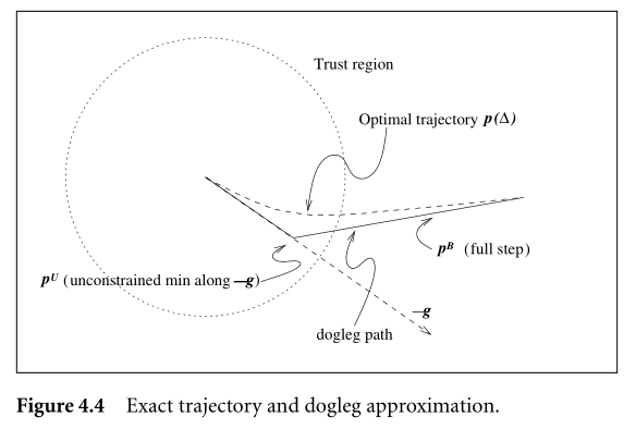
Using default configurations in solvers, you may notice sometimes they use Trust region with dogleg. What is that?
It’s an improvement on the Cauchy point method
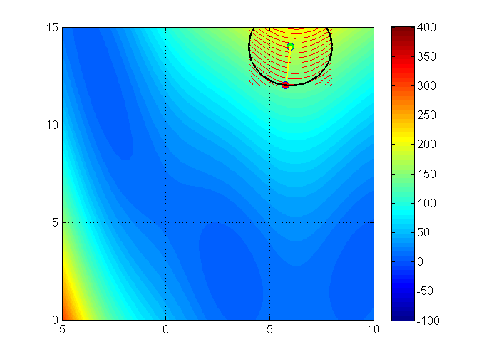
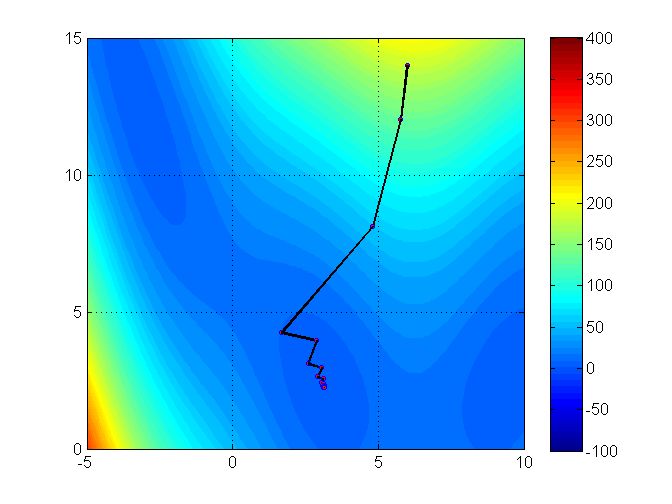
Let’s see an illustration of the trust region method with the Branin function (it has 3 global minimizers)3
min f(x_1, x_2) = (x_2 - 0.129x_1^2 + 1.6 x_1 - 6)^2 + 6.07 \cos(x_1) + 10
Contour plot
Iteration 1
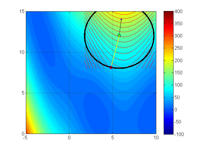
Iteration 2
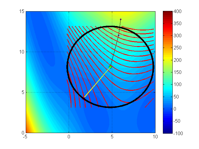
Iteration 3
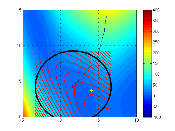
Iteration 4
Iteration 5

Iteration 6
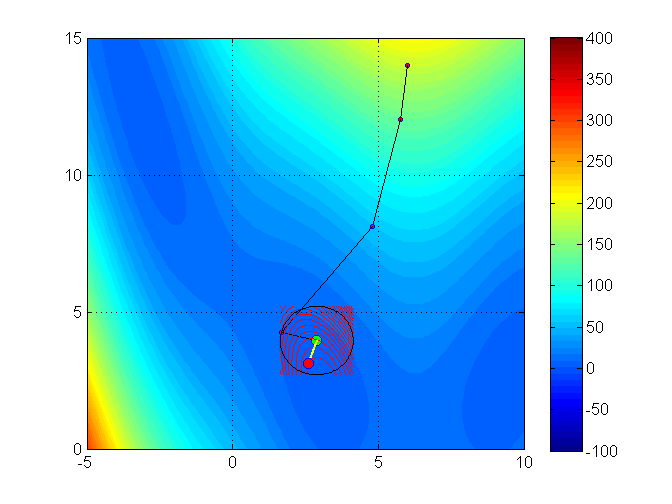
Full trajectory
In Julia, Optim includes a NewtonTrustRegion() solution method. To use it, you can call optimize just like you did with Newton()
Let’s use NewtonTrustRegion to solve the same quadratic function from before4
f(x_1, x_2) = ax_1^2 + bx_2^2 + cx_1 + dx_2 + ex_1 x_2
With parameters a=1, b=4, c=-2, d=-1, e=-3
a = 1; b = 4; c = -2; d = -1; e = -3;
f(x) = a*x[1]^2 + b*x[2]^2 + c*x[1] + d*x[2] + e*x[1]*x[2];
# Complete the arguments of the call
Optim.optimize(<?>, <?>, <?>, <?>, <?>)a = 1; b = 4; c = -2; d = -1; e = -3;
f(x) = a*x[1]^2 + b*x[2]^2 + c*x[1] + d*x[2] + e*x[1]*x[2];
res = Optim.optimize(f, g!, h!, x0, NewtonTrustRegion());
print(res) * Status: success
* Candidate solution
Final objective value: -3.285714e+00
* Found with
Algorithm: Newton's Method (Trust Region)
* Convergence measures
|x - x'| = 1.85e+00 ≰ 0.0e+00
|x - x'|/|x'| = 6.83e-01 ≰ 0.0e+00
|f(x) - f(x')| = 2.15e+00 ≰ 0.0e+00
|f(x) - f(x')|/|f(x')| = 6.54e-01 ≰ 0.0e+00
|g(x)| = 4.44e-16 ≤ 1.0e-08
* Work counters
Seconds run: 0 (vs limit Inf)
Iterations: 2
f(x) calls: 3
∇f(x) calls: 3
∇²f(x) calls: 3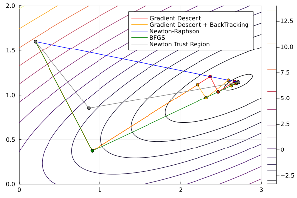
Several other step lenght methods exist. See Nocedal & Wright Ch.3 and Miranda & Fackler Ch 4.4 for more examples.↩︎
We are only going to cover the basic of trust region methods. For details, see Nocedal & Wright (2006), Chapter 4.↩︎
Source for this example: https://arch.library.northwestern.edu/downloads/9z903006b↩︎
*Use default parameters. You can tweak solver parameters later by checking out the documentation https://julianlsolvers.github.io/Optim.jl/stable/#algo/newton_trust_region/↩︎