where \(\theta\) is the angle between \(p\) and \(\nabla\,f_k\)
The minimum is attained when \(cos\,\theta = -1\) and \(p = -\frac{\nabla\,f_k}{||\nabla\,f_k||},\) so the direction of steepest descent is simply \(-\nabla\,f_k\)
Steepest descent method
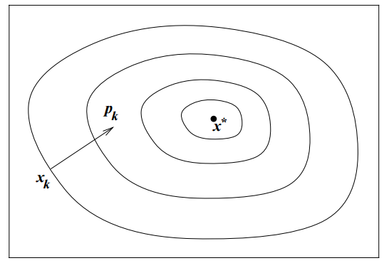
The steepest descent method searches along this direction at every iteration \(k\)
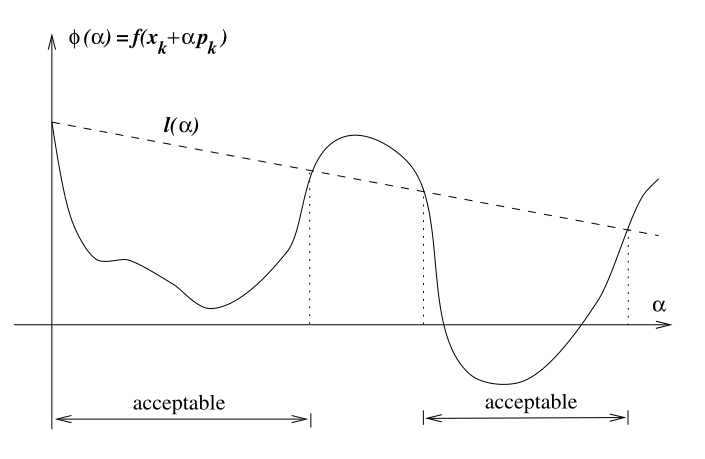
It may select the step length \(\alpha_k\) in several different ways
A benefit of the algorithm is that we only require the gradient of the function, and no Hessian
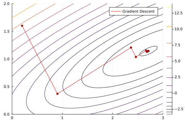
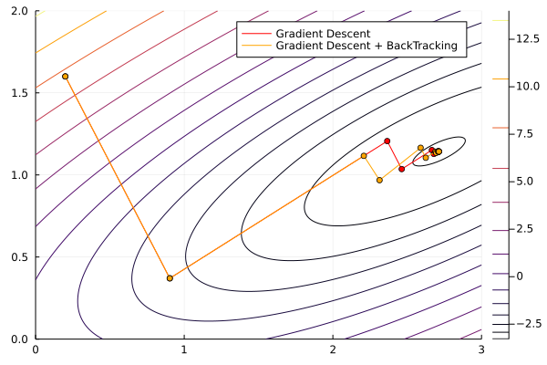
However it can be very slow
Line search: alternative directions
We can always use search directions other than the steepest descent
Any descent direction (i.e. one with angle strictly less than \(90^\circ\) of \(-\nabla\,f_k\)) is guaranteed to produce a decrease in \(f\) as long as the step size is sufficiently small
But is \(-\nabla\,f_k\) always the best search direction?
Newton-Raphson method
The most important search direction is not steepest descent but Newton’s direction
This direction gives rise to the Newton-Raphson Method
This method is basically just using Newton’s method to find the root of the gradient of the objective function
Newton-Raphson method
Newton’s direction comes out of the second order Taylor series approximation to \(f(x_k + p)\)
We find the Newton direction by selecting the vector \(p\) that minimizes \(f(x_k + p)\)
This ends up being
\[
p^N_k = -[\nabla^2 f_k]^{-1}\nabla f_k
\]
Newton-Raphson method
The algorithm is pretty much the same as in Newton’s rootfinding method
Start with an initial guess \(x_0\)
Repeat until convergence
\(x_{k+1} \leftarrow x_{k} - \alpha_k [\nabla^2 f_k]^{-1}\nabla f_k\), where \(\alpha_k\) comes from a step length selection algorithm
Terminate with \(x^* = x_{k}\)
Most packages just use \(\alpha=1\) (i.e., Newton’s method step). But you can usually change this parameter if you have convergence issues
Newton-Raphson method
This approximation to the function we are trying to solve has error of \(O(||p||^3)\), so if \(p\) is small, the quadratic approximation is very accurate
Drawbacks:
The Newton direction is only guaranteed to decrease the objective function if \(\nabla^2 f_k\) is positive definite
It requires explicit computation of the Hessian, \(\nabla^2 f(x)\)
But quasi-Newton solvers also exist
Quasi-Newton methods
Just like in rootfinding, there are several methods to avoid computing derivatives (Hessians, in this case)
Instead of the true Hessian \(\nabla^2 f(x)\), these methods use an approximation \(B_k\) (to the inverse of the Hessian). Hence, they set direction
\[
d_k = -B_k \nabla f_k
\]
The optimization method analogous to Broyden’s that also uses the secant condition is the BFGS method
Named after its inventors, Broyden, Fletcher, Goldfarb, Shanno
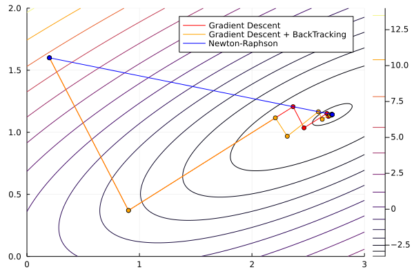
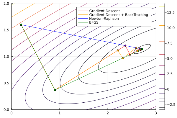
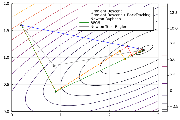
Linear search methods in practice
Once again, we will use Optim.jl. We’ll see an example with an easy function, solving it using Steepest Descent, Newton-Raphson, and BFGS
Let’s check if the Hessian satisfies it being positive semidefinite. One way is to check whether all eigenvalues are positive. In this case, \(H\) is constant, so it’s easy to check
H =zeros(2,2);h!(H, [00]);LinearAlgebra.eigen(H).values
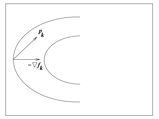
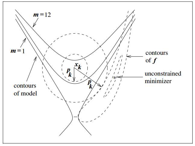
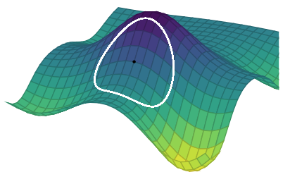
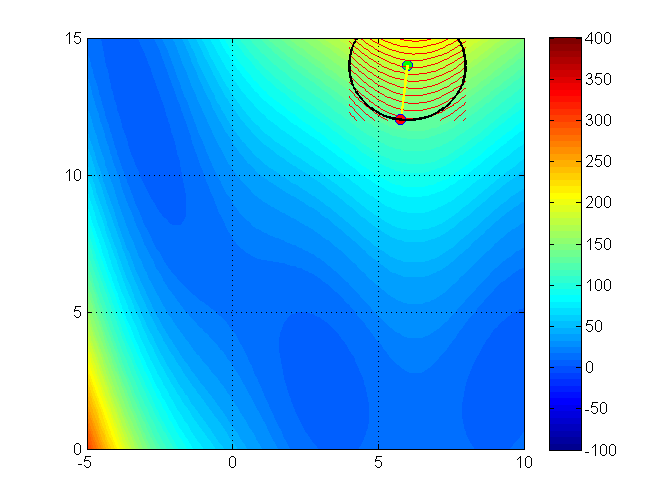
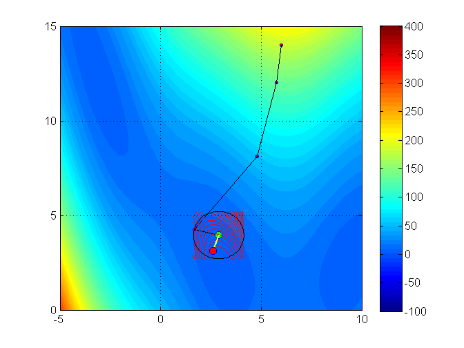
Trust region methods construct an approximating model, \(m_k\) whose behavior near the current iterate \(x_k\) is close to that of the actual function \(f\)
We then search for a minimizer of \(m_k\)
Trust region methods
Issue:\(m_k\) may not represent \(f\) well when far away from the current iterate \(x_k\)
Solution: Restrict the search for a minimizer to be within some region of \(x_k\), called a trust region1
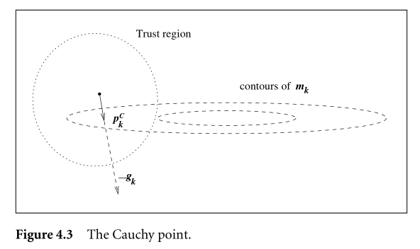
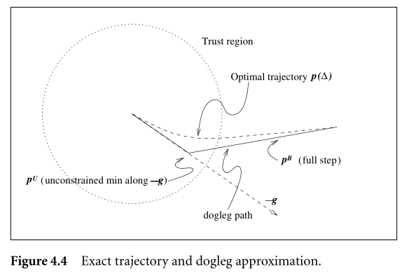
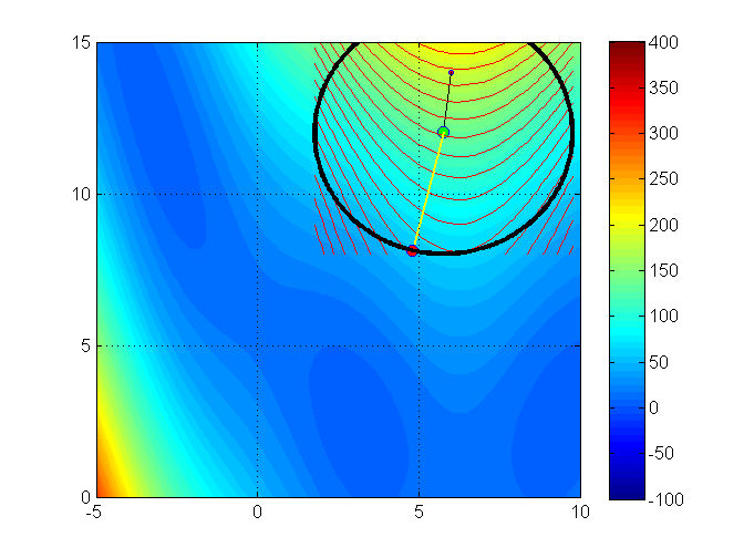
Trust region methods
Trust region problems can be formulated as
\[
\min_p m_k(x_k + p)
\]
where \(x_k+p \in \Gamma\)
\(\Gamma\) is a ball defined by \(||p||_2 \leq \Delta_k\)
\(\Delta_k\) is called the trust region radius
\(\Delta_k\) is adjusted every iteration based on how well \(m_k\) approximates \(f_k\) around current guess \(x_k\)
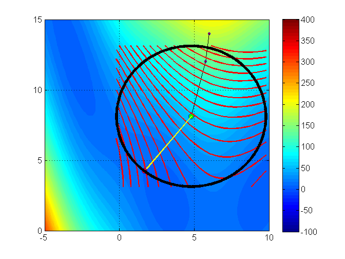
Trust region methods
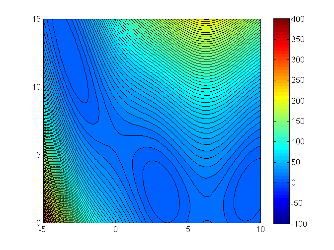
Typically the approximating model \(m_k\) is a quadratic function (i.e. a second-order Taylor approximation)
a =1; b =4; c =-2; d =-1; e=-3;f(x) = a*x[1]^2+ b*x[2]^2+ c*x[1] + d*x[2] +e*x[1]*x[2];# Complete the arguments of the callOptim.optimize(<?>, <?>, <?>, <?>, <?>)
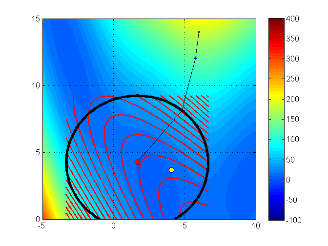
Trust region methods in Julia
a =1; b =4; c =-2; d =-1; e=-3;f(x) = a*x[1]^2+ b*x[2]^2+ c*x[1] + d*x[2] +e*x[1]*x[2];res = Optim.optimize(f, g!, h!, x0, NewtonTrustRegion());print(res)