ACE 592 - Lecture 1.3

An introduction to programming with Julia

Author

Affiliation

Diego S. Cardoso

University of Illinois Urbana-Champaign

0.1 Course Roadmap

1. Introduction to Scientific Computing
   1. Motivation
   2. Best practices
   3. Intro to programming
2. Fundamentals of numerical methods
3. Systems of equations
4. Optimization
5. Function approximation
6. Structural estimation

0.2 Agenda

• Today we start a crash course on programming using Julia
• We will cover the main features to get you started…
• Of course, we’ll be just scratching the surface. You’ll learn a lot more as we go

. . .

• Unless you told me you are using a different language, by now you hopefully have installed
  • Julia
  • Visual Studio Code with Julia extension

0.3 Relevant sources for this lecture

• Software Carpentry
• QuantEcon
• Lecture notes for Grant McDermott’s Data Science for Economists (Oregon) and Ivan Rudik’s Dynamic Optimization (Cornell)
• Julia documentation

0.4 Why learn Julia?

Reason 1: It is easy to learn and use

Julia is a high-level language

• Low-level = you write instructions are closer to what the hardware understands (Assembly, C++, Fortran)
  • These are usually the fastest because there is little to translate (what a compiler does) and you can optimize your code depending on your hardware
• High-level means you write in closer to human language (Julia, R, Python)
  • The compiler has to do a lot more work to translate your instructions

0.5 Why learn Julia?

Reason 2: Julia delivers C++ and Fortran speed

Sounds like magic, but it’s just a clever combination of design choices targeting numerical methods

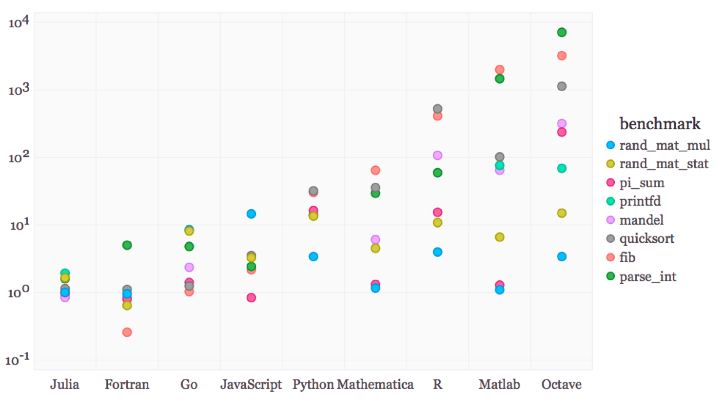
In this graph, time to execute in C++ is 1

0.6 Why learn Julia?

Reason 3: Julia is free, open-source, and popular

• You don’t need expensive licenses to use (unlike Matlab)
• The people who want to use or verify what you did also don’t have to pay
• There is a large and active community of users and developers
  • So it’s easy to get help and new packages

0.7 Tools for programming in Julia

There are 2 Integrated Development Environments (IDEs) I generally recommend

1. Visual Studio (VS) code
2. Jupyter Lab notebooks

. . .

In this course, we will only program plain .jl files, so I highly recommend you get familiarized with VS code

. . .

• At the end of this unit, we will talk about using AI tools to help you learn to code and become a more productive programmer

0.8 Intro to programming

Programming \equiv writing a set of instructions

• There are hard rules you can’t break if you want your code to work

. . .

• There are elements of style (e.g. Strunk and White) that make your code easier to read, modify, and maintain

. . .

• There are elements that make your code more efficient
  • Using less time or space (memory)

0.9 Intro to programming

If you will be doing computational work, there are:

1. Language-independent coding basics you should know
   • Arrays are stored in memory in particular ways
2. Language-independent best practices you should use
   • Indent to convey program structure, naming conventions
3. Language-dependent idiosyncracies that matter for function, speed, etc
   • Vectorizing, memory management

0.10 Intro to programming

Learning these early will:

1. Make coding a lot easier

. . .

2. Reduce total programmer time

. . .

3. Reduce total computer time

. . .

4. Make your code understandable by someone else or your future self

. . .

5. Make your code flexible

0.11 A broad view of programming

Your goal is to make a program

A program is made of different components and sub-components

. . .

The most basic component is a statement, more commonly called a line of code

0.12 A broad view of programming

Here is an example of a pseudoprogram:

deck = ["4 of hearts", "King of clubs", "Ace of spades"]
shuffled_deck = shuffle(deck)
first_card = shuffled_deck[1]
println("The first drawn card was " * shuffled_deck ".")

This program is very simple:

. . .

1. Create a deck of cards

0.13 A broad view of programming

Here is an example of a pseudoprogram:

deck = ["4 of hearts", "King of clubs", "Ace of spades"]
shuffled_deck = shuffle(deck)
first_card = shuffled_deck[1]
println("The first drawn card was " * shuffled_deck ".")

This program is very simple:

1. Create a deck of cards

2. Shuffle the deck

0.14 A broad view of programming

Here is an example of a pseudoprogram:

deck = ["4 of hearts", "King of clubs", "Ace of spades"]
shuffled_deck = shuffle(deck)
first_card = shuffled_deck[1]
println("The first drawn card was " * shuffled_deck ".")

This program is very simple:

1. Create a deck of cards

2. Shuffle the deck

3. Draw the top card

0.15 A broad view of programming

Here is an example of a pseudoprogram:

deck = ["4 of hearts", "King of clubs", "Ace of spades"]
shuffled_deck = shuffle(deck)
first_card = shuffled_deck[1]
println("The first drawn card was " * shuffled_deck ".")

This program is very simple:

1. Create a deck of cards

2. Shuffle the deck

3. Draw the top card

4. Print it

0.16 A broad view of programming

deck = ["4 of hearts", "King of clubs", "Ace of spades"]
shuffled_deck = shuffle(deck)
first_card = shuffled_deck[1]
println("The first drawn card was " * shuffled_deck ".")

What are the parentheses and why are they different from square brackets?

How does shuffle work?

What’s println?

It’s important to know that a good program has understandable code

0.17 Julia specifics

We will discuss coding in the context of Julia but a lot of this ports to Python, MATLAB, etc¹

We will review

1. Types
2. Functions
3. Iterating
4. Broadcasting/vectorization

. . .

And some slightly more advanced aspects to help you debug

5. Scope
6. Multiple dispatch

1 1. Types

1.1 Types: boolean

All languages have some kind of variable types like integers or arrays

. . .

The first type you will often use is a boolean (Bool) variable that takes on a value of true or false:

x = true

true

typeof(x)

Bool

1.2 Types: boolean

We can save the boolean value of actual statements in variables this way:

@show y = 1 > 2

y = 1 > 2 = false

false

• @show is a Julia macro for showing the operation.
• You can think of a macro as a shortcut name that calls a bunch of other things to run

1.3 Quick detour: logical operators

Logical operators work like you’d think

== (equal equal) tests for equality

1 == 1

true

. . .

!= (exclaimation point equal) tests for inequality

2 != 2

false

1.4 Quick detour: logical operators

You can also test for approximate equality with \approx (type \approx<TAB>)

1.00000001 ≈ 1

true

• We will see why this can be super useful in the next unit

. . .

Now back to types

1.5 Types: numbers

Two other data types you will use frequently are integers

typeof(1)

Int64

. . .

and floating point numbers

typeof(1.0)

Float64

• 64 means 64 bits of storage for the number, which is probably the default on your machine

1.6 Types: numbers

You can always instantiate alternative floating point number types

converted_int = convert(Float32, 1.0);
typeof(converted_int)

Float32

1.7 Types: numbers

Math works like you would expect:

a = 2

2

b = 1.0

1.0

a * b

2.0

. . .

a^2

4

1.8 Types: numbers

2a - 4b

0.0

. . .

@show 4a + 3b^2

4a + 3 * b ^ 2 = 11.0

11.0

. . .

In Julia, you dont need * in between numeric literals (numbers) and variables

• But I advise you use the explicit notation anyway to avoid bugs

1.9 Types: strings

Strings store sequences of characters

You implement them with double quotations:

x = "Hello World!";
typeof(x)

String

. . .

• Note that ; is used to suppress output for that line of code
• Unlike some other languages, in Julia you don’t need to add ; after every command

1.10 Types: strings

It’s easy to work with strings. Use $ to interpolate a variable/expression

x = 10; y = 20; println("x + y =  $(x+y).")

x + y =  30.

. . .

Use * to concatenate strings

a = "Aww"; b = "Yeah!!!"; println(a * " " * b)

Aww Yeah!!!

. . .

You probably won’t use strings too often unless you’re working with text data or printing output.

. . .

• Note that ; can also be used to type multiple commands in the same line. I’m doing it make all fit in one slide, but you should avoid it

1.11 Types: containers

Containers are types that store collections of data

. . .

The most basic container is the Array which is denoted by square brackets

. . .

a1 = [1 2; 3 4]; typeof(a1)

Matrix{Int64} (alias for Array{Int64, 2})

. . .

Arrays are mutable, which means you can change their values

. . .

a1[1,1] = 5; a1

2×2 Matrix{Int64}:
 5  2
 3  4

You reference elements in a container with square brackets

1.12 Types: containers

An alternative to the Array is the Tuple, which is denoted by parentheses

. . .

a2 = (1, 2, 3, 4); typeof(a2)

NTuple{4, Int64}

a2 is a Tuple of 4 Int64s. Tuples have no dimension

1.13 Types: containers

Tuples are immutable which means you can’t change their values

try
  a2[1] = 5;
catch
  println("Error, can't change value of a tuple.")
end

Error, can't change value of a tuple.

1.14 Types: containers

Tuples don’t need parentheses (but it’s probably best practice for clarity)

a3 = 5, 6; typeof(a3)

Tuple{Int64, Int64}

1.15 Types: containers

Tuples can be unpacked

. . .

a3_x, a3_y = a3;
a3_x

5

a3_y

6

. . .

This is basically how functions return multiple outputs when you call them!

1.16 Types: containers

But an alternative and more efficient container is the NamedTuple

nt = (x = 10, y = 11); typeof(nt)

@NamedTuple{x::Int64, y::Int64}

nt.x

10

nt.y

11

Another way of accessing x and y inside the NamedTuple is

nt[:x]

10

nt[:y];

1.17 Types: containers

A Dictionary is the last main container type

• They are like arrays but are indexed by keys (names) instead of numbers

. . .

d1 = Dict("class" => "ACE592", "grade" => 97);
typeof(d1)

Dict{String, Any}

. . .

d1 is a dictionary where the key are strings and the values are any kind of type

1.18 Types: containers

Reference specific values you want in the dictionary by referencing the key

. . .

d1["class"]

"ACE592"

d1["grade"]

97

1.19 Types: containers

If you just want all the keys or all the values, you can use these base functions

keys_d1 = keys(d1)

KeySet for a Dict{String, Any} with 2 entries. Keys:
  "class"
  "grade"

values_d1 = values(d1)

ValueIterator for a Dict{String, Any} with 2 entries. Values:
  "ACE592"
  97

1.20 Creating new types

We can actually create new composite types using struct

. . .

struct FoobarNoType # This will be immutable by default
  a
  b
  c
end

This creates a new type called FoobarNoType

1.21 Creating new types

We can generate a variable of type FoobarNoType using its constructor which will have the same name

. . .

newfoo = FoobarNoType(1.3, 2, "plzzz");
typeof(newfoo)

FoobarNoType

newfoo.a

1.3

1.22 Creating new types

Custom types are a handy and elegant way of organizing your program

• You can define a type ModelParameters to contain all your model parameters

• Each variable you instantiate represents a single scenario

• Then, instead of having a function call

RunMyModel(param1, param2, param3, param4, param5);

• You call

RunMyModel(modelParameters);

1.23 Creating new types

You should always declare types for the fields of a new composite type

. . .

You can declare types with the double colon

struct FoobarType # This will be immutable by default
  a::Float64
  b::Int
  c::String
end

1.24 Creating new types

newfoo_typed = FoobarType(1.3, 2, "plzzz");
typeof(newfoo_typed)

FoobarType

newfoo.a

1.3

This lets the compiler generate efficient code because it knows the types of the fields when you construct a FoobarType

2 2. Functions

2.1 Functions: why?

Functions are an essential part of programming. But why use functions?

1. To avoid duplicating code
   • If you have the same set of instructions repeated in multiple parts of your code, whenever you need to change something, you have to search through the code and change in many places. This is prone to bugs!
   • Rule of thumb: if you are using same (or a very similar) block of the instructions more than twice, turn that block into a function

2.2 Functions: why?

2. To make our program more efficient
   • Julia optimizes functions in the background, but not code outside functions (more on that soon)

. . .

3. To make our code easier to read

• Functions can give meaninful names to a block of code that does a specific tasks
• Also, it can generalize the operation, letting that block take in different values

2.3 Functions: defining them

Creating functions in Julia is easy

function my_function(argument_1, argument_2)
  # Do something here
end;
typeof(my_function)

typeof(my_function) (singleton type of function my_function, subtype of Function)

. . .

You can also define functions with no arguments. This can be, for example, for some calculation that will print results or save them in a file or manipulate objects somewhere in memory

function my_other_function()
  # Add something here
end;

2.4 Functions: defining them

If you have a simple mathematical function, like F(x) = \sin(x^2), you can use shorthand notation like this

F(x) = sin(x^2)

F (generic function with 1 method)

. . .

This is the same as

function F(x)
  sin(x^2)
end

F (generic function with 1 method)

2.5 Functions: return values

function F(x)
  sin(x^2)
end

By default, a function will return the last value it evaluated

F(1)

0.8414709848078965

2.6 Functions: return values

But it’s a good practice to make the return value explicit

function F(x)
  result = sin(x^2)
  return result
end;
F(1)

0.8414709848078965

2.7 Functions: return values

Specifying a return is a must if you want to return multiple values. You can do that with tuples!

function flip_coordinates(lat, long)
  flipped_lat = -lat
  flipped_long = -long
  return flipped_lat, flipped_long
end;
x1, x2 = flip_coordinates(45, -60)

(-45, 60)

2.8 Tangent: JIT

• Just-in-time compilation (JIT) is one of the tricks Julia does to make things run faster
  • It translates your code to processor language the first time you run it and uses the translated version every time you call it again
  • When we run the function for the first time, it may take longer because of this compilation step
  • When we run it again, it will be much faster
• This is one of the reasons why putting your code inside functions is important: Julia can optimize functions better than code outside functions

3 3. Iteration

3.1 Iterating

As in other languages we have loops at our disposal:

for loops iterate over containers

for count in 1:10
  random_number = rand()
  if random_number > 0.2
    println("We drew a $random_number.")
  end
end

We drew a 0.9713252699989239.
We drew a 0.8935560266818744.
We drew a 0.7167227993052901.
We drew a 0.2182980537935365.
We drew a 0.23761909239132128.
We drew a 0.8068367563280319.
We drew a 0.45899540819101947.
We drew a 0.35568275048345566.
We drew a 0.8399740473590757.

3.2 Iterating

while loops iterate until a logical expression is false

x = 1;
while x < 50
  x = x * 2
  println("After doubling, x is now equal to $x.")
end

After doubling, x is now equal to 2.
After doubling, x is now equal to 4.
After doubling, x is now equal to 8.
After doubling, x is now equal to 16.
After doubling, x is now equal to 32.
After doubling, x is now equal to 64.

3.3 Iterating

An Iterable is something you can loop over, like arrays

. . .

actions = ["codes well", "skips class"];
for action in actions
    println("Charlie $action")
end

Charlie codes well
Charlie skips class

3.4 Iterating

The type Iterator is a particularly convenient subset of Iterables

. . .

These include things like the dictionary keys:

for key in keys(d1)
  println(d1[key])
end

ACE592
97

3.5 Iterating

Iterating on Iterators is more memory efficient than iterating on arrays

. . .

Here’s a very simple example. The top function iterates on an Array, the bottom function iterates on an Iterator:

. . .

function show_array_speed()
  m = 1
  for i = [1, 2, 3, 4, 5, 6]
    m = m*i
  end
end;

function show_iterator_speed()
  m = 1
  for i = 1:6
    m = m*i
  end
end;

3.6 Iterating

using BenchmarkTools
@btime show_array_speed()
@btime show_iterator_speed()

  2.350 ns (0 allocations: 0 bytes)
  1.709 ns (0 allocations: 0 bytes)

The Iterator approach is faster and allocates no memory

• @btime is a macro from package BenchmarkTools that shows you the elasped time and memory allocation

3.7 Neat looping

A nice thing about Julia: your loops can be much neater because you don’t need to index when you just want the container elements

. . .

f(x) = x^2;
x_values = 0:20:100;
for x in x_values
  println(f(x))
end

0
400
1600
3600
6400
10000

3.8 Neat looping

This loop directly assigns the elements of x_values to x instead of having to do something clumsy like x_values[i]

. . .

0:20:100 creates something called a StepRange (a type of Iterator) which starts at 0, steps up by 20 and ends at 100

3.9 Neat looping

You can also pull out an index and the element value by enumerating

f(x) = x^2;
x_values = 0:20:100;
for (index, x) in enumerate(x_values)
  println("f(x) at value $index is $(f(x)).")
end

f(x) at value 1 is 0.
f(x) at value 2 is 400.
f(x) at value 3 is 1600.
f(x) at value 4 is 3600.
f(x) at value 5 is 6400.
f(x) at value 6 is 10000.

enumerate basically assigns an index vector

3.10 Neat looping

Nested loops can also be made very neatly

. . .

for x in 1:3, y in 3:-1:1
  println("$x minus $y is $(x-y)")
end

1 minus 3 is -2
1 minus 2 is -1
1 minus 1 is 0
2 minus 3 is -1
2 minus 2 is 0
2 minus 1 is 1
3 minus 3 is 0
3 minus 2 is 1
3 minus 1 is 2

The first loop is the outer loop, the second loop is the inner loop

3.11 Neat looping

But the “traditional” way of nesting loops also works

• Just remember to include an end for each for nest

for x in 1:3
  for y in 3:-1:1
    println("$x minus $y is $(x-y)")
  end
end

1 minus 3 is -2
1 minus 2 is -1
1 minus 1 is 0
2 minus 3 is -1
2 minus 2 is 0
2 minus 1 is 1
3 minus 3 is 0
3 minus 2 is 1
3 minus 1 is 2

3.12 Comprehensions

Comprehensions are an elegant way to use iterables that makes your code cleaner and more compact

. . .

squared = [y^2 for y in 1:2:11]

6-element Vector{Int64}:
   1
   9
  25
  49
  81
 121

This created a 1-dimension Array using one line

3.13 Comprehensions

We can also use nested loops for comprehensions

. . .

squared_2 = [(y+z)^2 for y in 1:2:11, z in 1:6]

6×6 Matrix{Int64}:
   4    9   16   25   36   49
  16   25   36   49   64   81
  36   49   64   81  100  121
  64   81  100  121  144  169
 100  121  144  169  196  225
 144  169  196  225  256  289

This created a 2-dimensional Array

. . .

• Use this (and the compact nested loop) sparingly since it’s hard to read and understand

4 4. Broadcating/Vectorization

4.1 Vectorization

Iterated operations element by element is usually an inefficient approach

Another way is to do operations over an entire array. This is called vectorization

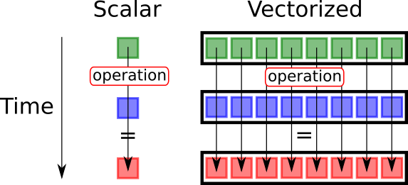
• It’s faster because your processor can do some operations over multiple values with one instruction

4.2 Dot syntax: broadcasting/vectorization

Vectorizing operations is easy in Julia: just use dot syntax (like in MATLAB)

. . .

g(x) = x^2;
squared_2 = g.(1:2:11)

6-element Vector{Int64}:
   1
   9
  25
  49
  81
 121

. . .

This is actually called broadcasting in Julia

4.3 Dot syntax: math intuition

There is a mathematical intuition to make a distinction

• g(x) = x^2 is a function \mathbb{R} \rightarrow \mathbb{R}, i.e., mapping a scalar to a scalar

. . .

• But if z is, say, a 6 \times 1 vector: z \in \mathbb{R}^6, it’s unclear what g(z) is
  • What does the square of a 6 \times 1 vector even mean? Is it the square of each element? Is it a dot product with the vector itself? Something else?

. . .

• When you use the dot syntax g.(1:2:11), you are telling Julia: apply function g to each element in vector [1, 3, 5, 7, 9, 11]
  • If we needed a function to do something else with the whole vector, we need to write a different function for that

4.4 Dot syntax: we must pay attention to definitions!

• Julia will generally be picky about this: if you call a function that is defined for a scalar and give it a vector, you will get an error message
  • This strictness (called “strong typed language”) is actually one of the reasons it gets so fast: it doesn’t need to spend time figuring out what kind of variable you give to it

try
  g(1:2:11)
catch e
  println(e)
end

MethodError(^, (1:2:11, 2), 0x0000000000009825)

. . .

• The try/catch block let’s you handle error messages within your program
  • If anything fails, you can program ways to handle errors
  • We won’t be using it in the course; it’s here just because I have to handle it this way to generate slides. If you run this code, Julia REPL will give you a more informative error message

5 5. Scope

5.1 Scope

The scope of a variable name determines when it is valid to refer to that variable

• E.g.: if you create a variable inside a function, can you reference that variable outside the function?
• You can think of scope as different contexts within your program

. . .

The two basic scopes are local and global

. . .

Scope can be a frustrating concept to grasp at first. But understanding how scopes work can save you a lot of debugging time

. . .

Let’s walk through some simple examples to see how it works

5.2 Scope

First, functions have their own local scope

. . .

ff(xx) = xx^2;
yy = 5;
ff(yy)

25

xx isn’t bound to any values outside the function ff

• It is only used inside the function

5.3 Scope

Locally scoped functions allow us to do things like:

xx = 10;
fff(xx) = xx^2;
fff(5)

25

. . .

Although xx was declared equal to 10 outside the function, the function still evaluated xx within its own scope at 5 (the value passed as argument)

5.4 Scope

But this type of scoping also has (initially) counterintuitive results like:

zz = 0;
function do_some_iteration()
  for ii = 1:10
    zz = ii
  end
end
do_some_iteration()
println("zz = $zz")

zz = 0

. . .

What happened?

5.5 Scope

What happened?

The zz outside the for loop has a different scope: it’s in the global scope

. . .

The global scope is the outermost scope, outside all functions

. . .

The zz inside the function has a scope local to the loop

. . .

Since the outside zz has global scope, the locally scoped variables in the loop can’t change it

5.6 Scope

But hold on. If try the same loop outside a function, it will actually return 10, not 0. ^{*}

zz = 0;
for ii = 1:10
  zz = ii
end
println("zz = $zz")

zz = 10

. . .

That’s because this for loop sits in global scope

• It can get more complicated than that because there are soft and hard local scopes… but we don’t need to dwell on that
• The documentation has the details about the scope of variables

5.7 Scope

Generally, you want to avoid global scope because it can cause conflicts, slowness, etc. But you can use global to force it if you want something to have global scope

• This is almost always a bad practice, though!

zz = 0;
function do_some_iteration()
  for ii = 1:10
    global zz = ii
  end
end
do_some_iteration()
println("zz = $zz")

zz = 10

5.8 Scope

Local scope kicks in whenever you are defining variables inside a function

Global variables inside a local scope are inherited for reading, not writing

x, y = 1, 2;
function foo()
  x = 2        # assignment introduces a new local
  return x + y # y refers to the global
end;
foo()
x

1

5.9 Scope

We can fix looping issues with global scope by using a wrapper function that doesn’t do anything but change the parent scope so it is not global

zzz = 1;
function wrapper()
  zzz = 0;
  for iii = 1:10
    zzz = iii
  end
  println("zzz = $zzz")
end
wrapper()

zzz = 10

6 6. Multiple dispatch

6.1 Multiple dispatch

Julia lets you define multiple functions with the same name but different types of input variables

This is useful because some operations have different steps depending on the context. For example

• Multiplication (*) can work on scalars, vectors, matrices, and more complex types
  • By allowing different instructions depending on what type of variable is given, Julia makes it easier for user to use functions consistently

. . .

• But if you try to call a function with types of input variables it doesn’t know how to handle, it will throw an error
  • This is usually the most common error you will encounter while learning Julia

6.2 Multiple dispatch

/ has MANY different methods for division depending on the input types! Each of these is a function specialized function that treats the inputs differently

length(methods(/))

144

methods(/)[1:4]

4-element Vector{Method}:

• /(::Missing, ::Missing) in Base at missing.jl:122
• /(::Missing, ::Number) in Base at missing.jl:123
• /(x::BigInt, y::BigInt) in Base.GMP at gmp.jl:517
• /(x::BigInt, y::Union{Int16, Int32, Int64, Int8, UInt16, UInt32, UInt64, UInt8}) in Base.GMP at gmp.jl:566

7 General programming advice

7.1 Some concluding words on programming

There is really only one way to effectively get better at programming: PRACTICE

. . .

Yes, reading can help, especially by making you aware of tools and resources. But it’s no substitute for actually solving problems with the computer

7.2 Some concluding words on programming

How to get started with your practice?

My suggestion of an intuitive way: practice writing programs to solve problems you would know how to solve by hand

. . .

• The computer follows a strict logic that very often is different from yours
• Learning how to tell the computer to follow instructions and get to a destination you already know is a great way of learning

. . .

My personal favorite: Project Euler

7.3 Some concluding words on programming

Project Euler is a series of challenging mathematical/computer programming problems that will require more than just mathematical insights to solve. Although mathematics will help you arrive at elegant and efficient methods, the use of a computer and programming skills will be required to solve most problems.

. . .

Example of problems 1. If we list all the natural numbers below 10 that are multiples of 3 or 5, we get 3, 5, 6 and 9. The sum of these multiples is 23. Find the sum of all the multiples of 3 or 5 below 1000. . . .

2. The prime factors of 13195 are 5, 7, 13 and 29. What is the largest prime factor of the number 600851475143 ?

. . .

You can type in your answer and it will tell you if it’s correct

7.4 Some concluding words on programming

More on coding practices and efficiency:

• See JuliaPraxis for best practices for naming, spacing, comments, etc

• See more Performance tips from Julia Documentation

7.5 What about ChatGPT, Claude, and other LLMs?

• You are lucky! You’re among the first cohorts learning to program with an available AI language model that is advanced enough to understand, explain, and generate code

. . .

• Currently, one of the best available services for that is called GitHub Copilot. It’s paid, but you can get it for free with an .edu email

But hold on. Don’t use this powerful resource without careful consideration

7.6 What about ChatGPT, Claude, and other LLMs?

But hold on. Don’t use this powerful resource without careful consideration

• This must be a complement, not a substitute for your programming skills

Why?

. . .

• For especialized scientific use, AI often produces buggy, incomplete, or outright incorrect code
  • Before you use it accurately, you need to be familiar enough with programming logic and the language you are using to know when things are wrong
• These tools are improving fast, but they will always be imperfect
  • There is an inherent limitation in translating ambiguous (natural) languages to non-ambiguous (formal) languages
• Treat it like a very smart intern who can do well-defined tasks very quickly
  • But, to correctly supervise an intern, you need to know the job well yourself!

7.7 Advice on AI coding assistants

Here is my personal advice to you focusing on your the medium/long-term career as a researcher

1. Do not use AI assistants to generate code you still cannot write and understand

• There’s too big of a risk of producing incorrect code
• It will place a low cap on your logical thinking for computational methods
• Once you advance and become familiar with programming structures, you can start relying in AI to speed up your coding
  • For this course, coding assignments are relatively short, so I expect you to know what every line of code you write does

7.8 Advice on AI coding assistants

Here is my personal advice to you focusing on your the medium/long-term career as a researcher

2. Use AI assistants to explain code to you or generate examples

• Throughout the semester, you will see many examples of algorithms
• AI can offer tremendous help explaining the inner workings of algorithms

. . .

3. If you are a good programmer in one language, AI tools can also help you translate code

• Even in that case, I’d still recommend you start using it to explain code in the “new” language rather than simply generate code for you

Footnotes

1. See https://cheatsheets.quantecon.org