---
title: "Session 6 - Spatial Data"
subtitle: "[R for Data Analysis](https://github.com/worldbank)"
author: "DIME Analytics"
date: "The World Bank -- DIME | [WB Github](https://github.com/worldbank)
April 2025"
output:
xaringan::moon_reader:
css: ["libs/remark-css/default.css",
"libs/remark-css/metropolis.css",
"libs/remark-css/metropolis-fonts.css",
"libs/remark-css/custom.css"]
lib_dir: libs
nature:
ratio: "16:9"
highlightStyle: github
highlightLines: true
countIncrementalSlides: false
---
```{r setup, include=FALSE}
options(htmltools.dir.version = FALSE)
library(knitr)
opts_chunk$set(
fig.align="center",
fig.height=4, #fig.width=6,
# out.width="748px", #out.length="520.75px",
dpi=300, #fig.path='Figs/',
cache=T#, echo=F, warning=F, message=F
)
library(hrbrthemes)
library(fontawesome)
library(xaringanExtra)
library(countdown)
xaringanExtra::use_panelset()
xaringanExtra::use_editable()
xaringanExtra::use_clipboard()
xaringanExtra::use_logo(
image_url = "img/lightbulb.png",
exclude_class = c("inverse", "hide_logo"),
width = "50px"
)
htmltools::tagList(
xaringanExtra::use_clipboard(
button_text = "",
success_text = "",
error_text = ""
),
rmarkdown::html_dependency_font_awesome()
)
```
# Table of contents
.large[
1. Overview of GIS concepts
2. Load and explore polygons, polylines, and points
3. Static maps
4. Interactive maps
5. Spatial operations applied on one dataset
6. Spatial operations applied on multiple datasets
]
---
# Overview of GIS conceps
__Spatial data:__ The two main types of spatial data are __vector data__ and __raster data__
.pull-left[
__Vector data__
* Points, lines, or polygons
* Common file formats include shapefiles (.shp) and geojsons (.geojson)
* Examples: polygons on countries, polylines of roads, points of schools
]
.pull-right[
__Raster data__
* Spatially referenced grid
* Common file format is a geotif (.tif)
* Example: Satellite imagery of nighttime lights
]
.center[

 ]
---
# Coordinate Reference Systems (CRS)
* Coordinate reference systems use pairs of numbers to define a location on the earth
* For example, the World Bank is at a latitude of 38.89 and a longitude of -77.04
.center[
]
---
# Coordinate Reference Systems (CRS)
* Coordinate reference systems use pairs of numbers to define a location on the earth
* For example, the World Bank is at a latitude of 38.89 and a longitude of -77.04
.center[
 ]
---
# Coordinate Reference Systems (CRS)
There are many different coordinate reference systems, which can be grouped into __geographic__ and __projected__ coordinate reference systems. Geographic systems live on a sphere, while projected systems are “projected” onto a flat surface.
.center[
]
---
# Coordinate Reference Systems (CRS)
There are many different coordinate reference systems, which can be grouped into __geographic__ and __projected__ coordinate reference systems. Geographic systems live on a sphere, while projected systems are “projected” onto a flat surface.
.center[
 ]
---
# Geographic Coordinate Systems
.pull-left[
__Units:__ Defined by latitude and longitude, which measure angles and units are typically in decimal degrees. (Eg, angle is latitude from the equator).
__Latitude & Longitude:__
* On a grid X = longitude, Y = latitude; sometimes represented as (longitude, latitude).
* Also has become convention to report them in alphabetical order: (latitude, longitude) — such as in Google Maps.
* Valid range of latitude: -90 to 90
* Valid range of longitude: -180 to 180
* __{Tip}__ Latitude sounds (and looks!) like latter.
]
.center[
]
---
# Geographic Coordinate Systems
.pull-left[
__Units:__ Defined by latitude and longitude, which measure angles and units are typically in decimal degrees. (Eg, angle is latitude from the equator).
__Latitude & Longitude:__
* On a grid X = longitude, Y = latitude; sometimes represented as (longitude, latitude).
* Also has become convention to report them in alphabetical order: (latitude, longitude) — such as in Google Maps.
* Valid range of latitude: -90 to 90
* Valid range of longitude: -180 to 180
* __{Tip}__ Latitude sounds (and looks!) like latter.
]
.center[
 ]
---
# Geographic Coordinate Systems
.pull-left[
__Distance on a sphere__
* At the equator (latitude = 0), a 1 decimal degree longitude distance is about 111km; towards the poles (latitude = -90 or 90), a 1 decimal degree longitude distance converges to 0 km.
* We must be careful (ie, use algorithms that account for a spherical earth) to calculate distances! The distance along a sphere is referred to as a [great circle distance](https://en.wikipedia.org/wiki/Great-circle_distance).
* Multiple options for spherical distance calculations, with trade-off between accuracy & complexity. (See distance section for details).
]
.pull-right[
.center[
]
---
# Geographic Coordinate Systems
.pull-left[
__Distance on a sphere__
* At the equator (latitude = 0), a 1 decimal degree longitude distance is about 111km; towards the poles (latitude = -90 or 90), a 1 decimal degree longitude distance converges to 0 km.
* We must be careful (ie, use algorithms that account for a spherical earth) to calculate distances! The distance along a sphere is referred to as a [great circle distance](https://en.wikipedia.org/wiki/Great-circle_distance).
* Multiple options for spherical distance calculations, with trade-off between accuracy & complexity. (See distance section for details).
]
.pull-right[
.center[
 ]
.center[
]
.center[
 ]
]
---
# Geographic Coordinate Systems
.pull-left[
__Datums__
* __Is the earth flat?__ No!
* __Is the earth a sphere?__ No!
* __Is the earth a lumpy ellipsoid?__ [Yes!](https://oceanservice.noaa.gov/facts/earth-round.html#:~:text=The%20Earth%20is%20an%20irregularly%20shaped%20ellipsoid.&text=While%20the%20Earth%20appears%20to,unique%20and%20ever%2Dchanging%20shape.)
The earth is a lumpy ellipsoid, a bit flattened at the poles.
* A [datum](https://www.maptoaster.com/maptoaster-topo-nz/articles/projection/datum-projection.html) is a model of the earth that is used in mapping. One of the most common datums is [WGS 84](https://en.wikipedia.org/wiki/World_Geodetic_System), which is used by the Global Positional System (GPS).
* A datum is a reference ellipsoid that approximates the shape of the earth.
* Other datums exist, and the latitude and longitude values for a specific location will be different depending on the datum.
]
.pull-right[
.center[
]
]
---
# Geographic Coordinate Systems
.pull-left[
__Datums__
* __Is the earth flat?__ No!
* __Is the earth a sphere?__ No!
* __Is the earth a lumpy ellipsoid?__ [Yes!](https://oceanservice.noaa.gov/facts/earth-round.html#:~:text=The%20Earth%20is%20an%20irregularly%20shaped%20ellipsoid.&text=While%20the%20Earth%20appears%20to,unique%20and%20ever%2Dchanging%20shape.)
The earth is a lumpy ellipsoid, a bit flattened at the poles.
* A [datum](https://www.maptoaster.com/maptoaster-topo-nz/articles/projection/datum-projection.html) is a model of the earth that is used in mapping. One of the most common datums is [WGS 84](https://en.wikipedia.org/wiki/World_Geodetic_System), which is used by the Global Positional System (GPS).
* A datum is a reference ellipsoid that approximates the shape of the earth.
* Other datums exist, and the latitude and longitude values for a specific location will be different depending on the datum.
]
.pull-right[
.center[
 ]
.center[
]
.center[
 ]
]
---
# Projected Coordinate Systems
.pull-left[
Projected coordinate systems project spatial data from a 3D to 2D surface.
__Distortions:__ Projections will distort some combination of distance, area, shape or direction. Different projections can minimize distorting some aspect at the expense of others.
__Units:__ When projected, points are represented as “northings” and “eastings.” Values are often represented in meters, where northings/eastings are the meter distance from some reference point. Consequently, values can be very large!
__Datums still relevant:__ Projections start from some representation of the earth. Many projections (eg, [UTM](https://en.wikipedia.org/wiki/Universal_Transverse_Mercator_coordinate_system)) use the WGS84 datum as a starting point (ie, reference datum), then project it onto a flat surface.
]
.pull-right[
Click [here](https://www.youtube.com/watch?v=eLqC3FNNOaI) to see why Toby & CJ are confused (hint: projections!)
.center[
]
]
---
# Projected Coordinate Systems
.pull-left[
Projected coordinate systems project spatial data from a 3D to 2D surface.
__Distortions:__ Projections will distort some combination of distance, area, shape or direction. Different projections can minimize distorting some aspect at the expense of others.
__Units:__ When projected, points are represented as “northings” and “eastings.” Values are often represented in meters, where northings/eastings are the meter distance from some reference point. Consequently, values can be very large!
__Datums still relevant:__ Projections start from some representation of the earth. Many projections (eg, [UTM](https://en.wikipedia.org/wiki/Universal_Transverse_Mercator_coordinate_system)) use the WGS84 datum as a starting point (ie, reference datum), then project it onto a flat surface.
]
.pull-right[
Click [here](https://www.youtube.com/watch?v=eLqC3FNNOaI) to see why Toby & CJ are confused (hint: projections!)
.center[
 ]
.center[
]
.center[
 ]
]
---
# Projected Coordinate Systems
.center[
]
]
---
# Projected Coordinate Systems
.center[
 ]
---
# Referencing coordinate reference systems
.large[
* There are many ways to reference coordinate systems, some of which are verbose.
* __PROJ__ (Library for projections) way of referencing WGS84 `+proj=longlat +datum=WGS84 +no_defs +type=crs`
* __[EPSG](https://epsg.io/)__ Assigns numeric code to CRSs to make it easier to reference. Here, WGS84 is `4326`.
]
---
# Coordinate Reference Systems
Whenever have spatial data, need to know which coordinate reference system (CRS) the data is in.
* You wouldn’t say __“I am 5 away”__
* You would say __“I am 5 [miles / kilometers / minutes / hours] away”__ (units!)
* Similarly, a “complete” way to describe location would be: I am at __6.51 latitude, 3.52 longitude using the WGS 84 CRS__
---
# Introduction
- This session could be a whole course on its own, but we only have an hour and half.
- To narrow our subject, we will focus on only one type of spatial data, vector data.
- This is the most common type of spatial data that non-GIS experts will encounter in their work.
- We will use the `sf` package, which is the tidyverse-compatible package for geospatial data in R.
- For visualizing, we'll rely on `ggplot2` for static maps and `leaflet` for interactive maps
---
# Setup
.panelset[
.panel[.panel-name[If You Attended Session 2]
1. Go to the `dime-r-training` folder that you created, and open the file `dime-r-training.Rproj` R project that you created there.
]
.panel[.panel-name[If You Did Not Attend Session 2]
1. Copy/paste the following code into a new RStudio script:
```{r, eval = FALSE}
install.packages("usethis")
library(usethis)
usethis::use_zip(
"https://github.com/worldbank/dime-r-training/archive/main.zip",
cleanup = TRUE
)
```
2\. A new RStudio environment will open. Use this for the session today.
]
]
---
# Setup
Install new packages
```{r, eval = F}
install.packages(c("sf",
"leaflet",
"geosphere"),
dependencies = TRUE)
```
And load them
```{r, eval = TRUE, message = FALSE, warning = FALSE}
library(here)
library(tidyverse)
library(sf) # Simple features
library(leaflet) # Interactive map
library(geosphere) # Great circle distances
```
---
# Load and explore polylines, polylines, and points
The main package we'll rely on is the `sf` (simple features) package. With `sf`, spatial data is structured similarly to a __dataframe__; however, each row is associated with a __geometry__. Geometries can be one of the below types.
.center[
]
---
# Referencing coordinate reference systems
.large[
* There are many ways to reference coordinate systems, some of which are verbose.
* __PROJ__ (Library for projections) way of referencing WGS84 `+proj=longlat +datum=WGS84 +no_defs +type=crs`
* __[EPSG](https://epsg.io/)__ Assigns numeric code to CRSs to make it easier to reference. Here, WGS84 is `4326`.
]
---
# Coordinate Reference Systems
Whenever have spatial data, need to know which coordinate reference system (CRS) the data is in.
* You wouldn’t say __“I am 5 away”__
* You would say __“I am 5 [miles / kilometers / minutes / hours] away”__ (units!)
* Similarly, a “complete” way to describe location would be: I am at __6.51 latitude, 3.52 longitude using the WGS 84 CRS__
---
# Introduction
- This session could be a whole course on its own, but we only have an hour and half.
- To narrow our subject, we will focus on only one type of spatial data, vector data.
- This is the most common type of spatial data that non-GIS experts will encounter in their work.
- We will use the `sf` package, which is the tidyverse-compatible package for geospatial data in R.
- For visualizing, we'll rely on `ggplot2` for static maps and `leaflet` for interactive maps
---
# Setup
.panelset[
.panel[.panel-name[If You Attended Session 2]
1. Go to the `dime-r-training` folder that you created, and open the file `dime-r-training.Rproj` R project that you created there.
]
.panel[.panel-name[If You Did Not Attend Session 2]
1. Copy/paste the following code into a new RStudio script:
```{r, eval = FALSE}
install.packages("usethis")
library(usethis)
usethis::use_zip(
"https://github.com/worldbank/dime-r-training/archive/main.zip",
cleanup = TRUE
)
```
2\. A new RStudio environment will open. Use this for the session today.
]
]
---
# Setup
Install new packages
```{r, eval = F}
install.packages(c("sf",
"leaflet",
"geosphere"),
dependencies = TRUE)
```
And load them
```{r, eval = TRUE, message = FALSE, warning = FALSE}
library(here)
library(tidyverse)
library(sf) # Simple features
library(leaflet) # Interactive map
library(geosphere) # Great circle distances
```
---
# Load and explore polylines, polylines, and points
The main package we'll rely on is the `sf` (simple features) package. With `sf`, spatial data is structured similarly to a __dataframe__; however, each row is associated with a __geometry__. Geometries can be one of the below types.
.center[
 ]
---
# Load and explore polygon
The first thing we will do in this session is to recreate this data set:
```{r}
country_sf <-
st_read(here("DataWork",
"DataSets",
"Final",
"country.geojson"))
```
---
# Exploring the data
Look at first few observations
```{r, eval = T}
head(country_sf)
```
---
# Exploring the data
Number of rows
```{r, eval = T}
nrow(country_sf)
```
---
# Exploring the data
Check coordinate reference system
```{r, eval = T}
st_crs(country_sf)
```
---
# Exploring the data
Plot the data. To plot using `ggplot2`, we use the `geom_sf` geometry.
```{r, eval = T, out.width = "60%"}
ggplot() +
geom_sf(data = country_sf)
```
---
# Attributes of data
We want the area of each location, but we don't have a variable for area
```{r, eval = T}
names(country_sf)
```
---
# Attributes of data
Determine area. Note the CRS is spherical (WGS84), but `st_area` gives area in meters squared. R uses s2 geomety for this.
```{r, eval = T}
st_area(country_sf)
```
---
# Operations similar to dataframes
Create new dataset that captures locations for one administrative region
```{r, eval = T}
city_sf <- country_sf %>%
filter(NAME_1 == "Nairobi")
```
---
# Operations similar to dataframes
Plot the dataframe
```{r, eval = T, out.width = "65%"}
ggplot() +
geom_sf(data = city_sf)
```
---
# Load and explore polyline
.exercise[
**Exercise:**
* Load the roads data `roads.geojson` and name the object `roads_sf`
* Look at the first few observations
* Check the coordinate reference system
* Map the polyline
]
--
.solution[
**Solution**:
```{r, eval = F}
roads_sf <- st_read(here("DataWork", "DataSets", "Final", "roads.geojson"))
head(roads_sf)
st_crs(roads_sf)
ggplot() +
geom_sf(data = roads_sf)
```
]
---
# Load and explore polyline
```{r}
roads_sf <-
st_read(here("DataWork",
"DataSets",
"Final",
"roads.geojson"))
ggplot() +
geom_sf(data = roads_sf)
```
---
# Load and explore polyline
.exercise[
**Exercise:** Determine length of each line (hint: use `st_length`)
]
`r countdown(minutes = 1, seconds = 0, left = 0, font_size = "2em")`
--
.solution[
**Solution**:
```{r}
st_length(roads_sf)
```
]
---
# Load and explore point data
We'll load a dataset of the location of schools
```{r}
schools_df <-
read_csv(here("DataWork",
"DataSets",
"Final",
"schools.csv"))
```
---
# Explore data
```{r}
head(schools_df)
```
---
# Explore data
```{r}
names(schools_df)
```
---
# Convert to spatial object
We define the (1) coordinates (longitude and latitude) and (2) CRS. __Note:__ We must determine the CRS from the data metadata. This dataset comes from OpenStreetMaps, which uses EPSG:4326.
__Assigning the incorrect CRS is one of the most common sources of issues I see with geospatial work. If something looks weird, check the CRS!__
```{r}
schools_sf <- st_as_sf(schools_df,
coords = c("longitude", "latitude"),
crs = 4326)
```
---
# Convert to spatial object
```{r}
head(schools_sf$geometry)
```
---
# Map points object: Using sf
```{r, out.width = "50%"}
ggplot() +
geom_sf(data = schools_sf)
```
---
# Map points object: Using dataframe
```{r, out.width = "50%"}
ggplot() +
geom_point(data = schools_df,
aes(x = longitude,
y = latitude))
```
---
# Make better static map
Lets make a better static map.
```{r, out.width = "50%"}
# Adding a variable with squared km
city_sf <- city_sf %>%
mutate(area_m = city_sf %>% st_area() %>% as.numeric(),
area_km = area_m / 1000^2)
# Plotting
ggplot() +
geom_sf(data = city_sf,
aes(fill = area_km)) +
labs(fill = "Area") +
scale_fill_distiller(palette = "Blues") +
theme_void()
```
---
# Make better static map
Lets add another spatial layer
```{r, out.width = "40%"}
ggplot() +
geom_sf(data = city_sf,
aes(fill = area_km)) +
geom_sf(data = schools_sf,
aes(color = "Schools")) +
labs(fill = "Area",
color = NULL) +
scale_fill_distiller(palette = "Blues") +
scale_color_manual(values = "black") +
theme_void()
```
---
# Another static map
.exercise[
**Exercise:** Make a static map of roads, coloring each road by its type. (__Hint:__ The `highway` variable indicates the type).
]
`r countdown(minutes = 1, seconds = 0, left = 0, font_size = "2em")`
--
.solution[
**Solution**:
```{r}
ggplot() +
geom_sf(data = roads_sf,
aes(color = highway)) +
theme_void() +
labs(color = "Road Type")
```
]
---
# Another static map
```{r}
ggplot() +
geom_sf(data = roads_sf,
aes(color = highway)) +
theme_void() +
labs(color = "Road Type")
```
---
# Interactive map
We use the `leaflet` package to make interactive maps. Leaflet is a JavaScript library, but the `leaflet` R package allows making interactive maps using R. Use of leaflet somewhat mimics how we use ggplot.
* Start with `leaflet()` (instead of `ggplot()`)
* Add spatial layers, defining type of layer (similar to geometries)
```{r l1, out.height = "40%", out.width = "50%"}
leaflet() %>%
addTiles() # Basemap
```
---
# Interactive map
We use the `leaflet` package to make interactive maps. Leaflet is a JavaScript library, but the `leaflet` R package allows making interactive maps using R. Use of leaflet somewhat mimics how we use ggplot.
* Start with `leaflet()` (instead of `ggplot()`)
* Add spatial layers, defining type of layer (similar to geometries)
```{r l2, out.height = "40%", out.width = "50%"}
leaflet() %>%
addTiles() %>%
addPolygons(data = city_sf)
```
---
# Interactive map
Add a pop-up
```{r l3, out.height = "40%", out.width = "50%"}
leaflet() %>%
addTiles() %>%
addPolygons(data = city_sf,
popup = ~NAME_2)
```
---
# Interactive map
Add more than one layer
```{r l4, out.height = "40%", out.width = "50%"}
leaflet() %>%
addTiles() %>%
addPolygons(data = city_sf,
popup = ~NAME_2) %>%
addCircles(data = schools_sf,
popup = ~name,
color = "black")
```
---
# Interactive map of roads
.exercise[
**Exercise:** Create a leaflet map with roads, using the `roads_sf` dataset. (__Hint:__ Use `addPolylines()`)
]
`r countdown(minutes = 2, seconds = 0, left = 0, font_size = "2em")`
--
.solution[
**Solution**:
```{r, eval = F}
leaflet() %>%
addTiles() %>%
addPolylines(data = roads_sf)
```
]
---
# Interactive map of roads
```{r l5, out.height = "40%", out.width = "50%"}
leaflet() %>%
addTiles() %>%
addPolylines(data = roads_sf)
```
---
# Interactive maps
We can spent lots of time going over what we can done with leaflet - but that would take up too much time. [This resource](https://rstudio.github.io/leaflet/articles/colors.html) provides helpful tutorials for things like:
* Changing the basemap
* Adding colors
* Adding a legend
* And much more!
---
# Spatial operations applied on single dataset
* `st_transform`: Transform CRS
* `st_buffer`: Buffer point/line/polygon
* `st_combine`: Dissolve by attribute
* `st_convex_hull `: Create convex hull
* `st_centroid`: Create new sf object that uses the centroid
* `st_drop_geometry`: Drop geometry; convert from sf to dataframe
* `st_coordinates`: Get matrix of coordinates
* `st_bbox`: Get bounding box
---
# Transform CRS
The schools dataset is currently in a geographic CRS (WGS84), where the units are in decimal degrees. We'll tranform the CRS to a projected CRS ([EPSG:32632](https://epsg.io/32632)), and where the units will be in meters.
__Note that coordinate values are large!__ Values are large because units are in meters. Large coordinate values suggest projected CRS; latitude is between -90 and 90 and longitude is between -180 and 180.
```{r}
schools_utm_sf <- st_transform(schools_sf, 32632)
schools_utm_sf$geometry %>% head(2) %>% print()
```
---
# Buffer
We have the points of schools. Now we create a 1km buffer around schools.
```{r, out.width = "50%"}
schools_1km_sf <- schools_sf %>%
st_buffer(dist = 1000) # Units are in meters. Thanks s2!
ggplot() +
geom_sf(data = schools_1km_sf)
```
---
# Dissolve by an attribute
Below we have the second administrative regions. Using this dataset, let's create a new object at the first administrative region level.
```{r, out.width = "30%"}
country_1_sf <- country_sf %>%
group_by(NAME_1) %>%
summarise(geometry = st_combine(geometry)) %>%
ungroup()
ggplot() +
geom_sf(data = country_1_sf)
```
---
# Exercise
.exercise[
**Exercise:** Create a polyline of all trunk roads (dissolve it using `st_combine`), and buffer the polyline by 10 meters. In `roads_sf`, the `highway` variable notes road types.
]
`r countdown(minutes = 2, seconds = 0, left = 0, font_size = "2em")`
--
.solution[
**Solution**:
```{r}
roads_sf %>%
filter(highway == "trunk") %>%
summarise(geometry = st_combine(geometry)) %>%
st_buffer(dist = 10)
```
]
---
# Convex Hull
__Simple definition:__ Get the outer-most coordinates of a shape and connect-the-dots.
__Formal definition:__ A convex hull of a shape the smallest "convex set" that contains it. (A [convex set](https://en.wikipedia.org/wiki/Convex_set) is where a straight line can be drawn anywhere in the space and the space fully contains the line).
.pull-left[
__Convex__
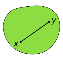
]
.pull-right[
__Not convex__

]
__Source:__ [Wikipedia](https://en.wikipedia.org/wiki/Convex_set)
---
# Convex hull
In the below example, we create a conex hull around schools; creating a polygon that includes all schools.
__Incorrect attempt__
```{r}
schools_chull1_sf <- schools_sf %>%
st_convex_hull()
nrow(schools_chull1_sf)
```
---
# Convex hull
__Correct__
```{r, out.width = "40%"}
schools_chull2_sf <- schools_sf %>%
summarise(geometry = st_combine(geometry)) %>%
st_convex_hull()
ggplot() +
geom_sf(data = schools_chull2_sf) +
geom_sf(data = schools_sf, color = "red")
```
---
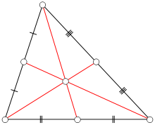
# Determine centroid
Sometimes we want to represent a polygon or polyline as a single point. For this, we can compute the centroid (ie, geographic center) of a polygon/polyline.
.center[
]
__Source:__ [Wikipedia](https://en.wikipedia.org/wiki/Centroid)
---
# Determine centroid
Determine centroid of second administrative regions
```{r, out.width = "40%"}
country_c_sf <- st_centroid(country_sf)
ggplot() +
geom_sf(data = country_c_sf)
```
---
# Remove geometry
__Incorrect approach__
```{r}
city_sf %>%
select(-geometry) %>%
head()
```
---
# Remove geometry
__Correct__
```{r}
city_sf %>%
st_drop_geometry() %>%
head()
```
---
# Grab coordinates
Create a matrix of coordinates
```{r}
schools_sf %>%
st_coordinates() %>%
head()
```
---
# Get bounding box
```{r}
schools_sf %>%
st_bbox()
```
---
# Spatial operations using multiple datasets
* `st_distance`: Calculate distances.
* `st_intersects`: Indicates whether simple features intersect.
* `st_intersection`: Cut one spatial object based on another.
* `st_difference`: Remove part of spatial object based on another.
* `st_join`: Spatial join (ie, add attributes of one dataframe to another based on location).
---
# Distances
For this example, we'll compute the distance between each school to a motorway.
```{r}
motor_sf <- roads_sf %>%
filter(highway == "motorway")
# Matrix: distance of each school to each motorway
dist_mat <- st_distance(schools_sf, motor_sf)
# Take minimun distance for each school
dist_mat %>% apply(1, min) %>% head()
```
---
# Exercise
.exercise[
**Exercise:** Calculate the distance from the centroid of each second administrtaive division to the nearest trunk road.
]
`r countdown(minutes = 2, seconds = 0, left = 0, font_size = "2em")`
--
.solution[
**Solution**:
```{r}
city_cent_sf <- city_sf %>% st_centroid()
trunk_sf <- roads_sf %>%
filter(highway == "trunk")
# Matrix: distance of each school to each motorway
dist_mat <- st_distance(city_cent_sf, trunk_sf)
# Take minimun distance for each school
dist_mat %>% apply(1, min) %>% head()
```
]
# Distances
There are multiple ways to calculate distances!
* __Great circle:__ sf, by default, uses s2 to computer distance (in meters) when data has a geographic CRS
* __Great circle:__ Other formulas beyond s2, such as Haversine, Vincenty, and Karney’s method. See the [geosphere](https://cran.r-project.org/web/packages/geosphere/geosphere.pdf) and [geodist](https://cran.r-project.org/web/packages/geodist/geodist.pdf) packages. Vincenty is more precise than Haversine, and Karney's method is more precise than Vincenty's method. Greater precision comes with heavy computation. For more information, see [here](https://rspatial.org/raster/sphere/2-distance.html).
* __Projected:__ We can use a projected CRS, where units are in meters already.
---
# Distances
.pull-left[
```{r}
# s2
st_distance(schools_sf[1,], schools_sf[2,]) %>%
as.numeric()
# Nigeria-specific CRS
schools_utm_sf <- st_transform(schools_sf, 32632)
st_distance(schools_utm_sf[1,], schools_utm_sf[2,]) %>%
as.numeric()
# World mercator
schools_merc_sf <- st_transform(schools_sf, 3395)
st_distance(schools_merc_sf[1,], schools_merc_sf[2,]) %>%
as.numeric()
```
]
.pull-right[
```{r}
# Haversine
distHaversine(
p1 = schools_sf[1,] %>% st_coordinates,
p2 = schools_sf[2,] %>% st_coordinates)
# Vincenty's method
distVincentySphere(
p1 = schools_sf[1,] %>% st_coordinates,
p2 = schools_sf[2,] %>% st_coordinates)
# Karney’s method
distGeo(p1 = schools_sf[1,] %>% st_coordinates,
p2 = schools_sf[2,] %>% st_coordinates)
```
]
---
# Intersects
For this example we'll determine which second administrative divisions intersects with a motorway.
```{r}
# Sparse matrix
st_intersects(city_sf, motor_sf) %>% print()
```
---
# Intersects
Take `max` (`FALSE` corresponds to 0 and `TRUE` corresponds to 1). So taking max will yeild if unit intersects with _any_ motorway
```{r}
# Matrix
st_intersects(city_sf, motor_sf, sparse = F) %>%
apply(1, max) %>%
head()
```
---
# Exercise
.exercise[
**Exercise:** Determine which motorways intersect with a trunk road
]
`r countdown(minutes = 2, seconds = 0, left = 0, font_size = "2em")`
--
.solution[
**Solution**:
```{r, eval = F}
trunk_sf <- roads_sf %>% filter(highway == "trunk")
motor_sf <- roads_sf %>% filter(highway == "motorway")
st_intersects(motor_sf, trunk_sf, sparse = F) %>%
apply(1, max) %>%
head()
```
]
---
# Intersection
We have roads for the full city. Here, we want to create new roads object that __only includes__ roads in one unit.
```{r, out.width = "40%"}
loc_sf <- city_sf %>%
head(1)
roads_loc_sf <- st_intersection(roads_sf, loc_sf)
ggplot() +
geom_sf(data = roads_loc_sf)
```
---
# Difference
We have roads for all of the city. Here, we want to create new roads object that __excludes__ roads in one unit.
```{r, out.width = "40%"}
roads_notloc_sf <- st_difference(roads_sf, loc_sf)
ggplot() +
geom_sf(data = loc_sf, fill = NA, color = "red") +
geom_sf(data = roads_notloc_sf)
```
---
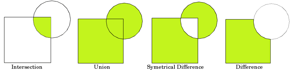
# Overlay
Intersections and differencing are __overlay__ functions
.center[
]
---
# Exercise
.exercise[
**Exercise:** Create a map of schools that are within 1km of a motorway.
]
`r countdown(minutes = 2, seconds = 0, left = 0, font_size = "2em")`
--
.solution[
**Solution**:
```{r, eval = F}
motor_1km_sf <- roads_sf %>%
filter(highway == "motorway") %>%
st_buffer(dist = 1000)
schools_nr_motor_sf <- schools_sf %>%
st_intersection(motor_1km_sf)
leaflet() %>%
addTiles() %>%
addCircles(data = schools_nr_motor_sf)
```
]
---
# Exercise
Note that there are multiple approaches we could have used for creating a map of schools that are within 1km of a trunk road.
1. Buffer trunk roads by 1km and do a spatial intersection with schools
2. Calculate the distance of each school to the nearest trunk road, then filter schools that are within 1km of a trunk road
---
# Spatial join
We have a dataset of schools. The school dataframe contains information such as the school name, but not on the administrative region it's in. To add data on the administrative region that the school is in, we'll perform a spatial join.
Check the variable names. No names of second administrative divison :(
```{r}
names(schools_sf)
```
---
# Spatial join
Use `st_join` to add attributes from `city_sf` to `schools_sf`. `st_join` is similar to other join methods (eg, `left_join`); instead of joining on a varible, we join based on location.
```{r}
schools_city_sf <- st_join(schools_sf, city_sf)
schools_city_sf %>%
names() %>%
print() %>%
tail(10)
```
---
# Spatial join
.exercise[
**Exercise:** Make a static map using of administrative areas, where each administrative area polygon displays the number of schools within the administrative area.
]
--
.solution[
**Solution**:
```{r}
## Dataframe of number of schools per NAME_2
n_school_df <- schools_city_sf %>%
st_drop_geometry() %>%
group_by(NAME_2) %>%
summarise(n_school = n()) %>%
ungroup()
## Merge info with city_sf
city_sch_sf <- city_sf %>% left_join(n_school_df, by = "NAME_2")
## Map
p <- ggplot() +
geom_sf(data = city_sch_sf,
aes(fill = n_school))
```
]
---
# Spatial join
```{r, out.width = "65%"}
ggplot() +
geom_sf(data = city_sch_sf,
aes(fill = n_school)) +
labs(fill = "N\nSchools") +
scale_fill_distiller(palette = "YlOrRd") +
theme_void()
```
---
# Spatial join
Let's outsource to [chatGPT](https://chatgpt.com/) (or [gemini](https://gemini.google.com/app) or your other favorite AI). Try entering the below prompt into chatGPT to see how it does. Does chatGPT give a correct answer? Do you need to modify chatGPT's output to make it work?
_In R, I have an sf points object of schools called schools_sf. I also have the second administrative divisions of a city as an sf polygon called city_sf and where each location is uniquely defined by the variable NAME_2. Make a static map using of administrative areas, where each administrative area polygon displays the number of schools within the administrative area. Provide R code for this._
---
# Resources
.large[
* [sf package cheatsheet](https://github.com/rstudio/cheatsheets/blob/main/sf.pdf)
* [Spatial Data Science with Applications in R](https://r-spatial.org/book/)
* [Geocomputation with R](https://r.geocompx.org/)
]
---
# Thank you!
.center[
]
---
# Load and explore polygon
The first thing we will do in this session is to recreate this data set:
```{r}
country_sf <-
st_read(here("DataWork",
"DataSets",
"Final",
"country.geojson"))
```
---
# Exploring the data
Look at first few observations
```{r, eval = T}
head(country_sf)
```
---
# Exploring the data
Number of rows
```{r, eval = T}
nrow(country_sf)
```
---
# Exploring the data
Check coordinate reference system
```{r, eval = T}
st_crs(country_sf)
```
---
# Exploring the data
Plot the data. To plot using `ggplot2`, we use the `geom_sf` geometry.
```{r, eval = T, out.width = "60%"}
ggplot() +
geom_sf(data = country_sf)
```
---
# Attributes of data
We want the area of each location, but we don't have a variable for area
```{r, eval = T}
names(country_sf)
```
---
# Attributes of data
Determine area. Note the CRS is spherical (WGS84), but `st_area` gives area in meters squared. R uses s2 geomety for this.
```{r, eval = T}
st_area(country_sf)
```
---
# Operations similar to dataframes
Create new dataset that captures locations for one administrative region
```{r, eval = T}
city_sf <- country_sf %>%
filter(NAME_1 == "Nairobi")
```
---
# Operations similar to dataframes
Plot the dataframe
```{r, eval = T, out.width = "65%"}
ggplot() +
geom_sf(data = city_sf)
```
---
# Load and explore polyline
.exercise[
**Exercise:**
* Load the roads data `roads.geojson` and name the object `roads_sf`
* Look at the first few observations
* Check the coordinate reference system
* Map the polyline
]
--
.solution[
**Solution**:
```{r, eval = F}
roads_sf <- st_read(here("DataWork", "DataSets", "Final", "roads.geojson"))
head(roads_sf)
st_crs(roads_sf)
ggplot() +
geom_sf(data = roads_sf)
```
]
---
# Load and explore polyline
```{r}
roads_sf <-
st_read(here("DataWork",
"DataSets",
"Final",
"roads.geojson"))
ggplot() +
geom_sf(data = roads_sf)
```
---
# Load and explore polyline
.exercise[
**Exercise:** Determine length of each line (hint: use `st_length`)
]
`r countdown(minutes = 1, seconds = 0, left = 0, font_size = "2em")`
--
.solution[
**Solution**:
```{r}
st_length(roads_sf)
```
]
---
# Load and explore point data
We'll load a dataset of the location of schools
```{r}
schools_df <-
read_csv(here("DataWork",
"DataSets",
"Final",
"schools.csv"))
```
---
# Explore data
```{r}
head(schools_df)
```
---
# Explore data
```{r}
names(schools_df)
```
---
# Convert to spatial object
We define the (1) coordinates (longitude and latitude) and (2) CRS. __Note:__ We must determine the CRS from the data metadata. This dataset comes from OpenStreetMaps, which uses EPSG:4326.
__Assigning the incorrect CRS is one of the most common sources of issues I see with geospatial work. If something looks weird, check the CRS!__
```{r}
schools_sf <- st_as_sf(schools_df,
coords = c("longitude", "latitude"),
crs = 4326)
```
---
# Convert to spatial object
```{r}
head(schools_sf$geometry)
```
---
# Map points object: Using sf
```{r, out.width = "50%"}
ggplot() +
geom_sf(data = schools_sf)
```
---
# Map points object: Using dataframe
```{r, out.width = "50%"}
ggplot() +
geom_point(data = schools_df,
aes(x = longitude,
y = latitude))
```
---
# Make better static map
Lets make a better static map.
```{r, out.width = "50%"}
# Adding a variable with squared km
city_sf <- city_sf %>%
mutate(area_m = city_sf %>% st_area() %>% as.numeric(),
area_km = area_m / 1000^2)
# Plotting
ggplot() +
geom_sf(data = city_sf,
aes(fill = area_km)) +
labs(fill = "Area") +
scale_fill_distiller(palette = "Blues") +
theme_void()
```
---
# Make better static map
Lets add another spatial layer
```{r, out.width = "40%"}
ggplot() +
geom_sf(data = city_sf,
aes(fill = area_km)) +
geom_sf(data = schools_sf,
aes(color = "Schools")) +
labs(fill = "Area",
color = NULL) +
scale_fill_distiller(palette = "Blues") +
scale_color_manual(values = "black") +
theme_void()
```
---
# Another static map
.exercise[
**Exercise:** Make a static map of roads, coloring each road by its type. (__Hint:__ The `highway` variable indicates the type).
]
`r countdown(minutes = 1, seconds = 0, left = 0, font_size = "2em")`
--
.solution[
**Solution**:
```{r}
ggplot() +
geom_sf(data = roads_sf,
aes(color = highway)) +
theme_void() +
labs(color = "Road Type")
```
]
---
# Another static map
```{r}
ggplot() +
geom_sf(data = roads_sf,
aes(color = highway)) +
theme_void() +
labs(color = "Road Type")
```
---
# Interactive map
We use the `leaflet` package to make interactive maps. Leaflet is a JavaScript library, but the `leaflet` R package allows making interactive maps using R. Use of leaflet somewhat mimics how we use ggplot.
* Start with `leaflet()` (instead of `ggplot()`)
* Add spatial layers, defining type of layer (similar to geometries)
```{r l1, out.height = "40%", out.width = "50%"}
leaflet() %>%
addTiles() # Basemap
```
---
# Interactive map
We use the `leaflet` package to make interactive maps. Leaflet is a JavaScript library, but the `leaflet` R package allows making interactive maps using R. Use of leaflet somewhat mimics how we use ggplot.
* Start with `leaflet()` (instead of `ggplot()`)
* Add spatial layers, defining type of layer (similar to geometries)
```{r l2, out.height = "40%", out.width = "50%"}
leaflet() %>%
addTiles() %>%
addPolygons(data = city_sf)
```
---
# Interactive map
Add a pop-up
```{r l3, out.height = "40%", out.width = "50%"}
leaflet() %>%
addTiles() %>%
addPolygons(data = city_sf,
popup = ~NAME_2)
```
---
# Interactive map
Add more than one layer
```{r l4, out.height = "40%", out.width = "50%"}
leaflet() %>%
addTiles() %>%
addPolygons(data = city_sf,
popup = ~NAME_2) %>%
addCircles(data = schools_sf,
popup = ~name,
color = "black")
```
---
# Interactive map of roads
.exercise[
**Exercise:** Create a leaflet map with roads, using the `roads_sf` dataset. (__Hint:__ Use `addPolylines()`)
]
`r countdown(minutes = 2, seconds = 0, left = 0, font_size = "2em")`
--
.solution[
**Solution**:
```{r, eval = F}
leaflet() %>%
addTiles() %>%
addPolylines(data = roads_sf)
```
]
---
# Interactive map of roads
```{r l5, out.height = "40%", out.width = "50%"}
leaflet() %>%
addTiles() %>%
addPolylines(data = roads_sf)
```
---
# Interactive maps
We can spent lots of time going over what we can done with leaflet - but that would take up too much time. [This resource](https://rstudio.github.io/leaflet/articles/colors.html) provides helpful tutorials for things like:
* Changing the basemap
* Adding colors
* Adding a legend
* And much more!
---
# Spatial operations applied on single dataset
* `st_transform`: Transform CRS
* `st_buffer`: Buffer point/line/polygon
* `st_combine`: Dissolve by attribute
* `st_convex_hull `: Create convex hull
* `st_centroid`: Create new sf object that uses the centroid
* `st_drop_geometry`: Drop geometry; convert from sf to dataframe
* `st_coordinates`: Get matrix of coordinates
* `st_bbox`: Get bounding box
---
# Transform CRS
The schools dataset is currently in a geographic CRS (WGS84), where the units are in decimal degrees. We'll tranform the CRS to a projected CRS ([EPSG:32632](https://epsg.io/32632)), and where the units will be in meters.
__Note that coordinate values are large!__ Values are large because units are in meters. Large coordinate values suggest projected CRS; latitude is between -90 and 90 and longitude is between -180 and 180.
```{r}
schools_utm_sf <- st_transform(schools_sf, 32632)
schools_utm_sf$geometry %>% head(2) %>% print()
```
---
# Buffer
We have the points of schools. Now we create a 1km buffer around schools.
```{r, out.width = "50%"}
schools_1km_sf <- schools_sf %>%
st_buffer(dist = 1000) # Units are in meters. Thanks s2!
ggplot() +
geom_sf(data = schools_1km_sf)
```
---
# Dissolve by an attribute
Below we have the second administrative regions. Using this dataset, let's create a new object at the first administrative region level.
```{r, out.width = "30%"}
country_1_sf <- country_sf %>%
group_by(NAME_1) %>%
summarise(geometry = st_combine(geometry)) %>%
ungroup()
ggplot() +
geom_sf(data = country_1_sf)
```
---
# Exercise
.exercise[
**Exercise:** Create a polyline of all trunk roads (dissolve it using `st_combine`), and buffer the polyline by 10 meters. In `roads_sf`, the `highway` variable notes road types.
]
`r countdown(minutes = 2, seconds = 0, left = 0, font_size = "2em")`
--
.solution[
**Solution**:
```{r}
roads_sf %>%
filter(highway == "trunk") %>%
summarise(geometry = st_combine(geometry)) %>%
st_buffer(dist = 10)
```
]
---
# Convex Hull
__Simple definition:__ Get the outer-most coordinates of a shape and connect-the-dots.
__Formal definition:__ A convex hull of a shape the smallest "convex set" that contains it. (A [convex set](https://en.wikipedia.org/wiki/Convex_set) is where a straight line can be drawn anywhere in the space and the space fully contains the line).
.pull-left[
__Convex__

]
.pull-right[
__Not convex__

]
__Source:__ [Wikipedia](https://en.wikipedia.org/wiki/Convex_set)
---
# Convex hull
In the below example, we create a conex hull around schools; creating a polygon that includes all schools.
__Incorrect attempt__
```{r}
schools_chull1_sf <- schools_sf %>%
st_convex_hull()
nrow(schools_chull1_sf)
```
---
# Convex hull
__Correct__
```{r, out.width = "40%"}
schools_chull2_sf <- schools_sf %>%
summarise(geometry = st_combine(geometry)) %>%
st_convex_hull()
ggplot() +
geom_sf(data = schools_chull2_sf) +
geom_sf(data = schools_sf, color = "red")
```
---
# Determine centroid
Sometimes we want to represent a polygon or polyline as a single point. For this, we can compute the centroid (ie, geographic center) of a polygon/polyline.
.center[

]
__Source:__ [Wikipedia](https://en.wikipedia.org/wiki/Centroid)
---
# Determine centroid
Determine centroid of second administrative regions
```{r, out.width = "40%"}
country_c_sf <- st_centroid(country_sf)
ggplot() +
geom_sf(data = country_c_sf)
```
---
# Remove geometry
__Incorrect approach__
```{r}
city_sf %>%
select(-geometry) %>%
head()
```
---
# Remove geometry
__Correct__
```{r}
city_sf %>%
st_drop_geometry() %>%
head()
```
---
# Grab coordinates
Create a matrix of coordinates
```{r}
schools_sf %>%
st_coordinates() %>%
head()
```
---
# Get bounding box
```{r}
schools_sf %>%
st_bbox()
```
---
# Spatial operations using multiple datasets
* `st_distance`: Calculate distances.
* `st_intersects`: Indicates whether simple features intersect.
* `st_intersection`: Cut one spatial object based on another.
* `st_difference`: Remove part of spatial object based on another.
* `st_join`: Spatial join (ie, add attributes of one dataframe to another based on location).
---
# Distances
For this example, we'll compute the distance between each school to a motorway.
```{r}
motor_sf <- roads_sf %>%
filter(highway == "motorway")
# Matrix: distance of each school to each motorway
dist_mat <- st_distance(schools_sf, motor_sf)
# Take minimun distance for each school
dist_mat %>% apply(1, min) %>% head()
```
---
# Exercise
.exercise[
**Exercise:** Calculate the distance from the centroid of each second administrtaive division to the nearest trunk road.
]
`r countdown(minutes = 2, seconds = 0, left = 0, font_size = "2em")`
--
.solution[
**Solution**:
```{r}
city_cent_sf <- city_sf %>% st_centroid()
trunk_sf <- roads_sf %>%
filter(highway == "trunk")
# Matrix: distance of each school to each motorway
dist_mat <- st_distance(city_cent_sf, trunk_sf)
# Take minimun distance for each school
dist_mat %>% apply(1, min) %>% head()
```
]
# Distances
There are multiple ways to calculate distances!
* __Great circle:__ sf, by default, uses s2 to computer distance (in meters) when data has a geographic CRS
* __Great circle:__ Other formulas beyond s2, such as Haversine, Vincenty, and Karney’s method. See the [geosphere](https://cran.r-project.org/web/packages/geosphere/geosphere.pdf) and [geodist](https://cran.r-project.org/web/packages/geodist/geodist.pdf) packages. Vincenty is more precise than Haversine, and Karney's method is more precise than Vincenty's method. Greater precision comes with heavy computation. For more information, see [here](https://rspatial.org/raster/sphere/2-distance.html).
* __Projected:__ We can use a projected CRS, where units are in meters already.
---
# Distances
.pull-left[
```{r}
# s2
st_distance(schools_sf[1,], schools_sf[2,]) %>%
as.numeric()
# Nigeria-specific CRS
schools_utm_sf <- st_transform(schools_sf, 32632)
st_distance(schools_utm_sf[1,], schools_utm_sf[2,]) %>%
as.numeric()
# World mercator
schools_merc_sf <- st_transform(schools_sf, 3395)
st_distance(schools_merc_sf[1,], schools_merc_sf[2,]) %>%
as.numeric()
```
]
.pull-right[
```{r}
# Haversine
distHaversine(
p1 = schools_sf[1,] %>% st_coordinates,
p2 = schools_sf[2,] %>% st_coordinates)
# Vincenty's method
distVincentySphere(
p1 = schools_sf[1,] %>% st_coordinates,
p2 = schools_sf[2,] %>% st_coordinates)
# Karney’s method
distGeo(p1 = schools_sf[1,] %>% st_coordinates,
p2 = schools_sf[2,] %>% st_coordinates)
```
]
---
# Intersects
For this example we'll determine which second administrative divisions intersects with a motorway.
```{r}
# Sparse matrix
st_intersects(city_sf, motor_sf) %>% print()
```
---
# Intersects
Take `max` (`FALSE` corresponds to 0 and `TRUE` corresponds to 1). So taking max will yeild if unit intersects with _any_ motorway
```{r}
# Matrix
st_intersects(city_sf, motor_sf, sparse = F) %>%
apply(1, max) %>%
head()
```
---
# Exercise
.exercise[
**Exercise:** Determine which motorways intersect with a trunk road
]
`r countdown(minutes = 2, seconds = 0, left = 0, font_size = "2em")`
--
.solution[
**Solution**:
```{r, eval = F}
trunk_sf <- roads_sf %>% filter(highway == "trunk")
motor_sf <- roads_sf %>% filter(highway == "motorway")
st_intersects(motor_sf, trunk_sf, sparse = F) %>%
apply(1, max) %>%
head()
```
]
---
# Intersection
We have roads for the full city. Here, we want to create new roads object that __only includes__ roads in one unit.
```{r, out.width = "40%"}
loc_sf <- city_sf %>%
head(1)
roads_loc_sf <- st_intersection(roads_sf, loc_sf)
ggplot() +
geom_sf(data = roads_loc_sf)
```
---
# Difference
We have roads for all of the city. Here, we want to create new roads object that __excludes__ roads in one unit.
```{r, out.width = "40%"}
roads_notloc_sf <- st_difference(roads_sf, loc_sf)
ggplot() +
geom_sf(data = loc_sf, fill = NA, color = "red") +
geom_sf(data = roads_notloc_sf)
```
---
# Overlay
Intersections and differencing are __overlay__ functions
.center[

]
---
# Exercise
.exercise[
**Exercise:** Create a map of schools that are within 1km of a motorway.
]
`r countdown(minutes = 2, seconds = 0, left = 0, font_size = "2em")`
--
.solution[
**Solution**:
```{r, eval = F}
motor_1km_sf <- roads_sf %>%
filter(highway == "motorway") %>%
st_buffer(dist = 1000)
schools_nr_motor_sf <- schools_sf %>%
st_intersection(motor_1km_sf)
leaflet() %>%
addTiles() %>%
addCircles(data = schools_nr_motor_sf)
```
]
---
# Exercise
Note that there are multiple approaches we could have used for creating a map of schools that are within 1km of a trunk road.
1. Buffer trunk roads by 1km and do a spatial intersection with schools
2. Calculate the distance of each school to the nearest trunk road, then filter schools that are within 1km of a trunk road
---
# Spatial join
We have a dataset of schools. The school dataframe contains information such as the school name, but not on the administrative region it's in. To add data on the administrative region that the school is in, we'll perform a spatial join.
Check the variable names. No names of second administrative divison :(
```{r}
names(schools_sf)
```
---
# Spatial join
Use `st_join` to add attributes from `city_sf` to `schools_sf`. `st_join` is similar to other join methods (eg, `left_join`); instead of joining on a varible, we join based on location.
```{r}
schools_city_sf <- st_join(schools_sf, city_sf)
schools_city_sf %>%
names() %>%
print() %>%
tail(10)
```
---
# Spatial join
.exercise[
**Exercise:** Make a static map using of administrative areas, where each administrative area polygon displays the number of schools within the administrative area.
]
--
.solution[
**Solution**:
```{r}
## Dataframe of number of schools per NAME_2
n_school_df <- schools_city_sf %>%
st_drop_geometry() %>%
group_by(NAME_2) %>%
summarise(n_school = n()) %>%
ungroup()
## Merge info with city_sf
city_sch_sf <- city_sf %>% left_join(n_school_df, by = "NAME_2")
## Map
p <- ggplot() +
geom_sf(data = city_sch_sf,
aes(fill = n_school))
```
]
---
# Spatial join
```{r, out.width = "65%"}
ggplot() +
geom_sf(data = city_sch_sf,
aes(fill = n_school)) +
labs(fill = "N\nSchools") +
scale_fill_distiller(palette = "YlOrRd") +
theme_void()
```
---
# Spatial join
Let's outsource to [chatGPT](https://chatgpt.com/) (or [gemini](https://gemini.google.com/app) or your other favorite AI). Try entering the below prompt into chatGPT to see how it does. Does chatGPT give a correct answer? Do you need to modify chatGPT's output to make it work?
_In R, I have an sf points object of schools called schools_sf. I also have the second administrative divisions of a city as an sf polygon called city_sf and where each location is uniquely defined by the variable NAME_2. Make a static map using of administrative areas, where each administrative area polygon displays the number of schools within the administrative area. Provide R code for this._
---
# Resources
.large[
* [sf package cheatsheet](https://github.com/rstudio/cheatsheets/blob/main/sf.pdf)
* [Spatial Data Science with Applications in R](https://r-spatial.org/book/)
* [Geocomputation with R](https://r.geocompx.org/)
]
---
# Thank you!
.center[
 ]
]