Requirements
Create an account on Google Cloud Platform (free)
You should already have done this for the lecture on Google Compute Engine. See here if not.
R packages
- New: DBI, duckdb, bigrquery, glue
- Already used: tidyverse, hrbrthemes, nycflights13
As per usual, the code chunk below will install (if necessary) and load all of these packages for you. I’m also going to set my preferred ggplot2 theme, but as you wish.
## Load/install packages
if (!require("pacman")) install.packages("pacman")
pacman::p_load(tidyverse, DBI, duckdb, bigrquery, hrbrthemes, nycflights13, glue)
## My preferred ggplot2 theme (optional)
theme_set(hrbrthemes::theme_ipsum())Databases 101
Many “big data” problems could be more accurately described as “small data problems in disguise”. Which is to say, the data that we care about is only a subset or aggregation of some larger dataset. For example, we might want to access US Census data… but only for a handful of counties along the border of two contiguous states. Or, we might want to analyse climate data collected from a large number of weather stations… but aggregated up to the national or monthly level. In such cases, the underlying bottleneck is interacting with the original data, which is too big to fit into memory. How do we store data of this magnitude and and then access it effectively? The answer is through a database.
Databases can exist either locally or remotely, as well as in-memory or on-disk. Regardless of where a database is located, the key point is that information is stored in a way that allows for very quick extraction and/or aggregation. Think back to our filing cabinet analogy from the data.table lecture:
A filing cabinet arranges items by alphabetical order: Files starting “ABC” in the top drawer, “DEF” in the second drawer, etc. To find Alice’s file, you’d only have to search the top draw. For Fred, the second draw, and so on.
This analogy, whilst slightly imperfect, captures the essence of what makes databases so efficient.1 They can very quickly identify the components that they need to focus on for a particular operation. Extracting the specific information that we want is a simple matter of submitting a query to the database. The query is where we tell the database how to manipulate or subset the data into a more manageable form, which we can then pull into our analysis environment (R, Python, etc.)
At this point, you might be tempted to think of a database as the “thing” that you interact with directly. However, it’s important to realise that the data are actually organised in one or more tables within the database. These tables are rectangular, consisting of rows and columns, where each row is identified by a unique key. In that sense, they are very much like the data frames that we’re all used to working with. Continuing with the analogy, a database then is rather like a list of data frames of R. To access information from a specific table (data frame), we first have to index it from the database (list) and then execute our query functions. The only material difference being that databases can hold much more information and are extremely efficient at executing queries over their vast contents.
Tip: A table in a database is like a data frame in an R list.
Databases and R
Virtually every database in existence makes use of SQL (Structured Query Language ). SQL is an extremely powerful tool and has become something of prerequisite for many data science jobs. (Exhibit A.) However, it is also an archaic language that is much less intuitive than the R tools that we have using thus far in the course. We’ll see several examples of this shortly, but first the good news: You already have all the programming skills you need to start working with databases. This is because the tidyverse — through dplyr — allows for direct communication with databases from your local R environment.
What does this mean?
Simply that you can interact with the vast datasets that are stored in relational databases using the same tidyverse verbs and syntax that we already know. All of this is possible thanks to the dbplyr package (link), which provides a database backend to dplyr. What’s happening even further behind the scenes is that, upon installation, dbplyr suggests the DBI package (link) as a dependency. DBI provides a common interface that allows dplyr to work with many different databases using exactly the same code. You don’t even need to leave your RStudio session or learn SQL!
Aside: Okay, you will probably want to learn SQL eventually. Luckily, dplyr and dbplyr come with several features that can really help to speed up the learning and translation process. We’ll get to these later in the lecture.
While DBI is automatically bundled with dbplyr, you’ll need to install a specific backend package for the type of database that you want to connect to. You can see a list of commonly used backends here. For today, however, we’ll focus on two:
- duckdb embeds a DuckDB database.
- bigrquery connects to Google BigQuery.
The former is a lightweight — but extremely powerful — database management system (DBMS) that can exist on our local computers. It thus provides the simplest way of demonstrating the key concepts of this section without the additional overhead required by some other common other DBMSs. (No external dependencies, no need to connect to a remote server, etc.) The latter is the one that I use most frequently in my own work and also requires minimal overhead, seeing as we already set up a Google Cloud account in the previous lecture.
Getting started: DuckDB
Our goal for this section is to create a makeshift database on our local computers — using the excellent DuckDB backend — and then connect to it from R. I’ll use this to demonstrate the ease with which we can execute queries from R, as well as underscore some principles for working with databases in general. The lessons that we learn here will carry over to more complicated cases and much larger datasets.
Connecting to a database
Start by opening an (empty) database connection via the DBI::dbConnect() function, which we’ll call con. Note that we are calling the duckdb package in the background for the DuckDB backend and telling R that this is a local connection that exists in memory.
# library(DBI) ## Already loaded
con = dbConnect(duckdb::duckdb(), path = ":memory:")The arguments to DBI::dbConnect() vary from database to database. However, the first argument is always the database backend, i.e. duckdb::duckdb() in this case since we’re using DuckDB. Again, while this differs depending on the database type that you’re connecting with, DuckDB only needs one other argument: the path to the database. Here we use the special string, “:memory:”, which causes DuckDB to make a temporary in-memory database. We’ll explore more complicated connections later on that will involve things like password prompts for remote databases.
Our makeshift database connection con is currently empty. So let’s copy across the flights dataset that comes bundled together with the nycflights13 package. There are a couple of ways to do this, but here I’ll use the dplyr::copy_to() convenience function. Note that we are specifying the table name (“flights”) that will exist within this database. You can also see that we’re passing a list of indexes to the copy_to() function. Indexes are what enable efficient database performance, since they specify how the data should be laid out for very quick search and aggregation.2 At the same time, I don’t want you to worry too much about this right now. Indexes will be set by the database host platform or maintainer in normal applications.
# library(dplyr) ## Already loaded
# library(nycflights13) ## Already loaded
copy_to(
dest = con,
df = nycflights13::flights,
name = "flights",
temporary = FALSE,
indexes = list(
c("year", "month", "day"),
"carrier",
"tailnum",
"dest"
)
)Now that we’ve copied over the data, we can reference it from R via the dplyr::tbl() function. This will allow us to treat it as a normal data frame that be manipulated with dplyr commands.
## List tables in our DuckDB database connection (optional)
# dbListTables(con)
## Reference the table from R
flights_db = tbl(con, "flights")
flights_db## # Source: table<flights> [?? x 19]
## # Database: duckdb_connection
## year month day dep_time sched_dep_time dep_delay arr_time sched_arr_time
## <int> <int> <int> <int> <int> <dbl> <int> <int>
## 1 2013 1 1 517 515 2 830 819
## 2 2013 1 1 533 529 4 850 830
## 3 2013 1 1 542 540 2 923 850
## 4 2013 1 1 544 545 -1 1004 1022
## 5 2013 1 1 554 600 -6 812 837
## 6 2013 1 1 554 558 -4 740 728
## 7 2013 1 1 555 600 -5 913 854
## 8 2013 1 1 557 600 -3 709 723
## 9 2013 1 1 557 600 -3 838 846
## 10 2013 1 1 558 600 -2 753 745
## # … with more rows, and 11 more variables: arr_delay <dbl>, carrier <chr>,
## # flight <int>, tailnum <chr>, origin <chr>, dest <chr>, air_time <dbl>,
## # distance <dbl>, hour <dbl>, minute <dbl>, time_hour <dttm>It worked! Everything looks pretty good, although you may notice something slightly strange about the output. We’ll get to that in a minute.
Generating queries
Again, one of the best things about dplyr is that it automatically translates tidyverse-style code into SQL for you. In fact, many of the key dplyr verbs are based on SQL equivalents. With that in mind, let’s try out a few queries using the typical dplyr syntax that we already know.
## Select some columns
flights_db %>% select(year:day, dep_delay, arr_delay)## # Source: lazy query [?? x 5]
## # Database: duckdb_connection
## year month day dep_delay arr_delay
## <int> <int> <int> <dbl> <dbl>
## 1 2013 1 1 2 11
## 2 2013 1 1 4 20
## 3 2013 1 1 2 33
## 4 2013 1 1 -1 -18
## 5 2013 1 1 -6 -25
## 6 2013 1 1 -4 12
## 7 2013 1 1 -5 19
## 8 2013 1 1 -3 -14
## 9 2013 1 1 -3 -8
## 10 2013 1 1 -2 8
## # … with more rows## Filter according to some condition
flights_db %>% filter(dep_delay > 240) ## # Source: lazy query [?? x 19]
## # Database: duckdb_connection
## year month day dep_time sched_dep_time dep_delay arr_time sched_arr_time
## <int> <int> <int> <int> <int> <dbl> <int> <int>
## 1 2013 1 1 848 1835 853 1001 1950
## 2 2013 1 1 1815 1325 290 2120 1542
## 3 2013 1 1 1842 1422 260 1958 1535
## 4 2013 1 1 2115 1700 255 2330 1920
## 5 2013 1 1 2205 1720 285 46 2040
## 6 2013 1 1 2343 1724 379 314 1938
## 7 2013 1 2 1332 904 268 1616 1128
## 8 2013 1 2 1412 838 334 1710 1147
## 9 2013 1 2 1607 1030 337 2003 1355
## 10 2013 1 2 2131 1512 379 2340 1741
## # … with more rows, and 11 more variables: arr_delay <dbl>, carrier <chr>,
## # flight <int>, tailnum <chr>, origin <chr>, dest <chr>, air_time <dbl>,
## # distance <dbl>, hour <dbl>, minute <dbl>, time_hour <dttm>## Get the mean delay by destination (group and then summarise)
flights_db %>%
group_by(dest) %>%
summarise(mean_dep_delay = mean(dep_delay))## Warning: Missing values are always removed in SQL.
## Use `mean(x, na.rm = TRUE)` to silence this warning
## This warning is displayed only once per session.## # Source: lazy query [?? x 2]
## # Database: duckdb_connection
## dest mean_dep_delay
## <chr> <dbl>
## 1 IAH 10.8
## 2 MIA 8.88
## 3 BQN 12.4
## 4 ATL 12.5
## 5 ORD 13.6
## 6 FLL 12.7
## 7 IAD 17.0
## 8 MCO 11.3
## 9 PBI 13.0
## 10 TPA 12.1
## # … with more rowsAgain, everything seems to be working great with the minor exception being that our output looks a little different to normal. In particular, you might be wondering what # Source: lazy query means.
Laziness as a virtue
The modus operandi of dplyr is to be as lazy as possible. What this means in practice is that your R code is translated into SQL and executed in the database, not in R. This is a good thing, since:
- It never pulls data into R unless you explicitly ask for it.
- It delays doing any work until the last possible moment: it collects together everything you want to do and then sends it to the database in one step.
For example, consider an example where we are interested in the mean departure and arrival delays for each plane (i.e. by unique tail number). I’ll also drop observations with less than 100 flights.
tailnum_delay_db =
flights_db %>%
group_by(tailnum) %>%
summarise(
mean_dep_delay = mean(dep_delay),
mean_arr_delay = mean(arr_delay),
n = n()
) %>%
filter(n > 100) %>%
arrange(desc(mean_arr_delay))Surprisingly, this sequence of operations never touches the database.3 It’s not until you actually ask for the data (say, by printing tailnum_delay_db) that dplyr generates the SQL and requests the results from the database. Even then it tries to do as little work as possible and only pulls down a few rows.
tailnum_delay_db## # Source: lazy query [?? x 4]
## # Database: duckdb_connection
## # Ordered by: desc(mean_arr_delay)
## tailnum mean_dep_delay mean_arr_delay n
## <chr> <dbl> <dbl> <dbl>
## 1 N11119 32.6 30.3 148
## 2 N16919 32.4 29.9 251
## 3 N14998 29.4 27.9 230
## 4 N15910 29.3 27.6 280
## 5 N13123 29.6 26.0 121
## 6 N11192 27.5 25.9 154
## 7 N14950 26.2 25.3 219
## 8 N21130 27.0 25.0 126
## 9 N24128 24.8 24.9 129
## 10 N22971 26.5 24.7 230
## # … with more rowsCollect the data into your local R environment
Typically, you’ll iterate a few times before you figure out what data you need from the database. Once you’ve figured it out, use collect() to pull all the data into a local data frame. I’m going to assign this collected data frame to a new object (i.e. tailnum_delay), but only because I want to keep the queried data base object (tailnum_delay_db) separate for demonstrating some SQL translation principles in the next section.
tailnum_delay =
tailnum_delay_db %>%
collect()
tailnum_delay## # A tibble: 1,201 x 4
## tailnum mean_dep_delay mean_arr_delay n
## <chr> <dbl> <dbl> <dbl>
## 1 N11119 32.6 30.3 148
## 2 N16919 32.4 29.9 251
## 3 N14998 29.4 27.9 230
## 4 N15910 29.3 27.6 280
## 5 N13123 29.6 26.0 121
## 6 N11192 27.5 25.9 154
## 7 N14950 26.2 25.3 219
## 8 N21130 27.0 25.0 126
## 9 N24128 24.8 24.9 129
## 10 N22971 26.5 24.7 230
## # … with 1,191 more rowsSuper. We have successfully pulled the queried database into our local R environment as a data frame. You can now proceed to use it in exactly the same way as you would any other data frame. For example, we could plot the data to see i) whether there is a relationship between mean departure and arrival delays (there is), and ii) whether planes manage to make up some time if they depart late (they do).
tailnum_delay %>%
ggplot(aes(x=mean_dep_delay, y=mean_arr_delay, size=n)) +
geom_point(alpha=0.3) +
geom_abline(intercept = 0, slope = 1, col="orange") +
coord_fixed()## Warning: Removed 1 rows containing missing values (geom_point).
Joins
One of the things that databases excel at are joins. At interesting touchpoint here is that dplyr’s collection of joining functions are based on their SQL equivalents (including names). You’ll hence be relieved to know that the translation carries over rather nicely for joins too. Here is a simple example, using the exact same left join that we saw back in the tidyverse lecture. Note that I’m copying over the planes data frame to the same DuckDB connection that is housing the flights table. Again, I want to emphasise that databases are like lists, in the sense that they can hold multiple datasets (i.e. tables).
## Copy over the "planes" dataset to the same "con" DuckDB connection.
copy_to(
dest = con,
df = nycflights13::planes,
name = "planes",
temporary = FALSE,
indexes = "tailnum"
)
## List tables in our "con" database connection (i.e. now "flights" and "planes")
dbListTables(con)## [1] "flights" "planes"## Reference from dplyr
planes_db = tbl(con, 'planes')
## Run the equivalent left join that we saw back in the tidyverse lecture
left_join(
flights_db,
planes_db %>% rename(year_built = year),
by = "tailnum" ## Important: Be specific about the joining column
) %>%
select(year, month, day, dep_time, arr_time, carrier, flight, tailnum,
year_built, type, model) ## # Source: lazy query [?? x 11]
## # Database: duckdb_connection
## year month day dep_time arr_time carrier flight tailnum year_built type
## <int> <int> <int> <int> <int> <chr> <int> <chr> <int> <chr>
## 1 2013 1 1 517 830 UA 1545 N14228 1999 Fixed …
## 2 2013 1 1 533 850 UA 1714 N24211 1998 Fixed …
## 3 2013 1 1 542 923 AA 1141 N619AA 1990 Fixed …
## 4 2013 1 1 544 1004 B6 725 N804JB 2012 Fixed …
## 5 2013 1 1 554 812 DL 461 N668DN 1991 Fixed …
## 6 2013 1 1 554 740 UA 1696 N39463 2012 Fixed …
## 7 2013 1 1 555 913 B6 507 N516JB 2000 Fixed …
## 8 2013 1 1 557 709 EV 5708 N829AS 1998 Fixed …
## 9 2013 1 1 557 838 B6 79 N593JB 2004 Fixed …
## 10 2013 1 1 558 849 B6 49 N793JB 2011 Fixed …
## # … with more rows, and 1 more variable: model <chr>Assuming that we’re finished querying our DuckDB database at this point, we’d normally disconnect from it by calling DBI::dbDisconnect(con). However, I want to keep the connection open a bit longer, so that I can demonstrate how to execute raw (i.e. untranslated) SQL queries on a database from within R.
Using SQL directly in R
Translate with dplyr::show_query()
Behind the scenes, dplyr is translating your R code into SQL. You can use the show_query() function to display the SQL code that was used to generate a queried table.
tailnum_delay_db %>% show_query()## <SQL>
## SELECT *
## FROM (SELECT "tailnum", AVG("dep_delay") AS "mean_dep_delay", AVG("arr_delay") AS "mean_arr_delay", COUNT(*) AS "n"
## FROM "flights"
## GROUP BY "tailnum") "q01"
## WHERE ("n" > 100.0)
## ORDER BY "mean_arr_delay" DESCNote that the SQL call is much less appealing/intuitive our piped dplyr code. In part, this is an artefact of the translation steps involved. The dplyr translation engine includes various safeguards that are designed to ensure that the resulting SQL code works. But this comes at the expense of code concision (e.g. those repeated SELECT commands at the top of the SQL string are redundant). However, it also reflects the simple fact that SQL is not an elegant language to work with. In particular, SQL imposes a lexical order of operations that doesn’t necessarily preserve the logical order of operations.4 This lexical ordering is also known as “order of execution” and is strict in the sense that every SQL query must follow the same hierarchy of commands. Here is how Julia Evans lays it out in her wonderful zine, Become A Select Star (which you should totally buy).
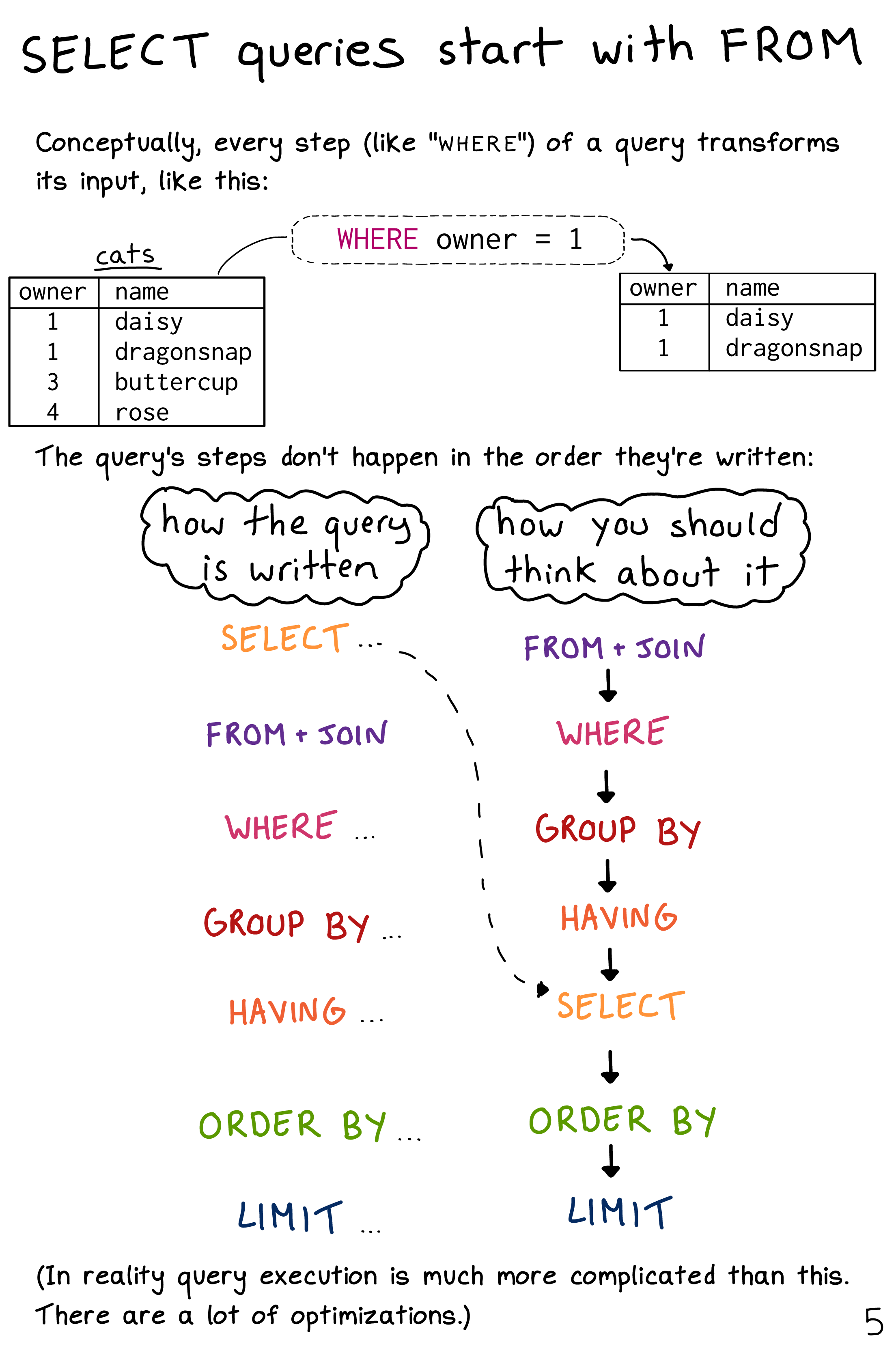.)](data:image/png;base64,iVBORw0KGgoAAAANSUhEUgAACKAAAA0WEAYAAADM2MuDAAAJJmlDQ1BpY2MAAEiJlZVnUJNZF8fv8zzphUASQodQQ5EqJYCUEFoo0quoQOidUEVsiLgCK4qINEWQRQEXXJUia0UUC4uCAhZ0gywCyrpxFVFBWXDfGZ33HT+8/5l7z2/+c+bec8/5cAEgiINlwct7YlK6wNvJjhkYFMwE3yiMn5bC8fR0A9/VuxEArcR7ut/P+a4IEZFp/OW4uLxy+SmCdACg7GXWzEpPWeGjy0wPj//CZ1dYsFzgMt9Y4eh/eexLzr8s+pLj681dfhUKABwp+hsO/4b/c++KVDiC9NioyGymT3JUelaYIJKZttIJHpfL9BQkR8UmRH5T8P+V/B2lR2anr0RucsomQWx0TDrzfw41MjA0BF9n8cbrS48hRv9/z2dFX73kegDYcwAg+7564ZUAdO4CQPrRV09tua+UfAA67vAzBJn/eqiVDQ0IgALoQAYoAlWgCXSBETADlsAWOAAX4AF8QRDYAPggBiQCAcgCuWAHKABFYB84CKpALWgATaAVnAad4Dy4Aq6D2+AuGAaPgRBMgpdABN6BBQiCsBAZokEykBKkDulARhAbsoYcIDfIGwqCQqFoKAnKgHKhnVARVApVQXVQE/QLdA66At2EBqGH0Dg0A/0NfYQRmATTYQVYA9aH2TAHdoV94fVwNJwK58D58F64Aq6HT8Id8BX4NjwMC+GX8BwCECLCQJQRXYSNcBEPJBiJQgTIVqQQKUfqkVakG+lD7iFCZBb5gMKgaCgmShdliXJG+aH4qFTUVlQxqgp1AtWB6kXdQ42jRKjPaDJaHq2DtkDz0IHoaHQWugBdjm5Et6OvoYfRk+h3GAyGgWFhzDDOmCBMHGYzphhzGNOGuYwZxExg5rBYrAxWB2uF9cCGYdOxBdhK7EnsJewQdhL7HkfEKeGMcI64YFwSLg9XjmvGXcQN4aZwC3hxvDreAu+Bj8BvwpfgG/Dd+Dv4SfwCQYLAIlgRfAlxhB2ECkIr4RphjPCGSCSqEM2JXsRY4nZiBfEU8QZxnPiBRCVpk7ikEFIGaS/pOOky6SHpDZlM1iDbkoPJ6eS95CbyVfJT8nsxmpieGE8sQmybWLVYh9iQ2CsKnqJO4VA2UHIo5ZQzlDuUWXG8uIY4VzxMfKt4tfg58VHxOQmahKGEh0SiRLFEs8RNiWkqlqpBdaBGUPOpx6hXqRM0hKZK49L4tJ20Bto12iQdQ2fRefQ4ehH9Z/oAXSRJlTSW9JfMlqyWvCApZCAMDQaPkcAoYZxmjDA+SilIcaQipfZItUoNSc1Ly0nbSkdKF0q3SQ9Lf5RhyjjIxMvsl+mUeSKLktWW9ZLNkj0ie012Vo4uZynHlyuUOy33SB6W15b3lt8sf0y+X35OQVHBSSFFoVLhqsKsIkPRVjFOsUzxouKMEk3JWilWqUzpktILpiSTw0xgVjB7mSJleWVn5QzlOuUB5QUVloqfSp5Km8oTVYIqWzVKtUy1R1WkpqTmrpar1qL2SB2vzlaPUT+k3qc+r8HSCNDYrdGpMc2SZvFYOawW1pgmWdNGM1WzXvO+FkaLrRWvdVjrrjasbaIdo12tfUcH1jHVidU5rDO4Cr3KfFXSqvpVo7okXY5upm6L7rgeQ89NL0+vU++Vvpp+sP5+/T79zwYmBgkGDQaPDamGLoZ5ht2GfxtpG/GNqo3uryavdly9bXXX6tfGOsaRxkeMH5jQTNxNdpv0mHwyNTMVmLaazpipmYWa1ZiNsulsT3Yx+4Y52tzOfJv5efMPFqYW6RanLf6y1LWMt2y2nF7DWhO5pmHNhJWKVZhVnZXQmmkdan3UWmijbBNmU2/zzFbVNsK20XaKo8WJ45zkvLIzsBPYtdvNcy24W7iX7RF7J/tC+wEHqoOfQ5XDU0cVx2jHFkeRk4nTZqfLzmhnV+f9zqM8BR6f18QTuZi5bHHpdSW5+rhWuT5z03YTuHW7w+4u7gfcx9aqr01a2+kBPHgeBzyeeLI8Uz1/9cJ4eXpVez33NvTO9e7zofls9Gn2eedr51vi+9hP0y/Dr8ef4h/i3+Q/H2AfUBogDNQP3BJ4O0g2KDaoKxgb7B/cGDy3zmHdwXWTISYhBSEj61nrs9ff3CC7IWHDhY2UjWEbz4SiQwNCm0MXwzzC6sPmwnnhNeEiPpd/iP8ywjaiLGIm0iqyNHIqyiqqNGo62ir6QPRMjE1MecxsLDe2KvZ1nHNcbdx8vEf88filhICEtkRcYmjiuSRqUnxSb7JicnbyYIpOSkGKMNUi9WCqSOAqaEyD0tandaXTlz/F/gzNjF0Z45nWmdWZ77P8s85kS2QnZfdv0t60Z9NUjmPOT5tRm/mbe3KVc3fkjm/hbKnbCm0N39qzTXVb/rbJ7U7bT+wg7Ijf8VueQV5p3tudATu78xXyt+dP7HLa1VIgViAoGN1tubv2B9QPsT8M7Fm9p3LP58KIwltFBkXlRYvF/OJbPxr+WPHj0t6ovQMlpiVH9mH2Je0b2W+z/0SpRGlO6cQB9wMdZcyywrK3BzcevFluXF57iHAo45Cwwq2iq1Ktcl/lYlVM1XC1XXVbjXzNnpr5wxGHh47YHmmtVagtqv14NPbogzqnuo56jfryY5hjmceeN/g39P3E/qmpUbaxqPHT8aTjwhPeJ3qbzJqamuWbS1rgloyWmZMhJ+/+bP9zV6tua10bo63oFDiVcerFL6G/jJx2Pd1zhn2m9az62Zp2WnthB9SxqUPUGdMp7ArqGjzncq6n27K7/Ve9X4+fVz5ffUHyQslFwsX8i0uXci7NXU65PHsl+spEz8aex1cDr97v9eoduOZ67cZ1x+tX+zh9l25Y3Th/0+LmuVvsW523TW939Jv0t/9m8lv7gOlAxx2zO113ze92D64ZvDhkM3Tlnv296/d5928Prx0eHPEbeTAaMip8EPFg+mHCw9ePMh8tPN4+hh4rfCL+pPyp/NP637V+bxOaCi+M24/3P/N59niCP/Hyj7Q/Fifzn5Ofl08pTTVNG02fn3Gcufti3YvJlykvF2YL/pT4s+aV5quzf9n+1S8KFE2+Frxe+rv4jcyb42+N3/bMec49fZf4bmG+8L3M+xMf2B/6PgZ8nFrIWsQuVnzS+tT92fXz2FLi0tI/QiyQvpNzTVQAAAAgY0hSTQAAeiYAAICEAAD6AAAAgOgAAHUwAADqYAAAOpgAABdwnLpRPAAAAAZiS0dE////////CVj33AAAAAlwSFlzAAABLAAAASwAc4jpUgAAAAd0SU1FB+QBHw4GBVi1404AAIAASURBVHja7N2tb11dejfgk9GggkoxalXyyJ6C0sassDEusllHBa9sqf9AQkclNiq2VdKysemwBBU7pQWVoyHVMEdt8TQvcH/yPOvJic/HWnvtj+sie5x54uyzz97r877v/err/1kBAAAAAAAAAAAAAAAAAAAAAAzsZ71PAAAAAAAAAAAAAAAAAAAAAABYLgVQAAAAAAAAAAAAAAAAAAAAAIBuFEABAAAAAAAAAAAAAAAAAAAAALpRAAUAAAAAAAAAAAAAAAAAAAAA6EYBFAAAAAAAAAAAAAAAAAAAAACgGwVQAAAAAAAAAAAAAAAAAAAAAIBuFEABAAAAAAAAAAAAAAAAAAAAALpRAAUAAAAAAAAAAAAAAAAAAAAA6EYBFAAAAAAAAAAAAAAAAAAAAACgGwVQAAAAAAAAAAAAAAAAAAAAAIBuFEABAAAAAAAAAAAAAAAAAAAAALpRAAUAAAAAAAAAAAAAAAAAAAAA6EYBFAAAAAAAAAAAAAAAAAAAAACgGwVQAAAAAAAAAAAAAAAAAAAAAIBuFEABAAAAAAAAAAAAAAAAAAAAALpRAAUAAAAAAAAAAAAAAAAAAAAA6EYBFAAAAAAAAAAAAAAAAAAAAACgGwVQAAAAAAAAAAAAAAAAAAAAAIBuFEABAAAAAAAAAAAAAAAAAAAAALpRAAUAAAAAAAAAAAAAAAAAAAAA6EYBFAAAAAAAAAAAAAAAAAAAAACgGwVQAAAAAAAAAAAAAAAAAAAAAIBuFEABAAAAAAAAAAAAAAAAAAAAALpRAAUAAAAAAAAAAAAAAAAAAAAA6EYBFAAAAAAAAAAAAAAAAAAAAACgGwVQAAAAAAAAAAAAAAAAAAAAAIBuFEABAAAAAAAAAAAAAAAAAAAAALpRAAUAAAAAAAAAAAAAAAAAAAAA6EYBFAAAAAAAAAAAAAAAAAAAAACgGwVQAAAAAAAAAAAAAAAAAAAAAIBuFEABAAAAAAAAAAAAAAAAAAAAALpRAAUAAAAAAAAAAAAAAAAAAAAA6EYBFAAAAAAAAAAAAAAAAAAAAACgGwVQAAAAAAAAAAAAAAAAAAAAAIBuFEABAAAAAAAAAAAAAAAAAAAAALpRAAUAAAAAAAAAAAAAAAAAAAAA6EYBFAAAAAAAAAAAAAAAAAAAAACgGwVQAAAAAAAAAAAAAAAAAAAAAIBuFEABAAAAAAAAAAAAAAAAAAAAALpRAAUAAAAAAAAAAAAAAAAAAAAA6EYBFAAAAAAAAAAAAAAAAAAAAACgGwVQAAAAAAAAAAAAAAAAAAAAAIBuFEABAAAAAAAAAAAAAAAAAAAAALpRAAUAAAAAAAAAAAAAAAAAAAAA6EYBFAAAAAAAAAAAAAAAAAAAAACgGwVQAAAAAAAAAAAAAAAAAAAAAIBuFEABAAAAAAAAAAAAAAAAAAAAALpRAAUAAAAAAAAAAAAAAAAAAAAA6EYBFAAAAAAAAAAAAAAAAAAAAACgGwVQAAAAAAAAAAAAAAAAAAAAAIBuFEABAAAAAAAAAAAAAAAAAAAAALpRAAUAAAAAAAAAAAAAAAAAAAAA6EYBFAAAAAAAAAAAAAAAAAAAAACgGwVQAAAAAAAAAAAAAAAAAAAAAIBuFEABAAAAAAAAAAAAAAAAAAAAALpRAAUAAAAAAAAAAAAAAAAAAAAA6EYBFAAAAAAAAAAAAAAAAAAAAACgGwVQAAAAAAAAAAAAAAAAAAAAAIBuft77BAAAAAAAAAAAAAAAAGDKPn369OnTp9Xqy5cvX758Wa1ev379+vXr1erNmzdv3rzpfXYAAAAA4/ez3icAAAAAAAAAAAAAAADAbj5//vz58+fV6v379+/fv1+t7u7u7u7uep/V/OU6Hx0dHR0drVbHx8fHx8er1cnJycnJyfPP+f8/fvz48ePH3mcNAAAAMF6vvv6f3icCAAAAAAAAAAAAAADA93358uXLly/PBU9ubm5ubm5++t8dHh4eHh6uVm/fvn379u1qdXl5eXl5uVq9fv369evXvT/FdOV6X1xcXFxcbP/3b29vb29vV6vT09PT09PenwYAAABgPBRAAQAAAAAAAAAAAAAAmIiTk5OTk5PV6uPHjx8/ftz876XwyfX19fX1tQIc2/r8+fPnz59Xq6Ojo6Ojo91/T76Hh4eHh4cHBWkAAAAA4ue9TwAAAAAAAAAAAAAAAIDvS8GTbQufxJcvX758+bJaXVxcXFxcrFZv3rx58+bNanV4eHh4eNj7043f3d3d3d3d/r8n38PNzc3Nzc1q9e7du3fv3vX+dAAwLp8+ffr06dNzv7mpt2/fvn37tvfZAwCwKwVQAAAAAAAAAAAAAAAARi4FM/aVROKrq6urq6vV6vr6+vr6uvenG78kYteybUI3AMxJCoulf02Bt1r97evXr1+/fr1anZ6enp6ePhccU/gNAGDcFEABAAAAAAAAAIARS4JbAsCTIFUGcOcIQF+fP3/+/Pnz8zHSbr958+bNmze9zxIAmKLaBTOSeHx5eXl5efk8XuHbFCwBgO1lfSTr3Bl/lOsmtaXfzr+b4/n5+fn5uYIoAABj9bPeJwAAAAAAAAAAADxLYPbx8fHx8fFqdXFxcXFx8RwYnkIo+fns7Ozs7Oz5v5eQBTCstLvv379///79anV0dHR0dLRanZycnJycPB/TTufn1ok+AAAvyTgm80sAgH1lfJF17ayTXF1dXV1d9V8PSSGUnFfWc6yrAwCMgwIoAAAAAAAAAAAwIkmM//Tp06dPnzb/e/nvUxAFgGGk3U4iz0tSyCoFUXon/gAA0/H27du3b9/W/73bzj+p4/Xr169fv+59FgBQR9ZFUlgkhUbGLueddZqs2wCwLCmElX4gR+v3MDwFUAAAAAAAAAAAYAQSSLdv4lkZmAdAG3lD8K7tdvlGZACAl5yfn5+fn69Wh4eHh4eH9X7v3d3d3d1d7083frUT3968efPmzZvenwoAdpN1jRSGzTpJ/nxq0s+XnweAeUq7n/Y+BbzSD+SYP89x6v0dTIECKAAAAAAAAAAAMAK1C5YogALQVq12Nr9HwDQA8JLXr1+/fv36uRBKLeWbrvk2b/4GqCPtaVnIuVaBaNoqC5/MdfxwdXV1dXW1Wp2dnZ2dnVm3AZiLFDA5Pj4+Pj5+bu9fauczfsl/n4Io+Rmo5+e9TwAAAAAAAAAAAKhPogBAW7Xb2fy+t2/fvn37tvenAwDGrNV4IQnMxiMAy5YE33XHKOfF6/672g4PDw8PD5+PKRCWn9+8efPmzZvV6vT09PT0tPfVnI+y8MlS1p/v7u7u7u6e7+sPHz58+PDh+b4DYBouLi4uLi5Wq5ubm5ubm/1/X/rFFFTJz5eXl5eXl70/LUybAigAAAAAAAAAADBDc33zJgAAwNIlsTuJ3rUSzc0jAeYpCbkpWJH2Pn+efmQq/cCmhVbSXypYsZ+lFj4p5XPnOlxfX19fXz/fZ8D0rOsXI4UhFYicthQ8qVX4ZJ2rq6urq6vV6vz8/Pz8/Hm+DmxPARQAAAAAAAAAABiBVoHSCeAUiA0AADAvp6enp6enz4lW+8r8MYl/EsUBpqEsYFImdNcqlDU1ZcEKhVB28/79+/fv3y+38Ekp1+Hs7Ozs7Gy1ur+/v7+/d1/BlKRde2kelf8/BVD+6q/+6q/+6q9Wq9/85je/+c1vftouZh8u//27d+/evXunfegl459830O5u7u7u7t7/v6B7f2s9wkAAAAAAAAAAADt3iA3lTe3AgAAsJ1WhS7NIwE2k/YyhRBevXr16tWr52MKb+SYBNxdC5KkQFUSso+Pj4+Pj1ero6Ojo6Oj1eri4uLi4mK1urm5ubm5WW7hk1IS1GsVDJub3Fe5b3K//vmf//mf//mfP/95bykgkHX0Vuvpm8rzlesFjN+mhU9K6e9/9atf/epXv1pfEKrsb9I+pJ1lWBkXDX39UwAF2N2rr/+n94kAAAAAAAAAAADPCQu1EhTOz8/Pz89Xq+vr6+vr696fDmA+ktBWS95E3TuBBwCYntrjkryp+vLy8vLysvenGw/jPyBSECKJtbvKel3W717695K4LZF6Nymg8fj4+Pj42Pts+st9lAT9dQn9Q0lht9PT09PT0+efN+0nc/55XoYu3GL8NA+5j15qZ3N/pl1hGg4ODg4ODobvR3O/ZPzvvmkrBWgybupF9QbY3c96nwAAAAAAAAAAAPCsduJT78B1AAAA2qo9j8wbzgH4sVqFTyK/Z936Xdrj/HcKn+zH9fvxdUgh7l7rx2VBgPv7+/v7++dCItuOb/L7Ulgov/fw8PDw8LD950nCvfX4ccv3k8IIKQCUQnfHx8fHx8fPf77umEIaeY4UqBq3u7u7u7u7ft9Ped/RRl4skfa4N/Nq2J0CKAAAAAAAAAAAMCK1A7IFXAMAAMxbEn5ryTxSAifAk7IQSW3rfm8KrkBNua969fPn5+fn5+fPBUpqF3KL/N4UVjk9PT09PW3/+c7Ozs7Oztr/O2wm93sKlaTASQok7FugoCy4kH9nLAUYeDKWfbLahdT4sbEVIkr7AGxPARQAAAAAAAAAABiR2olr4U1jAAAA89Qqcdg8EuBJ60T2JGaXBU/u7u7u7u56f/r5SOGNpevVv19eXl5eXq5W19fX19fXq9Xr169fv37d/t/Nv3N7e3t7e9v+PigLYjCstKcpdJJCE0MVIkjhhRRiODk5OTk52b8AR/5+nt/0FwosbGYsBVAi359CZ3VkvDS2cdPY7juYEgVQAAAAAAAAAABgRFolrgm0AwAAmCfzSIC2hioYoWBCGymA8e7du3fv3vU+m+XJdR/L9U8BltaFUPI8pyAGbaWQRAqfjGUcm/5j20Io+e+Ojo6Ojo6eP1d+Twq75P/PnyuIMi35Hsdyv05N7vdcx7HxvcLuFEABAACACcvCXRbIc7RgBgAAAADT9+bNmzdv3tT7fQJfAQAA5q12IRTxJwDDyvpdEvnZTwqffPjw4cOHD6vV4eHh4eFh77Pqb6jrcHp6enp6ulpdXl5eXl72/tQ/1boQSgqfvH///v37970/7Xyl8MFYCyBE7ocUMlnXzqcf2LagSeLH8/vtB01Lvm8Fk7ZzdnZ2dnY23uuW+fRYzw/G7Oe9TwAAAAB4XnjOAlcZQJKfsyC96cJ0AltSOb/VG38AAAAAgPpSAKVWwpnENQAAgHnLPDJxKPuq9XvmIon0EthgeYZ+/q+urq6urp4LSNzd3d3d3Q3/udOv5POXBZtTSKMsqLHuz3dVxk2Wx6x75t/Leeb65fwZ1lgLn5RSCCX3Ue119BS6SByvQjx1pODJVAtG5fzTXuWY9n/X/iZ/L78/BaAYt3xvKYRyf39/f3/f+6zGK4WlprLvmfOUxwGbUwAFAAAAKli3oZYFyfx5fh4qQCT/To5ZyLaABgAAAADjVzsQeiqBgAAAAOwm8SBJnKwlcSdLjzepXWAGmI4U0hgq0T7xhr/61a9+9atf/fQFa7tKIZC052XBkPLnsahdUGXpNn0B367Oz8/Pz8+n933d3t7e3t6uVsfHx8fHx/ULHmV8loIrbCffRwofTLXwSSkFLxLfXavgVfqN7AuNrV0f2lTao3xfuc+nUkhqKHnua893WzOfhu0pgAIAwI9kwlwm8JemujAJ8JIyQKH8uWwnW28E1XZ2dnZ2drZaPT4+Pj4+9j4bAAAAAOB7WgWkCngFAACYp1bzPAlbbbiuMB1JQE5ieu3CCOv853/+53/+538+J8Yn/u+luMUUOnn37t27d++eC7iI+2YIyTOYmjwfeW5SgKCWtB9pT/KcspmLi4uLi4t6BULGIv1J2vfa/UsKRiy98E7t5+2P//iP//iP/3i1+u///u///u//rn++KfCR+V368aXKvmbagVbKeVmtwpdeUAHbUwAFAGDmMuEqE/UzgcoCybYTqkyos8Cnsug8vDRBt9HKFJTtWtn+5Vj+d0NtSPaWz5kF7aluNAEAAADAErRKXFvKeigAAMDSJLEv88laiVZTe0EQQG1pX1OIJAm4rRNak+ifeO2Hh4eHh4fnPy//fYnS9JQCIlMvvJ3nLXG2tcZBWZdPHob8i83MtfBJqdV4O/dx7uulFsKq/blT+CS/t9X3l/s/7erSvr9c15OTk5OTk3b/TsZ5t7e3t7e3z+20AijQjwIoAAATUSbulxOpTIiGTuTPxC7/3tIrw45N7ofcL+X9se+EvFyozs8plKJgCvtYV6jppZ/ZjMAUAAAAABi/BNzlWGv/xxumAQAA5i3zvVrxNLUSvwCmLvGy9/f39/f3z+1jjuULyvZVvggucbopcKLQCbvIfVy7f5/benPyImon3qeQhwIo35d2tFZ7uq3yfp76CzdzHZd637UqHPKP//iP//iP/7ha/c3f/M3f/M3f1P/9ud/Ozs7Ozs6exx9zV37u1s9d2vuyoGjtz5N2ZOqFwmAICqAAAHRSLkiXP9cqUDEUlWH7ykJo7pf83HqiXxbmiRTGyQJANljOz8/Pz89N2JembMfWFXBadz/RRp5PAAAAAGD8WgWkAwAAvKRMPEycR+IOkhiYuDFxQeNQO34vcWhlAj7A0pUvDKxdACUSF5z+FsZobnGpea4zvq1VWK58Ie7cCsfsK9fn/fv379+/H+7fTfua47r7Oed3cXFxcXExnX2bpRfeaTVP/aM/+qM/+qM/ei6gkfuitrQ/eS7m/j2m8FTrF+TmeS8LyrW6XxRAgc0pgAIwcesShVtVnAPWy8JF+VyWx9YTsN6WXhm2tWyMpMBIFqLGWjCi3MjJMQu1uU/0V9NQvqGgrGRdtnNTrXC9FN78AAAAAADTUTuxbO77VQAAwP6ScLQuoS9xIYlfyjGJX3lREn20TthSAAXg28o8jtoFE2DM5lrII+Pa2oUNMn6e63XbVQo8tI5DTzud+cum4+eMgz98+PDhw4fn+6J24avall54p1WBplzP5MWk3291PySPKPfr3PIB8jy13sfM9VuX95bnPMda4zDjOdicAigAI1UmFpeFFfLnLw18MtC6vb29vb2VYA7bKJ+zl36GlrLAmQW9qd936dcSKJEFQP1UW+X4oizQpJDJMmQjRiAKAAAAAExH7cBMBVAAAIB1Ep+065vMk7CUOCDxQH3kumc+WSv+J/PJuSXabUq8DbCpJJbXWofbtV8G9pe429qFOTzXP5brkbyJVjKOTeGTffdf8nvS3o99/2XphXfyuWs9f2V7MNT9kHl35idTn3cPVUgoz3vybF+S61orf2vs7QOMiQIojMq6gg9lImaUCZnlQm2O6cgzQFnqAI1xWFdAoTzWmhDn3zk+Pj4+Pn4eoC114wFWq+f+ZV0BAAtJjEH6gbOzs7Ozs/nel+XnfHh4eHh46H1W01GOl8t2LX8+1/uH7bxUqRgAAAAAGK/EOeTNbvtS+BqgjtpvgASAnjJPqDXvSOJSEsDoI/EiteKHlp6wpUApsKnaBZPKeHcFmWB4KYRSa7xc5pVNvYDBvlIAoZV8f63mJ8nXS/7eWPdhUgBlqfO0Vv1zqfX9kN+X5yYvJK49X2ltqMInkeu06X1Q+36R1wObUwCFLjIwz4CpTETf9/eukwlGOvIMXCUA7ifXPde3TMRNR5+CG+/evXv37t30BlTr5POWC0plIZOxLFCn4qgCKMzRusJCtfoZNpP+ld1kfJSJ/FgXvmorCxAtrWBdOW5YVwiwdqE05q0sAJlxOAAAAAAwPa321wVWA+xHARQA5qR2fJ3EnnFQAAWgj1ZxsAqgMGZzyRNbJ3lYtQqgxNLX6XM9W62vDfUCybTLiddO/t7YJA8heStLyy+s3U6tm2flfkihmbwwuLa0H7nfplLYZujCJ7ku27aztV9QEUvNm4JtKIBCUxl4piPKwKj3hm9ZoTwdxlQrnfWS63hycnJycrI+ETffd3m9dx041FYWLimPc0s8zudY6kSFecj9WxbU6t2/LF0Waiyobyf9SRYchprAj9XcJvLleHisBdIYp7SnOZbj5vyc+ctcnhsAAAAA4Kda7atPdd8bYK60ywDMiX5tHGrPJ8u4avGCAN+W9jHxfbX6xbnF2TIvvfPDhvp8tZ/rpebBlPmdteV7GjpfNHk1Zd7T2KQ/WVpeYauCFuvmR7m+uS9a3e/JVykL8YxFmYc81HOR67Dri75b9Wv5/MZzsJ4CKFSVgU8GaFNJ4J1qpbNeNi18sk6udyq13d/f39/f734e5YCnrJxXLrSXx6XKdZvKRGXd91YmBjNPZbsx1gWApcpEsHVF3LnpNYFnGBmPpFKvgI5ly8JUFs7Ljc0sjBnXAAAAAAAvqR1YLcAOYFymFs8DwLzUjlcwzxiH1glbS4tzqf15lx7PDkuQdrjMc9mVeFRqWFr/XVvWbWrlTS41jyCFIFq1a8kPHarwybp///j4+Pj4ePh//yW1+qWpadX+vVQgMvlWue6tnvvkR2f80Xte3itvqlaeW5nvUev8zQPhZQqgsJc0tElIn/rAJxOPdGy9BrhjlwnGvh12/v7f/d3f/d3f/d1q9Sd/8id/8id/8nxflROYqd9fYzP2BYt8/xl4v7QwkM9ze3t7e3s7/8qxS7FvwSXqKBPyy4lw7wnx1KT/c19/29Tvp4xjFD6Zl3XtYJQV3ad+HwMAAAAA4yVhAgAAaCVxEYl72HfeoaDXOJQv6qldUHNp37MCKMC2aq/naTeo4fe///3vf//73mcxXfKV9pPxaK0CMqWMT3uPU3OfvHv37t27d8/5mGOR/iTj+qXc163mR+nnX8ojSN5jCuO02qdLPsuHDx8+fPgw/Pfbq/BJPmftF3zXLoCy1MJXsA0FUNjKtgUJpsobjp7c3d3d3d09D8AysP23f/u3f/u3f6v37/zzP//zP//zP/f+tMvTeyL3kgy0N13oy/2ZCUAG6Et/jqfu//2///f//t//E3hZWyZeZUJ/efT81JVxUwrHjc26+yLyHKa9rV2YbC73Xb5f7dY4lYVKNv0ZAAAAAGAsar/IRcIEAABQSkLW0dHR0dHR9nEwedPy2ONUl6Z2Ar6ELYA+tL/U8D//8z//8z//0/sspivj3Fp5AUt7YXgKgdSOt8/+Se3CB/tKAZTkaY5tXybntbS4+V4vHEjezPX19fX19XP+ZG05n7RTybOsvc+47t/tVfik1eesXQjTeA5epgAKG0lH7k3285bvddvCE0xLJk6tB6y7SoGAfe+/FGq6v7+/v7/v/anYVCbymWBph76vTNAvK5GmkIRE/r7GVvgkC665P/Lzrv1CPl9ZOG1T+XcTODFV+dzarWEcHBwcHBysVn/913/913/91+sLOZUFTQAAAGAMEshQvlGpLEC7q3IdcN364NQL0QIsVe0AO/EfAABAKetJDw8PDw8Pz3FPiQ9a998nPjVHxkUBlDpqz8sj11OcJ8xP9mOS8L8v63nU8F//9V//9V//Vf/35v6ce9xuPl+OnsvtrJtX7CuFGFuN13ZV5kvkxd+7/p4caxVSWWr+Q+/5UfJ4Mn+uNU5Yd14pSNIqz7L8d4ZqF1sXPin/ndpy/4nfgZ9SAIXvSgGBVh0o46LwybxlIDS2Spal2hMHGwLTkIl3JvJLXQB6KXE/P0von4behU9yf2Qhr9WCXvn7046XBa3yXOffLxdspn4/Z9zMMP7yL//yL//yL6dfOAcAAMYg6zKZv+XnrCdah4D9ZZ0k+22t3+i06zp7WVC5XKcsfwZgHpa6LwcAALysTNTL/CFxmV7MNS21v6fcD0MnOve+D1sl1Jqfw3y1ah/lSbCP3//+97///e/r/97cl0tJ5K5dQGHusm9ee7+8LMg4VmWhhuRxvjQOzPgz87IUkKmV71u+wGVsBWRaqd0/71ogMnme+fut2pP8/uQ3XV9fX19f1/u9cy18Eq36taX1m7ANBVD4kXQw6XCWVpl5qQvxGfiacM1LBj5JME9i+lhlolS7kmfu66U911OTiffcNnDKxAAJA8vQu/BJ2vss4A29AJX+ZykT8PQzSxs3x7r2LXIf/Md//Md//Md/rFZ///d///d///f7/7tz6y8AAGBIWX9LIcd1gSVZrykLbI69wDKMwabP2dhsuk9UFly3vgkwrNpvjF3q+jYAALC9rBcvJS5oblrFke2bsFW+YCu/Lz9nfbX885L9DGCsWu2jiKNkH16AQg+188Viai9kzbj58fHx8fHx+bqU+zXpP5IXGK3iDzIuH3v+YS2t+uddC5SlwE1eLN7qe06+U+xaCGUphU/W/fu19lenEk8EPSiAwmq1em4oUzluqQEu6bCnMuCtZanf91SVb14tE46nGmjcaiLr/p6GcgI1Vgqa8D29Cp/kvss4RoDBsGoFmPdWvtF93c9l+9fLUitNAwDAPnadt2aDOvOfjL+XEvAAm8hzkn22uRecz+dLIEsCS6yLAgAAAMB4tVq/+/Wvf/3rX//6+edyfbSM4221flruZ+TnWm82L9VOfPPmb2BbEmbZRwoq5IUO0FLGf7XHgWUBvKnK81gWOnnpv69NAZQ60j9v+/tzP6cQSuvCIrsWQllq4ZPyPBRAgfYUQFm4NJCpDDaWCqDpCLKAt2miZT5PBlwvFVRIR5cOutUAcOwUiOhrXSGFpRVUaNX+GAiOW+/2p0zsn1thIYbRq/BJKhVPrWLx3PRux0pjLWTSamM+z583tgAAwHpZH6s1b83vKdfvYYmyH5XCJ2PZZxtKPm8CIxNoAkBbrfYDehWcXhfwXL7Zu4wjsS8CAACwm8yraiWg/tM//dM//dM/PR/HInFFmU/WTuSsPS9d2voyLFHt9leeBPvIOvAPP/zwww8/rFa//e1vf/vb3+7/e3N/K+i1nbnHXbR6YXbGd0vdL0gebK3rO/cXvZRy3+RYazye/a1d85Qzf0l+ROs8pU0LoeT65HyGmr/kOua8ej/vtf/9pT13sA0FUBaqfBNdrwWz8k2R6ZD2Hbjn92XAkI4gnzMTKROqJ3OfKA1tXWJxeXT/DWNsien8WOuJR563sn+RoEMNaV+Gqnyd5yULGUuprDt2SeypXcF2XYGm2LZQ4FjUrnibBVsFUAAAYL1yo7qWjMdTmBOWpFdB3LHKPlyvxHmApWn9RrqX2vGsg5cFSsp133U/77uOnvXzslA8APOU/qlM7Fv355v2P+nv0o/Yfwdgisp+rkycKvvFpSZWXV1dXV1d6e8B4Ft+8Ytf/OIXv6hXAGVpasVDz3V/NePU2gVQyn2Cpcp+Ua3rW35fuxbwmJpcx1rzpVr5JJm/ZP0z85pWEgeTdu329vb29va5fUp8zFB5mvn86wqy9JI8ntrfh3gb+CkFUBZq6A4nMiDIALP1QGhdwig/lu+hVSD8VJUFSuaSeAxj0uq5+Zd/+Zd/+Zd/Wa3+9m//9m//9m97f0rmJuOn2gUv1slzkgUE45pxyfdxf39/f3//vJCRhb/cH1loXTd+WEqBtHy+WvOQMrDReAwAAH6q1T6ANxGyRAqffJ/5OSzXtoUt7K+O07/+67/+67/+608LW61LpOsl55MC9Vl/l8gGUMe6wiL7/vdlv1KqVShr28+Z+V36uezLA0AP6Z/SL5bHbftpnrS6XrUTJafywseXPm/54i/g2VLbDZij2usYc+03y3j6WpIH2fqFzGOX61D7hb65vxVA2U3t+UdeFJvnqHX+b77/o6Ojo6Oj+i/AfclYC59E7xdVwJIogLIwGdDUrpy3jjfvTEMSUTNAmHohlDJgLvdhOQAoE4znnnA8dq0n7JmI+J6X4U//9E//9E//tPdZMDdZMEgAVOvAq7SLHz58+PDhgwW6scs4IwstY11w6a1Vf59+XoA7AAAMR4A1S6LwCbBU5Zve1iVg7Sv7d1k/TEDlXAN+a8m6dK1x2T/8wz/8wz/8Q+9Ptb30z2UBcmB/6QdqJdymXS9fHMCP5Y3LZcD9ugD8fE8vfS9DFxiZmox3El+ZxAKAXaVdyTHteFkYIHEO+sVlKe+LVomhsI116z/7JoKmfcsx6z7m70Av6wqMRdqnpcSjjj3xf6xq593NtV9slb8qP/VJmT9Z6/nL97aU9bHaeTqtXiiQ/JTa+7QvGerfyXM99vsu90uOtebx8l7hpxRAWYgMYIYqbCFhd5oyECrf6NTKujd7rQtkKwMhQsc+DwIYgbFLoFPrCbxxFHNWVtyuveCzlA0nAADYRqt5pUDs3ZQJhLFvImG5Tr5uPZ3t5Huq/cakufFGT5iPMvFqqPiC/Ls5Xl1dXV1dTSfQbSjlm8D/93//93//9397n9V45L4V+AybW1foaqi4och8Js/v0uOAfv3rX//6179+PjKsjH+MP2gp91mZcJk4yrIwBtOSAn3r5lNl4ar0w2N/wzG7yfedeW6+76UkBo9FqzfX105UHiqxMPdfeV+22vcp132y3l72d/o92N7S92vLfdeXCrlu286mvUo8t32wzcz9vsx9VHv/ZG73V5672oUgFEL/tox3M77bV9l+zv16t3r+Wl2/9EsnJycnJyfDzSNayTrI1OYDtQuIAT+lAMpCZEG99UTCAvw8ZAO3nPjXrryY+2TpgQs8yYA+E69WlT4BtpWFoNaB3gqfsCQZ/9Xq76e+cAcAAC1ZbxvGujeFlX/eap9mXSBL+Wb13A+tAr7nIt/T2dnZ2dnZ/AP19pX9QetZMD1lwZGxBWiV/dvcE5Fz/cvxw7o3kfJj+mt4WfY7y4JXvZUJkWMNeF43z/v3f//3f//3f+99dtRSJszNLQGJPnI/JY530/3ttNviSKYhCbK7xhfl75XreExT+pO5JKRNXatxZe1Exlbz2rLgyVAFb19S9o9lQdyxzQeghvTztRLUp9q/bPvCiHUFToY6z/TnCqEsW+6H9Fu1lIUw56LVuqN50rfV7l9iKYXnp1YAJetDUy+EMtZ9gE1NtSAmTIkCKDNXbly3ovDJvJQB0K0KoNiQ41vSjowl0AZYrvKNA60ofMIS5b6v1d8vrdI0sF42Gl9KGNo2cCgbROmn086UbxTQ/gD09VIBik0DosqCzWXASXkcu6zzZh2/VmDrVD5/LeWb0csEvbEm3JbnnWPu6ySSCxT6sQQGDZVoXo4vd10fyvmW9+O6gNF9pV2Ze0ECmJPyzdO1AyFbyXmmv5raOOSl9YqxFZ4B5iPzv6HHt/tKIkk5Tm6tbK/L41SuH3XYt6emxJ1sm8iQ/75MuHR/jkv6j1rrrvk91uumLYWVJTD1NdUXdaZd2bW9n+r6T8bbmQ+UCbdT+x5hSEOtL77076zr91q/KKK1nHfG9RmXz0XteLe5rp/sOq97yVQT/1/Sql0yT/q2Ms6gVnu7lPlMq3WWXL9W49ipFkJJfMnU27/a981c+0/Yx6uv/6f3idDG0dHR0dFRuwYwC0oCG+ctE48MhGrR+vA9tduvDOgtgI/Tq1evXr16Ve/3+b7ZRxZ8jo+Pj4+P242jsmB8f39/f38vQIVlycJanrNabm9vb29vLXDDkpRvKs2x94Z5WRgl/fxUE7WYpnIjOfedcWdd6wprvNQOKaC0n7G0/2X7nuPY1yMSOLprQH4+98PDw8PDw/zalXWFTuZesDn3bfZ7ljpeyTpQ1qdbSbvf602WZUGUdf1Z/v+yEGDOd+ztHfAsz3USsKYaQJV+amxvmivHDWU7O9XrPTXZb5n6OKbsl8v5/baBq+X1KOeh+vN5yf2Sed/U259WL+Ra6ryPzWT+8/j4+Pj42PtsmLracZfidccpiZC1CwyIr52m3AetX7jFt2V+M3TBjLHEv85l/Wedqb8hHlardnk5DCv75HOJ85Av9n37xle8ZG73U9bdDg4ODg4O6v3eVuuEc1P7fl3aOlnawVoFfIZex8nzN9ZCKJnfzKWQmP4TBvCVWXoa0KWpq398Gjj2/pQM5WlgUf8+gu95GtjWu9/SLjJOtduXtFuwi6eFhnbjqKeFoK9fnwJxe39a6CvPQ63nK88vMH+t++vWx7R/WV/JfOVpo6j31WWq8ly81L/mvnO/bSbXKc/pU4GL+u3CUyDD8/fo+/mxXP9cp97t+EvHpwTD8X+PaQ+2vU/nNp99Cih6vh615ylTO+bzPxWY7P3tDG/b52Lbo3krMLT023Pp38bSjmac12p+4LjdMd/DVJTzzLGMQzPez/lkPDj2ec3Szb09StxIreu06fqZ47KPYxlvMA+197PSXzMurfoVpiXjDeOMuu1dxoNpT3NMfGjW93ur/fm3jX/N/HIp95/4YOag93PkqB36Q/LFvq31vvHU1rU31SqfdanxC9tqdf3nFie0Tu3nvtb69lg+z67HzO/mtt+U58LzBu3MYEjJt7QKBE/gNstSewCcBVb4ntoFUAQojFvt/mpuC4sMo9UCrvsT1qvd3/deKATaycJ31iVa99e9jpkvK4DANnZNcJlKgYahjSUhJv/u0xsgel+V4c0lUHMqCQnZOM19nw3wtC9zK9SVzzGWjf6xH5dSWDr3hesIzMXcCp/kOJb9vqkXZp3LMevBYx+njmWeue8x8wOB5uOwlPXSHHeVdZWpPneOwx6tl9JC7f3wHCVCjEOrxDJx2tPU+sWlUzuWBUyyHp95Ua7X2AqZ7Kp23sam6x9Lve8yvp/6fcOy9X6OHPc7zm083ip+fmrz6/QrQ623zbUfaxWHMbX7qZfcV7Wv/1Li12rv/40lf7ZXHN5SXhxd+7rJN4Nnq94nQF0JNGjV4cx1gM331R7ASUxlEwqgLIsBP2PQ+k3i2iH4KeNM4CXZuGrdT4/1mPUYiSV8S61+1Dj1ydgTYjLOmev67NzfWO05G4f0p2N9zsd+nHsBj/QDnn9g6uZa+CTH3vs/rQJHHb99zDwox7JA39hl/DnXda25z1PHau7t/Lr7bFNZX2hVcMBxXseyIDm00Ko9Wkri0di1Ws/WLk2TQpk/Pi7N0PHOSy18Uh7FiTFlvZ8fR+3OEPdl7/X8TQ0dR5ACIXNV+zpm3sV2au9LLOV7aFUQaiyyn9N6/TyFpJayf1S73bMuBM9+vmJW7u7u7u7u6v/ep4ZztXoaAPX+lAAA9bx///79+/er1efPnz9//lz/9z8tEKxWTwEovT8tjEvt+cWnT58+ffrU+1MBNXz58uXLly+r1cnJycnJSbt+euxyHc7Ozs7Ozp7XZ4wrWK3qrQPm9yztvsq44eLi4uLiYvzjiI8fP378+HG1Oj4+Pj4+Xq2eAhtXq6cN5t5nt7tc97Rzc23vx35/zVX60cz7b25ubm5uep/VdOU6Zp1jbvtFtZ/TXJ+M3wBaK+fR+XkungKCn/uhXlrFY8xF+r/y+BT499M/j6dAyOf/buoybrq6urq6uup9Nu2U89SsK+R5pa5ynXBu7fw6m46ny37QPHwZ0m+kH4ny5/K/W/f3oIVW6yfph6079JF+p/b8IO3S2L/XfO6yv835T33fYleZr/aeB5T93Evzst/97ne/+93vVqtf/vKXv/zlL3tfxemqPZ9dN95P+5/9zaXL9Ui7tNT2h2lKu7GU+f1cWPeahzx3GbcNNX7Lcz/X+KzMD2q3a733haYq161WnMxS1ltb7VNl3Nr7fs488KnQy/N5pR3Mz7tet/STc23n1sn8e9frB6ynAMpMJDC89oK6AE0AmK4sIJULDusCTJcm46dWCVCZyD9Vhu79aWGcardDNgRh+gSqf1+50ZCNiLkkCLGdWoUi5lpwYp2pJ6KVCU8phDK1QJu073NN0F33eRmG8UQbZSBY2p+5qL2/lkBr4zRgKL0T4tPurVvvKxMENz3PxCmMJV5h7uPWKPeRysS5dcelyrw6z+HSxp95LsoEvKnNU8dqqYWity18lf3epT1/Y7Hp9/RSwZF1BbH0N0xZ2rPacSnau75qJ7SU8UVjW0/adryb9joJT0spSJD+sHZCe1nQpDzm/981ka5Ve5Lfu5SCY7XHKevG/b0Ln6wrJNcq4XlTuS7lcwhjJlF2Wubygpqly7ws+91Dr7PlPpprP9WqPetdMGKqao/D87xkvDfX+7jV/GWs6/p5vnIs8882fa6z/rXU9VsvBIZ2FECZiVZvGlpaxS2GsZQFbYChZWKchL6XxgdZiE3g8NLa5yxgttp4m/tCJQC0IFF5M7k+Gc9Yv4H1yoIhcwsgmlqCWa5/7wTdoS11g3do6R9zf401gGDqEhiW8cfU1z1atUMCsYCh7PtGrm2VbyjctuBT1s1zvjmWAZP5vWPbt1jKuC4FV5fyeXe1tMKOm5raPHXscj17r5emPViX6FO2F2VAfM5/3ecoX9C17X0zt/WeddbNMzbtLzedp5jPQD15PtO+1SrMXbavYxs3z13tfvmlgpK95D47Pj4+Pj7efLybcUDGMWVhxbnLfHnXQhUZB+XY+rq1+v3mR/spr1/iQYfa9yjH52XhnZeU6z6JY211/mUBd/ETwLbKAk+ZF491nNb6OsylH08/lH601/paxnVzL6BT+/oqiLufVut7+Z7nvn6Y/qDWfT2V+KWywObcv+daasdNzaUfhhoUQJmJVgPFuQ+w2UzvQAoAvq3cuEkCyqYTnmwsZYHv/v7+/v5+/gtFWUCo/YadyPjJOApe1iqQIu2ahTeYjt4bjVO1lMD+dTKeXfcG8XJcNvUE7VbmOv5PezKWRKHW8jnLhNGxKAtTLG2jbimB3b1MNfG0DNjJ87tpu5zPmXWOod+wmP536gmtrfqHufavwHiUBdFby/iyVuHvqQbO5Trkuvced6S/qR04md+nP/u2qY4/h5bnZNtEOZ5k/7fVC7HWyXOfcX7a6Vrf37qEfet2P5brnoJUwPSlXa1VACUUQOmj9v7cWOdF+75YKn8v48Kl9Gvleumm88cUmphL4YalzZNqt8Np3zM/r91/lDIez32Y467KdZ/c1/kcrV5cl3jQnL95BixXud6Qn8v92bGOw3rJdao13h2qUEL+nbLwVu84oVzP7KvMXe150tjinqamjEOpNe5aSgGU2uPIqRRAYTet5oOAAiiTlwFI7Q3vqQesAsAclRta6xI9t1VuON/e3t7e3vb+tO202hAs33wJvMxGM5CNr9YBO6V1bwgYOnF4X0td6E6C0Usbp+X9lXGuQOB5W3oiWgqhlAE8vWQeO7bvo9zob9WelgGj1JX7Kff9WO6v8o0oZcJn60CQPHdlP1g7oGKp45CXbFvIBmBXQxU+yXq38cyTcnzX6nsoA/PXHdPfvHr16tWrV72vzvwtfb65rVyfFMJ8eHh4eHjofVbjl/tsqHa+dqLjpv/e3ALkf/jhhx9++GG1+u1vf/vb3/6299kAY1TuS9Vap5FA00ftdbGxJvbVikvPOuXSCi0mDj/fb65neR0yLup9XXIetROex3p/19Yq/in7H63POwWKWu+jZ76R+632/Lp8oaA4Tpiecl001v1c/vfiUcelVn5DxhVlgbBynDkWuR+XUgAw17/2ennv8fFc1C5sNLbnrRXXjW20Gn8sbR0FvkUBlIlr9aZfBVCAuZlbAA3LkI3PVKZv1e+X/14WoOa2EJwJYK5nbRk/mWACwMvKBIjWMh8oA83Wybih3EAtjxJdhpXEj23HxWUBhsfHx8fHx96fZjzmssGW53HpiWhlYF/vN8mknR/6+8h8Nu1+WXjipflunovMk7d9Q1DmhSm8NNQ8MeeXeW85z8/nTz841X2A8nnvVYgj91GuZ3l9eynf2J7zOT4+Pj4+rtfut16nGkrtgO5ynJt2eG7rbEA/6fdqvyCllPZrquOF1so3CW/6Ru8oC6Wl/y4LnDAOYy28NxXl/tzS25V188u0A63b98g8YS7j1XyeVvOUcl2hPKYfGLrQNzA9aU9qrc8oUDus2td77PFFtfePlpq4U+5XME+t7utW49ucbxKzh34u0x+2KjCbeZUCKFDPusIkpXX//7oCJfI7WK2e1w1znOo8pyx8MvX1tk21+r60D3Uo5LGb2uPjqbZrbKbVvu5S11HgDymAMnG1O8BNA8ABWjPAZ0nKwL/yjQ9Dm2sBlFaFTzKhtGEGu8vCT63+P7/HAjiM17aJQbva9U3V5Zv4XkpkLt8wkZ+zcdR6fpN/J+1eruu6cWX5ucY+7isLOuz7e8rrxbSNrfBJmRBTnmdZkKKVMrBv6Oc87fxQ6ztlAHGZkLqttJPlG7DLhOP8XPYbOY+hrnvO56WEzLR/OWaePLUAnPQHQ68flvfFVPrRnF8SG9Ne7msugS2tvr+ynch9I9EB2JfCJ+Oy6Ru9FTaZtoyze+1fr5tnbqo8716F7JZaACXtQe6j3oUEd10vHbvcV/smyqwrcDn2eR8wHbUTFnr3K0tTezxofsCYSIzcz1QS0jKuHbqA/zqZl5T7V/tSiJMpqN3u5nkSx8yUZL2sVXz/UJb+/NWeJ2W80nucMhfWIXbT6v5T0GKeWu0fyIeB1Wr1lUl7asC+fs23ue/xacDd+1MxNrXvs6cJXu9PxdjVut9yfErk6P2pWGcp3/fTm+af+9unBez6n3/f41w9LRTUv15PAeG9Px1Mm/EmLEfGaa3HM2Prnx8eHh4eHr5+fQqYr/950+49BSp9/fq0oP7y38t/l783VrXvm7n0E7XHt/f39/f3970/1fZaPVcvHXP9M7/Lc/6Scl646fM6lfZwqHY+x6eAxefrujT53PveR3mOxi791dDP+djGFfuqvR41F0Ot02X+O9b1S2D8aq+j5TiXedJS1Z4fjn2dYCiZtw01/sy4Ps9j63lO5rEZ77ZqX+Y6ftxUq/3JbY9zm9esk+dm0/F9nrt9r0+e21rfV55HYH5arZ9OdX1/amq392Ofh9W+T62HjZvxTB2t9/32PY41T6RV/ziV/S+WSbvLGA0Vx5t1mN794q7HWutJc1E7bkt7VlercdbcZZ259nUzL543+TBQ389WTFrtymkqigPA/vKm5VQkPjs7Ozs7W60ODg4ODg6GfxP2puZaSTTjpdpvlijf7A0AvCzjoFbG+qbqjBtaVeLOuDLjzoxHX5L/rvebjIc2lzeO1R6/T+26ZL6VN6y3lkr9eXPLU6LY88+bfh/rfk+rddmhvteyPWkl1y/tfY5LfRPz1dXV1dXV5u3+OnmOxtoODHV/RZ7Pp8SR8Y0r9lX7e57L+GGo/bGsU52cnJycnKxWR0dHR0dHz/3avs8zMH+t3ji+1DcTzkXt+eFc+vddZbyU8XZr5fwwz2PreU65z/UUePs8Dn4KXG//+ecq66C951ljXS9tJc9N7uPc13nOyjfy5rlbyvUB+mu1/rD08dtQWr3ZHJiPseZhJE4h4+GxyfnVjqfI/pd1d4DNDNWPtY4fbCX91FzjCHZVu58d63hqqqYej9ZL5uu15+2188AZl9r3y9yfM9iEAigT1WohplUiDrBeBiQZyLZK1Afqe6nQSRJzhkrI29dYN7j21er6z/V6QQ8Ce2D+Ml5qFYCZfnnsG4utEkf23RjJuHaoxJ7e5hLgtNQEt6yXDBUQkY3gBDDUTgzNOCgJObXHRUN9r2k/Wq1n5X7PdRp7ez+U2t/vWDfaaxV6Wad8DvOc5/rOZZ02n6f2dZxLQd2MJ4een+b+yjpiCqKMJWEWGI+0B7Xbcevc8FOtx5+RwhRDFTzZVObBt7e3t7e39c8r64Rz13udJfPmpc+fEweX5yzH2uN/8XbAptLuLL3A+VRJ7GPOlrrvuBRTKXzbKp5iKfNQgLEpxwOt9jlayfwt/WjiCeayP15L7TgT17euVvsOS1mHqD1vn0r7x25qt1/uF1AAZbJqLwwaIMJwkohfBjTnjY/lmx/zsw0B6K98fqda6KQ09wC42t9LFoLmer2gB4EUMH+tAkrSfkwlYSvjiLGe71jfgFQ7gWBsn29XtTcop3JdMv9qfb4Z76fwSev103yfSYCrpfW4qPWb0XNdkngnILytsQUoDHV/5XlPwYlXr169evXqp+u0x8fHx8fH013/aX0dp64stNRLWZiuvP8yrp5Kvw3U06qfbpVYAlOU56x1YlTmfVPZZ5KgvZteBSbzfU0lwRFgqWqvc9ofH0bt6zyXdTXmQaJWHWPbx8q8c2zn9dL5iiMDmKeprAumP3p4eHh4eBhvnN9cyW9lTGqPo6fSDrKb2u3XWF9kBkNSAIXVamWACDVl4X5doYSzs7Ozs7PNA6cyYFEIZT82DNlGnrt9n9+xSr+fBLLaCXZj0erNxlMJSAWAMUh/3Goek3HM1Mb72Rjdd4Ok1bhk7vPOuXy+pSUgZR7WemMnz2eveVISUGttoLYOMG09P1b4ZNmGKnySf+el/iH//1TWh/L853xrF26Z675S2puxjTNz/61br5xqYR6gn9qFJmEOWo0/Y2qFTzKerL2OMpd1mbHKPHos41h24zmB+ZPYPS2t1tmtewOtTTVhu3bB3rG+CAZgaaYy/jW/2kyrfnWucQhMU+11dgUt5q1V+zX2uF5oSQGUidLhQX+Z2ObNoClQsq5Qwr4TvDJgfa5aLRhMZcGEOjYN3M1EIM9x3qia53kub1TNRCqBlalIPPc3O7ZK/JhKYCoAjEGrxOCMY6aasJWNkQ8fPnz48OE58OilDZOykF2rgCUL5tOwtIrxrRPR8jz1fkNy5p9jfw5znq3a+cxfp9rOs5+ywHRtub/2vX9TiCLrSGmnej2/ZYGMrHO1uo5zX1fK+k/Ga2NNIM33m32D7E/kPhh7/w70k35j7ONOGELr+U3GFVPbX2q1b2980kbtgqr0NfX4BOBltdc9p7KuPFUSIIFNjWU8nvnBVBOIW11H81GAvsoXlYxVxv9eYP19ra7LVMcvzFOrcan133lqdb9Y72PJft77BADGKhOyLHiWP/cacGbgkvMZy4J5LQbyyzL0hkKemwQwjv1NvbvKwk8S+Ma+UNhK7fsr7a2FNaiv9njGhgOMR6uE294FCmrJxm4+T47rxjFDFQKwYD4NrTdMxjLuzbyt1X2Z+VLvdqUsfFtrfaTVfZJCD7XXcdLOLXUey5NWBWnLfrTW70+/nWMK7aYdLdcT0v/v+nxmvlMeh+6/l/Kc5ntKIZQUFhnrvLNM4M4x918C3/P9jaW/B4aX9iIFs7KfsGmBTpiTVgU308/2nm/uaqzjHb5NAVGAaWn9Rljz/bpar1PCGLS6L5fWLo1lPWXq6/etCrBnnjv3Au8AY5f10nK/e2zKQijZL55b/hbsYinz2lbzmLQvS7mOS9FqPph4NPcLS6QACrBYYy1wsqmxnx+MQZ7nBC7OtYJ7mbiw9IlN2sfaC6JLv67QUu0FH+Mk6C+FT2o/j0tJ1Ow97hjrxjI/1mrDZGyBiK0S0fKcXV9fX19f9/t8aSdbvTmm1X3SqsBVEm5Ztlb3V573oQripj2dW2GxPKdj6SeGUhZCSf/Uqp+qLfdhed75XBlnZ51xLIH6wLPWAbVl+1C2C73nqXxf7o9a+2BLW19tPb+Zar/a+j6Y6wtfhjaVN+cC8GOt1lUkRLRh3wx2N7Z9x9Z6f87Mr+bSD2Rdqta8fa7xwwBTk/Ws7LvmBSNjfbFtGdejEEobU11HH7va45+lfU8KoLCLfK+1nr+5xZ3BNn7W+wTYjQRBeFn5xs1MOF+9evXq1avV6vj4+Pj4+Pn/b5Wg18pcJw61r/9crxPflzdm57mfy8ZF+aa4h4eHh4eH1er29vb29tYEOFoFHqj8DwCbazX+0h8PY2yBnBbwv6/2PGAs33/WaWp//1knyDyql7STWZ9qdd1rB1zkvGt/L7mPzWuXLfdV7edhKQXUWkv7ufRCRbkOWZ+beoBbnreLi4uLi4vV6ujo6Ojo6PnnsYwLgOET3BNonH2WjFtTIMU8bd6W8v22mndmXqMgxfdNJS5j7NxnANNmPXSZrFPCfPV+vucWT1F73d16N2PSu72AMci+R15k8vXr169fvz7vv5bH3utgrV9wtHRT3W8fu9pxvEtdx6j9ue2PzJt5DNSjAMpEtWoIE9AILe078MtALwFJKWCSwLsUOMnEMoF4cymAkIn+XCd4tQdmc71OfF+rN7UNpQxkvr+/v7+/fy54stQ37W6q1RvTtSfQTusKycDwao/H0k4sdQNlaJl3j2WjZSmJV7uaa6HkVus4SVgfumBqrmvWX7Nu1fr+rj3OyjpcbQloYdlaPffl+MH8fjd5ThWc/rHcX1m/y3Wa6rpd+qsUPsi+S45jffMaLEmvQlRZZ8t4MAWTFEZhylqNP3sH4tPX0Osq1ksBpq32+oH98TZaxSEB89XrOVcAZTNzySdg2qa6j8S8jeW+LF+gk2P2YR8fHx8fH/vtlyiE0obr2EarON6lqT2+d7/PW+3nxP47S6YAykS1WtBJ4OLZ2dnZ2dl4Eh7oa+iB1UsFTg4ODg4ODp7v0wTULWUAKGAK5qMsdJI3kGdhLgt1EnO2U3v84vpDe60WRM1nYHgJFKn9/M0tUGcqljLPnrq5Bki3KmyZdabWnzPtYJkgOlTieOabtdrPXK9WhWuXukHOj9XesF33HORn991mEjhmPLaZsqBxrt/UE1vKFylknyb9nPk3DCf9V6/A3tK6wigJ/FU4iTGrnfCU59O4admGXlexjwkwbXNNoMl5ZLxVHqfGugewraHH6XPdb2tV8HGq/RF8j/EKNUylH8k8Ki9Aygtmh86zUgilLu1YXa1eXLDUfMba7aP7fd4UcoR6FECZqNoB7KUkGAwdmM84tRpYZSCdgXUmfksvcLJOJgqZqM9V7ftt6oHlzMOmhU4ERNbRKiEPmB4LhDC8VgusxknfN5UNaNqYW8X4VoWUIr+3dgHosrB01reyrjX0uCTzzFrrIq0K0mjf+UO15/MvBcZmfcb64bctZT26lTLwrlwHnPr4Lf1a+rnsJyqIAsNJ+zLW9euM61M4STvBmGTcKfC3r97rD1OX8aT5DMC01U7s7jXOTr+e+M+86C4/l8dXr169evXqp4UTxzpPGHrdEmBbc99vm0t/CS0tPc+GZcs6WfZhP3z48OHDh+H2TxRCqcu68X7KFxfUMteCe5ua6wvqaEMBFKhHAZSJa70QnoF4GZg09g0Hxu2Xv/zlL3/5y58GuumIfywDnkzEc5y72hPWpU6w6KN886JCJ320emMf0F7t+Y0FQhhe7X4486KxJnSNRavxinWfaZhrAZTW8jnLArzr3kiZ9ausk5aFfPPnrQqFbCrz0anMO6dyngxj6HXBjC/yRiiJB0+SuLuU9eih5frmvksA3tQTpsuCKEl08oIFaG/oQN5dlS/GUBCFnlrN26benw+t9/rD1I293QdgM60KWQ21zp79+KwDbPvvloUTs+4+lvnBWM5jLsRfsSRDj9fnvr9R+3qajwIMo1d+WPrF+/v7+/v74dZtl1YIpdV4Z+7XrZVct9x/tS09vkt8LruQFwP7UwBl4jIQH2phOAs+ZUGU/KyABZv43e9+97vf/a73WYxHWTAhE+2hJ9zQw1T7jXXPbRIX8ubFpU/058IGPAC8LAvx3oA2LxbMp6HVeLVX4NfQ/25Z4GTdGymTqJlE7vy9sWxEZv0o89Haan/O3LfmW/yh2s//puOIJJokgTyFP5byJvU8hynkq/DJsHKf5rqnkHLa86kmtpb7iUsJ9IMeyn5sKu1GWTipLIgCLdXuj/LcLWX8yDiYT4+L5x/YVavxe+t19jKxqtb6cX5v5gm9tVrHWOr+p/EL1JfnairrQWOhAArAsgz9QurMj/JCprHEFdWW9bDa62JTzS/qJderVUHRfL9Lz2tU8Idd1L5v3C8skQIoM5EE7KFlYJTA/wyYygAlA1B43rhK4PK6gglLX4iuPSCzccY+Ni10svTndixabUwtNfAAeqjdb1vogeEIAIR+5lYAZa4b/61kvto6UKP2/WC9hjFL4Ea5/jOX+zbrWGk38jkV8h2HBBCtK5ieP5/a/Zh9wrwRWoEDqK8shDK1+fS6gijiDDZjn2o7CvgCtWmHgX3Vbkdar+9nXt9qPT/zgt7zgaUmyNungf0NVSBvKfPR2p9zqe07wNIlDmCoQijpb1oVphiL2nEGd3d3d3d3871etZQv+mp1vfLcLL0AdKvP7z6ft9rrfa1eVApjpgDKTGRAMZYA1QzUsxGRAdXBwcHBwcHzG99SOEWHzRwk4DjPY96YmTc2JuAwAcoCIL6t1RuFYRPZKMnzq9DJtNiYgulb+gIpTFmrAETjL9hc7flvr/F174DmqUhARuarrdVer9G+M4R9A2LLQhRZJ8q60dgDPdYV9s1x6W/omZq0m2n3cz+W3+dY78dS9g9TEEWABtRTFkJJuzGV9iHKwGCFk76v9vc71/2WfK7a85ulJJzVNtf7DGoyToblmMp4Luv3Q63j954H1L6OUxk36n9gf0Ptg4mP3o/8FYBlGroQSsbXZ2dnZ2dnvT99fa0S/LOfzJNy36z19SnjTXhS+343/563VutA4mtZEgVQZiYD8LEGkGcgmsInKYSSwijlm9905IxJWeCkfENmjvnzFCSaWkBhLwKcqOEv/uIv/uIv/mL7v5eJeQKCx1JQDGBpphLYBfxU7fl71jXMpzbjOrFazacACt+W77dX4QLrtPAs60ZZB04B7Dyf+fOsN2VDO8da/XZ+X/6ddevVCvvOW77X8n5MoZ6xr3Omf8n+oEA2qC/9RNqHsccTrFMWTpKg0tZc54OtPtfUnqdNtX7OPMfwMs8JLEft8USrcc/Q8/asGyTeeGi118Xt5wG1zXU+OtTntP8JsGxDF0JJwnryKOei1Ys6Mv/sNR8ci3J/bKjCB3kuzGN/zPVgG7lfasf1msewJD/vfQLUVb7RKZXdptKw5TxzzEAtn6sMFM5RBeM2llYRLPdR7qssmLrPhtFq43Uqb06gjj/7sz/7sz/7s9XqN7/5zW9+85vnBY+yHyyfb/cJwDhMJbAL+KmlvgFtLFrNV82Dp8X3NU9loQUbqTBemc8sJeCYcUv/kWP5goIcxzZvLl+QoP+D+hKImmP2g+/u7u7u7p6PY024TvuQOIjERWgn2ETt+IfMw+d6/7UeJ4xtHAIAPY09ESL9dq940qxjDF0YvPZ4xT4OLMdQ+wRLiauY67wbgHEo5xmtC5RkfpP5QQrZT132pWsXLMn3kX2ruVyvdTKfz7750PPw8kU//JhxKbvI81Srfcx+PizBz3qfAG2UhVCGXvivLQPVNNAZwB4dHR0dHT1XsktHMNaALPrKgnIG5HkDYvlGzATU5rmx8TQMzy015DnPc5s33KY/zDF/bmLO91iggPkwzoD2agcAShweB/Phaak9fh06EUni05M8d1m3yrHX/MQ4iilz/8Kz9CPZH8l+SNZLE5A2FtkPnNqLHmCKsk+S/dHHx8fHx8fnn8fWPkTahcQL6PfpwbrJfqwDAMCzVuOKWvPp3m/cLl+s2FrmF/Y/gV213tdb6ny09ude2otiAfi+5I9lf6S1FLiYSyJ768IkuV7JH53Ldcu8M3my+XxDj1MyX02eFd+21HE4+2m1HmQ+wxIogDJzWUDLALx3wHwr2djIgO/g4ODg4GC1Ojs7Ozs706AvRQL0MnFK4G4C9e7v7+/v758H5AnYMwAdh9oblDYMp0HgOjVpR2D6Wj13+htop1Wignka9Dd0AuFSn/syIT3rV2NJNDWOYsrcv/Cy7KuUBePTL/XeT8xzrBAKDC+BvmkfxloYJfOWtBMKofA9te+Puc9jh4qzEc8DAO1e4FRrHj2W/nqoQiytPu/cx49MW6v5tPi7Npbaniz1cwMwrKELoSQPcur7oOmnWxdCyXVKvmjyR3MdUxhlrAW4yxeBpNB/r8KjiQdI/iVQX6t1v7Gs10FLP+99AgwrgUhpOK+urq6urp6Pc5OBYY7lgDoTE6YhC+G5f8sj/KHegdnA8Dz3MH2eY5ieVhtFAqHGQbs8Lb6vaUj7lnXJrNf6/qC+BL5YP4bNZR8theSzn5Z9xAReDV1gIP9e3niVgEP7fDCcjFfz3OWYdYHsx6edGDqwNP1+2itvqONbat+Xc53HDf3mTON2AHiWeXmtccu+CXQ5j7Ek4mWc0joRsfbnzbjR/idj1uo5n+u8aVOZ59ROTFvqda1dAGUs/RsA45R9kPQXrQpUZB80BT3y4qSp9vfZXx6qEEmuX76f8nsq52MZT5TXt9b6dO6XnFeOGQ+OpTBLWfhkqvcbTEHanbRDcytYDC39rPcJ0EcGJgn8yRvd5h4omIFiKvul0t/79+/fv3/vjVC9lYFz2ajKG8Uykct9KwBmXmovJKv0DcvjuYf5qP08W+AB2I1AzGnxfX1b1peywT7UvCGFTcr116xvZf3LBjI8q73eO3TiJszRuv3E1m/uekn2+Xq9CQt4Vr6AJO1EAiaH3s9NARTrgbC7ofvXsQR812K/ctlq93sSMmF5aq/z79uOjG1cnfje1ut+tT+3/RugtqXOO2rvq85tPgpAG0O9mCH90snJycnJSe9Pvbv0160LV26qLECS9e/sJ+WY677vMfmp5QtGxjLuyPw0+3nmq9uRd8w+Wu0fjKV9gRYUQGG1Wj0vhJUFJxLQONeFsgw8MrA8Ojo6Ojp6/nnphu4Ay8InEkHYh/sG2JeAMuhnrvMPmCMBgONQe/6uHWa16jcerj2fz/rfukIkSdRMwZJ17VA2oHLM38s6Vn7f169fv379ulrd3t7e3t4OX3gFpqxVgocABKinLIiS/q9XwfoUQlHwCMYn7UIKoeSYcXdraR+AzaU/HTrReWyJ1fsy/6cm81lYnrGtj421n251XrlOtfdH7H8yBbX3m8Xvug4t1G5Pc98bdwOwieyPth7fZz4y9X2OMr6KvnLfZr/OOHU7GTfWLiDve1iWVnE14mWYMwVQ+KZ0oOWbmsrEgLlt3GcBKxX3UhBlqR3BUAVQMhHMkWWqvTE5t/YJGF7GBd4kC8Or3Y8raATTYUF/O5m31163UBGc1apfoFftQIF14/n8O1mPSsGSspBJjmXiZv5eCvgKYGYOevfDrZ6jpa7vwxDKQKkUBhu6PUkAoPk/jFcCujLuzrFVe5F5rfktvCzPSa+A+rk+r60LxBn3AMxTq/WxbePysj8w1nW1rPvXjjdsVVilV+FY2Ebt8bh9syet4piX2q60uq9OTk5OTk4UQmFYre5n9zG0k/2M7Iu2zlfKvCf5jVNVxlcxrOT/Jh6ud1zQVLVaj1/quH6p8n3Xfg7Hun4HNSiAwlbKxIC5F0bJgu7Z2dnZ2dnz0cLAbn744YcffvjhOQD28fHx8fFRRUfamEs7NHe1J4ImgMvW6vu/urq6urrS/8OQLLACbEahNuao9ny+1RsY2I/5+zj1Dkj2pguYvgSuZf/w9PT09PS0/b+bdTuB6jAdaR8SZ9BqHDK3ggrsp/d4d2zSX44lDqZVwnEv4hUA2EWr9bFt47Omsp5WOxFQARSWrHYcp7gfWsg8q9WLtaaeYM60tGonFUyF9vL8ti70HsljmHrcU/IIFUJpq7w/vai+jlbzJftWy1Q7jib3p3Egc6QAClW8VBglfz71hfxs7BwdHR0dHU1no2csfvGLX/ziF794nrBY4Ga1ardxKKBoGnoH0jFPrRImbXDBcGo/x3MLnAZIu5YNzrlrNb+bWyLcXOZXrTb2FDaE8ct6ce2N3vSb5gUwnF6BVWUiNzB+me+1ChQW6EVLUx1floXDxvKczC3+pnXg8tzWteai9vc+lucTGF7tONtt+9mpjHNqJ6zX/txTj5dmWWqPO8TvPmkVJ7/0RMlWhbeTWG4/GYBNpD9OYY/WLi4uLi4u5lMIxYvU6+r1opKlqD2/sV6wbF4QBptTAIWmMqDPwPTDhw8fPnxYrR4fHx8fH58DmTLQmsqCZxlAKSEaxmcq7QlQX+sNriwgAu206sdtUANTl8CzpSV0KoCymdqBib022lqtE+b7ToIXzMFcE6FatT9LKRwGY5R9wrw4ofX6/dIKBsIcpF2ovb5vPZA/1OoN0VNLEB5b4ZOYW+FCBVAA2EftfiT9xkv9R8bPtRMmMg5rve6363lnXFS7f51qgQIvNlyW3P+1589Tvf9rq30d0p4u/TnNfnIrY5svM29Lf55hDrKvMdQLIeZSCCXXq1WB/LnL/Dp5uiks4zq2UXv/svV4lnFrtT6moCNzpAAKXZRvcsxAK5XmcsyAduyV57KBIiH6+yxo8y21F4pN2IAkVLRKpFAIBdpr9fzaoAamqkxQsUDNt9S+L3rPr1tt9OV5Mp7vy7isjrn2B9kPqN0OJZFy6oFAMGXZJ0ohlNb7Rtm/m2t7CX8o/Vte3JHj1Pq92gFfXpjAH2p1P4y9v8n5jbXwybrznbqMc1qvryiEAjBPvd4E2+pNsVnva/2G76z7bzveaf25p0ac7zJk/tJq/O2N5m1Y5/jxdZA4yhzod2E+Mt8Zqn/K/GfqL3TPvCn7x/r3b8v4J/m3KXxi3D2MrPPvu66R78v3tmxlXn0trQobQ08KoDBKGZhlYJCKfo+Pj4+Pj88DtrFN+OeWED32wBfmQeV4oLZMCFtXUk6/f3x8fHx8LMAQamq1YT/WAHSYst4FEuZO4ZMfqz3fm8sbhVt9nt4BdEMXNlz687VOq3UW15vvabXRG2NPUIUlyHOewKzW/c1cEqnhD2W+eHR0dHR09Dyuzf1evsAj/91Y939bPa+95zWMSwJKWxXaG8v6TXk+CYDvfV7bnv9c+u/Wgcz2J8eldr/j+4XlajVu6V0AJZ+r1bpfxjvbFn6r/bnTH4hj/LGxzkeXKs9Jq/tfHMGT2tdBu/JjiQ+tfZ2tJzGk2vfb1AshME9zWefbVPIdhypwMLUC2OuUBT4eHh4eHh7ax4+NVe6f7KfneigQ01fGn9t+D/k+kx8Nq1X7uDiYAwVQmJQsUGWgkAp/5cC298JpEiim9kYt6KF2wEbv55++fP/8oUwIWy/0ZKEwhVBsIEA9tTfup7qwD2NW+zmdSiJGa1mAzvii13UZ2/dhvP9tSQyqPb8eSwDdUIUNpx4I0Irnjp5avRE27eVcCpnDlA1VCCX9/djGt7CL9GMZv246Dyj/3ljGva3PayzzGsal1b5RWch2qHiRJCzm381x6oVfs982tQIupdaJDmNpz3miAApQW+1+JP1G2b7k51aF1stxeRLaWq0/l4VQ1hV4aLW/0iqBZeqmOp6bm4yvW40j3f8/lvav1vqEhNcfq/2ivNy/S0uwpq/a91vad3lM7KJV+7fU9asUOhhqnyLzm8QbTr0dyP2Yfj55ozmWhSimuh+Uz5n4mHy+7J8PVUiH7awr1FMek/ec71McHn+o1fwj61xT7wdgtVIAhZlYN7DNz70WorJQbEMa1qu9sWXheRpaLWRNdeGCtoYaD5RvqMwbNacemAk91V7o8xzC+GWcuLSNz6wbnJ2dnZ2djaeg2ti+B4Wxvq1VxfaxBCiWb4ZspUxUUwkf+ss8vlVAbxIfFEKB/spCKK3WA6aeCA6r1fM4ddd1rvy93vPOMhC39vzMG6f5ntYv1sn9nHHmwcHBwcHB83OXgMOX7vuy/8rfK39v1pN69XOt1w/KQsH5OZ933XEsWq9n2PcAmLdW/UiZANEqIWLdul7thPV10k+u239bVxhlX+LXvk0c9Ti0uu9Dgua37Vv4KX9ffPS3pb/ZtbB+rmuuMwypVbs5l3gYhtVqXX2p61et9z9fknXkuY3Dy4Ih6b9TaOLr169fv359vu75/8vCFGl/y+O+Mh/M7yvHKeX5jiX/ld2U+czl0foAm2i1zyb+lVn4Cgvw+Pj4+Pj49evTgPHr16eJw9eveQpaH58GLL2vwvaeBtz1rkOuP/yh2s/j00Sh96fiJU8LCvXbW/iep4Wi4ccBOebffVrIej4fYL2MH2s9hxnfAvVkvt1qHp3fP1eZv/Qan7x0zLh9LHK9zCOePL0ppP71eNpQ6f3pfirtwdDPy9NG5fieh6HVvq7WCeuYe7sfmT+3ft4zXwf6azXO0f8wB7XHw0NJf575Rut+fWnPe+19t6nGN2yrVX+zlGM5fh7q+d70mPZyLO1Bnqvan9O+x7i0Wi8f63wdaK/1unjrfaqnRK6XP2fGFUONE7Lu32r8MRe1r9NS5hlj1/q54vvSLr6Uz5DnJfNWtvOUWLy+Hcuf53uYe1wK01C737VewD5qr/ONZX2ut155DOIgAMat9fpf5kcwRT9bwQKUFeNTIW+oN9mmgmrvN2n1phIh31K7oqsKicA6aR9S0Xdoae/y5py8qe7o6Ojo6Oh5nKDyOjyrXfF8bG9+hDnIc1p7HJ7+MP1kqzfPDS2fo+z/l/qmi221evNN6zed1ZY3c+RNHbWNdV6d9uYp0G+4fzfX++Tk5OTk5Pk4l3apF/MetpF2ad0bY2sp5+vuU+gn+3f2leCnas8fa/d3GT/njVLpV3Mcav7VetwwNrW/x6HfRNlL+pul3S/7yvUq34ydeJyx3D9pL9MetVpH2VSrdS3GZSz3PzAfaVdaxbm22qfKeGHTef3Qb0Zu9Qb0uY0ra6/LWG+dt3J+wLeVb4h/SnRLidrn41OC9HB5DnOT9jj5IuX1zZ+PbR7LstUeR9hfYR+170f92ZMyj2Go/qfV/AeAOlqv/2WfTJw6U6QACotUJkzk2HoCkQDqqXQYtRNELaTwh1pNpC1EAy/JAuJYNl7XBYQnMToBmfn/exdwyDgm55GAmJzvq1evXr16tVodHBwcHBysVmdnZ2dnZ/3Pm2lqFeBkQR/qaxXAn34n/WH6l/ycxKmxzbPTzpT9ZM5bO7SbVv3CVMYpuc8zvqp932c+PfYA3bQ3vcbzuV/yPC+loGHtdl47OE5jX1cbKhA1z3EKHmU+vhTlOCbtXX6eWuEwpu3pjXD1ft/Y5g0wBuvWo9Pul+vS2e/O/5/5yVgKfm+baDkX2rf9DJ1wO1Xpl9fNx8tEvrFJ+9VrPNsqcHUq61pLU7sf8j0DtefHrW27z5D1vowzxr5Ouc7cEjuNj+ep9jgl7ZOCfwD7yfip1jhIP84+0q/vGz+Uv+9+/LFehVAAGLdW639lvhpMyauvX1PLFEgAVgK7WgVkJeBj7BtTSWCuJRM0C92sVs8BGkkkqEWvNg2+f8YkgY7p/6cWKJyF0CyArlsofqn/XRc4lwlvxkX7JiomYGXsibWMQ57HFDyoxbgU6kt/msSnXhKwleOu/eJLyn6zdn85FmNtLzOPqB34nzdpjW3jPf1hPner9aqsU401UWmdJDD1fpNzKfdRjmW7tOlzlfs833va2/I+yHygLBBTK1Ci1XNnHr+f2uu3U/k+siGbxOqh5PnNfHYu89oyoX3ThNC0NxKGaSH3Ze3Cb3lux1IYGXaR50JBqh/LuDfzuqUVQCkL1uwriZt5kcxSDDX/noryxULbrg+Ntb3qfX9nv6P2fuRU5nNLUXsdZarrdkB9WQfPOs7Y1Jp3lwWKxx7Hk/nHw8PDw8ND77OpJ/udKXS5r7lep6mptb5unQ2gjX3b6ezXZZ0Uasj6Xu7Ll+LirGNsJ9cz66m116V7r4cCsJ3W639jjZOGb/oK/MTj4+Pj4+PXr08NeUIE6h2fFvJ7f8qX1f7cT4lTvT8VY/E0ga5/nzENaQ98/4zJ00TuuZ+ufX86Ghewu6dA63r339PGSu9PBfP0lAjRv59xrHMca3+ddrz25804MOtCvbVenyqPTwGnvT/17p4CLPs/N2M5ZvyUec6+WrXvY21npqL29zE1TwHW/Z+zpwCues9bK2nnc7611j+G7j+zrpx2P+3IWPpvdpPvtfV8Ivc/TFmr/ZWpH5e+3le7/Vx6ezn0fHxsx6eA+P3HV2O9jr3jdXJ9a38uxqX2fDXtPED619r75/secz6112emsu4/9/FzPp/rNC+7jlfy9wBoa9v+N/NG+2UMKfvP2beYetxRb63WUzOvAmAa0p+2Wsey38CU2AKF72gdkJGAzrHJ5679ecceAM6wam2M5ZjnlGmoHaCbjXSoIf1gqwBEx6djri9sonYAv4AMaGesgZeOux3HWpgg6wutPnfml73WMbJeNNRzNLeA06kERA91rJXYVXsdJ0eBFvup/X1MzdgTKjPvyH0+VL+S/jvP7VDXp1V/koT2l/rFsiAN41Ten0MXIh7rvhzsQgHSp6N1vie1r+vSC8qUehfea31Mf9xqHWhs4/begZ21C/vaJx+n2usovmegNLZ18Nbjx7F93vK4lETPfM/brueI6xy3sjBxuQ6bP7euBtBHxhnphzPfzHGscT3A/vZdX7J/AjBtrfcnxW0yBRMMaYXhZeGgduLJWANxW705DP5Q7YCP3oFKbKd2O+P7p6VNE20cPbe0Y9wA05MEX/3nMMdWiaNjD5QYKnEmGwkJ7Kv9xpw8L0MX4Gv1RsaxyP2rHXo67rthVTtBK0fjsv3U/j6mKu3Y1BJTc//nWAYsvnTM3xu6gMRQz/O+88D0q3Pt58Yq45r0O3kux9IfK9TPnCx93q1Ax4/Vvr5jXw/oJesCYxl/7XrM+Q8d2DiWFxD0Dvyv/ea+3p+Hb0t7Ufv+XUqCPbC53uthQ/dDY1v3X/r6dlnotlzvtD4HAAD7y7j7pTg5LwwBmJfWLyS1v8QUTDikFYZXe8NorJXNFUBhCLUTmbNhxjQogPJtCVhKQFSek6HfFMy35fvpHUAyl+NYx0GMU6uEW6C9pSdktT5mvNjqTbpjT3jK/dXr+idhqAzoXJfIXv7/ve+fpbypLc/HWK57r+O+AQ6t1gvnMp/vZWz3yViYt/c51nqeayeEpr9eSr/XSvrTMrEl6/JjH+/nPoA5Gvub0Gs/x2Ofp/ZS+3pLUPy+XJ/0h2PvBzNOG9ub3Ia+fvl3xlJAYt94iXwe7eI41Z7X5DiXeTtQ39AFxnqv62Z/aKhC+euO1psAAIChZd0p64LWBwHmrXb+7VjW92ATq94nAFOylMIgS/mc9FU78Uigx7RoZ35s2wA/b8gYh9zHS0+k3PWoYijbaNVvKCwFwxlLIOLUjy8lfNUel0xlg7TVAv9cj0ufP6ew2tgT1Mb6vdc+Lxtp+2l1v8xlnKx/GPZY63lu/b3lPJeeoFIGxqV/LAu3zaW/nEu7Bt8z10IoZeFPvq3WeouCUbvJ/Zn+NNdx6Ocl90HOYyyFPja9fnnea1+/jGfGNv7L5942YT3Xx/hmGlq1B0tf3wN+atd+Zdtj1gvGNj4feh1QvAsAAAAAQ6q93yBukylY9T4BmJKlJOzX/pwJtIE/pADKsrV649HU7PtGYhOOcUn/OfSbdaZ6HFugKdNQ+z5MIDgwnKECMOdyTILGpvOdpRZACffV948Ccn8s7dG+87KpHGs9z7Wfs7G9gXxqWhXknNs6WxIDeyWiLuVY63keOmEl4630B/kcvcZBuV/LN3aVx6yr5HqVx7TXaSeWdv/ne5UYzBJNvRBK2mPP73bSL+x7/a3b15X7uCwwtu33kn48fz+/L9/X2BKQa8l+ctbx0z68VKitHN9NpT3JOC/nnc+ReBvz52lqvV45lUJHwPBqr69MZb0w7WLtdf+Mx/THAAAAAPRQO9/bOhdT8Cr/YwVs7NWrV69evar3+8b2FL5///79+/er1dXV1dXV1f6/7ykAZbV66mh7fzrG4uTk5OTkZLX6+PHjx48f9/99TwOv1eppA7P3pxtOef3Kn798+fLly5fV6vPnz58/f37+86eAqefns9d1q92epp3J5xqbfB9nZ2dnZ2fu/7nLc3dzc3Nzc/N8zH2wVE+BMavVU8Bq77Nhao6Pj4+Pj1erT58+ffr0af/fl3Yz7SgwvIyHLi4uLi4ufjpuXZqM09M+pd/Mn7+k9jxr7OPrUsZZuQ61+oup099tJvdL1sPu7u7u7u56n9X+nhKlVqunhK/9f1/alzxnYzmvpaq9jhtzXc9NP5HrVfu6LVXt57nVfV3bU+LL8zFqjcPYTdqvjHvK7weWJOPbzLfHNj/KPPcpMfx5/uu53c+u/ah9pj6yDpZjnouMr4Dpy/5w+uPast+afhSglPWwrHdn3PHS/CDjkcyzp7JPVCrjdsrrUCrj6XrH1QEAAADAH8p+Q9a7tpX1r6dCwpvHp0MPCqDAFrLxk8TLWsb2FCqAwhCWnphXBrRlw7ncYM7P6/7/WrJxnes41AC2diL7WNubMrGmdgEMBSWmJQEVaf9ynGvCd9qT3KcC8NjHvgs2pSRUZAEH6K8sHDa2BK3a0g6VCV+7jseXPs8KhVCeKHyyn20Do8cm7Uie49oJdGlnMs/dtN1pfV5Lk/syhVZrGev6Sm0Kse2n1Xpiq30Y5sm6E2yu13x7XQJh5sECqtrIOGddYfZyPWJq836AqUj7e3BwcHBwUP/3ixMA2E0Zt7eu0C0AAAAAjNG2eTXiNpkiBVBgC7ULg4z1TacKoDCE2ol5SezKc5UNyfy8bwDlugIk6/68LGxSbpyO1dDtUhJ0ar9ZOwGbSfQbKoC2fHNK2tHW37t2dh5yn6RdTLtS/vnYlG8kzDHPoYkxNbV6U14KoAhogvFJf5jxVX4uCwWOXflm61YJRgqgfFvtAlpjJ/GhrbJdKsfvvaV9yfc/1Pgm16O8Lmmns26T85LoWlft9j/30e3t7e3tbe9PN5ylFWLbVpmw3vrNt7Xva+ZFvwL7Sz9Xjtu27f/K9d9yf876MAC0W5+0DggAAAAAAMv10osxEu+VOBvxNUyJAiiwgTT8eeNgrUT2sb6JVwEUhiCAfdyS4JKEhlbSzqTdaSXtbdqjslDOpsoA4Ny/vRPeBDYtS1lQqUwALwsv7WpdYHr5HJkAM6Tc10dHR0dHR/V+b9pPb4qG6Sn7xXJ+URYm3PT3lMqCX6WMK/PflW+KG6qAiAIo35cF/sw/plJA5yW5z7K+NJfva6rKeeK6wqjbjtfzvZbtjPE5q9XzfZZ+YN/1ibm1/7vKc5z1q6WsY6Z9KQudDF0wsvZ9zTSlX8t9mHm7/g4AgCnJ/Cb7W7XWJYeK6wAAAAAAAIAh/bz3CcAUJDGmVuGT8MYrlkyA8rgloaN1oMxQiTTlG3yjTEx96XqM1dAJKPTVK6EaxqC8/2uNz9POK4AC06NfZBtJnM08J+s9td+8OpR8jhQ+Mc8eh7RD2iOGlOc/hUt2LRiRwoDu3yfl85zreXd3d3d393ysvW8wlLLQSY5j2bco7+sUoqlVuJ1xyvNW3pfGOQAATFnGs1nHOzs7Ozs72/33leNlAAAAAAAAmBMFUBYib45IYl8Z+Dy2wNaxWJcwX4tAcpZMwYZxGypxI/1O2sOhC43s+ubtschzlEROgKVIv1FrnF7rTXsATEOZcJACWEmoTkL72PqHzJ8UKADWWVcwIuPmsl1LO5J2ULvyfWmHy/Y460rpP7L/kmOvdad8nznfsmDcVNZnc1+X/d/FxcXFxcV01/WWLvdlmbg5lfsSAAB2kXHv7e3t7e3t9i/kynwo65oAAAAAAAAwR6++/p/eJ0IbCbhNIOhLiRvZKE0g6VILoiQgPNettnJDe2yywV7rTYq5rxJ4vzQp6JD7Kj/necxzlgIGSylkkASA4+Pj4+Pj3mdDKYkv6Q9ay/2QNxSPLdFwbJIIkH5kqf01sFy1x+tpR+/v7+/v73t/OoDdZTxdq7Bg5vFLTYjPulquZ46tE63LQpFlgjAA01T2z/v211kfWndciswPs5+hIMo4pHBN+QKG/Jz/HwAAeJ4fZj0y85rM78q4IgAAAAAAAJgzBVBmqlZCYBLgc5x7QGLtwh/rJGF9rIkrCqDUkecvz+OmErCwlDe21E7Qo46Hh4eHh4fhEyZaF6CaurSn6Ufm3i8DrJNCWQcHBwcHB/v/vqELfwG08urVq1evXtX7fUsvgLJOEhBy3HU+Wyaqu84AsL/sayRxMIWXqSsJmOUx45mlFeIBAAAAAAAAAACgDgVQZiaJgEdHR0dHR88/7ysJ1kkInMsbJZKgkoIfrQNhE/CZwgJjlQDhXJd9La0ASq0CDimAMpfnbZ20UymEIiC9r7EkgCuE8mNj+V4Axmbfwn2Z59zf39/f30vQAqZPARQAgB/LenMKomRfyDr0j2V+XBY0UbANAAAAAAAAAACAISmAMjMJ3EwhgVYS4JhE7ARCjl3ezJsEySTYD+X29vb29na1Oj09PT097X011mt1H829tUnAdK7bvgWIplIwp7Z9E5nZTdrzFNoYi6UWQplqPwvQy7bjhyR2peDc2MfnAJtSAAUAYDNZvy8LomQfKcexFkopC5Os+/8z/42M68qCJwAAAAAAAAAAADAGCqDMzFAFUErn5+fn5+fPifNjeXN6AlOTQD90wZNIQGkSh8au1X00t8SpBEgn0bZVwY6lttJ5I2cKX+xbUGYpysD3BLKX7XJ+TsJ3GQg/NnO/H/J9pOCJRHyA3ZRv9E7CWiSxK/OXscxbAGpRAAUAoK2yQEotma+OfZ0WAAAAAAAAAAAAWlIAZWZ6FUAp9SqIkoTHFDrJ9egln/v+/v7+/n56gau1E6eS0H97e3t7e9v7020vAc25v3K/1Q50Li29lU6hi7KQUevr3ksZ6F6+gbP8/1960+fc5HtPIZTe7fyukkCa/lLBEwAAalAABQAAAAAAAAAAAAAAmCoFUGbq4ODg4ODguXBAb0nYT4J3jtsm7CfxPQnvnz59+vTp03MhirF83hQmSKJQWcBgKo6Pj4+Pj5+vcy1JnMp9kJ/HUsAh91d5rH0dXpL76PHx8fHxsfdVGZ889/leen1PUSYE5n4uCx+V/51Ewv3kPri6urq6uur3/a+T+yDtXQqejKW9AwBgXhRAAQAAAAAAAAAAAAAApkoBlJlKIvj79+/fv3/f+2xetq5wQAqepLDJ2BLbS3MpfBI3Nzc3Nzer1cXFxcXFRft/L9cvhQLyc3l/5M/XXd9190v55+XPY7u/Uijh+vr6+vq699lMV/l97yrtksIV41YWxMkx/UmOteR+SHtUFvxyvwAAMCQFUAAAAAAAAAAAAAAAgKlSAGXmUgAlBVFoIwnvSQxKgY6pS8GIo6Ojo6Oj/QtIsJm53k8wBusKJL1UKKdM+JQACgDAGCmAAgAAAAAAAAAAAAAATJUCKAuRxO4URPn48ePHjx97n9X0nZ6enp6erlbX19fX19fzLVRxc3Nzc3OzWl1cXFxcXPQ+m/nK/ZMEsxRCAQAAgE0ogAIAAAAAAAAAAAAAAEzVz3qfAMNIIYUkrtze3t7e3q5Wh4eHh4eHvc9uOlKg4vLy8vLy8vk6zrXwSZyfn5+fn0t4akXhEwAAAAAAAAAAAAAAAAAAAJZMAZSFOj09PT09Xa3u7+/v7+9Xq3fv3r17927+hTx2lcIf5fVaGoVz6sp99fDw8PDwoPAJAAAAAAAAAAAAAAAAAAAAy6QAysKl4Mnl5eXl5eVzIYbz8/Pz8/PeZ9dPCnyk4MeHDx8+fPig8Eful1wXBTu2k+uXAjq5rxQeAgAAAAAAAAAAAAAAAAAAYMkUQOFHUojh+vr6+vp6OQVRUtik/Nynp6enp6e9z258UvgkBTwUQvm+3Ef39/f39/fPBYcAAAAAAAAAAAAAAAAAAAAABVB4QVkY5PHx8fHxcbV69+7du3fvnv//qUlBitvb29vb2+UUeqktBXNS2CP3xdLlPkqBmNxnU31eAAAAmIa3b9++ffu291kAAAAAAAAAAAAAAABs79XX/9P7RJi2u7u7u7u71erjx48fP358/vnLly9fvnzpd15v3rx58+bNcwJQClMoRNHWp0+fPn36tFq9f//+/fv3z/fF3OQ+SkEd9xcAAAA9nZycnJyc1JuHp7CnwioAAAAAAAAAAAAAAEBrCqDQVBJuckxhjBz3LZDy+vXr169f/7TQSQpSKEQxDp8/f/78+fNqdXNzc3Nz83zsXSBnU7mvcp/l/srPAAAAMAa1C6BcXl5eXl6uVu/evXv37l3vTwcAAAAAAAAAAAAAAMyZAih0lQIYKYgS6xJ1UtAkhScUoJi2siBOCqXkWN4ftQvm5OfcV+sK6gAAAMAU1C6AksInKYQCAAAAAAAAAAAAAADQys97nwDLloITZaEJhSeWQSEbAAAAAAAAAAAAAAAAAAAA4Ge9TwAAAAAAAAAAAAAAAAAAAAAAWC4FUAAAAAAAAAAAAAAAAAAAAACAbhRAAQAAAAAAAAAAAAAAAAAAAAC6UQAFAAAAAAAAAAAAAAAAAAAAAOhGARQAAAAAmIHDw8PDw8N6v+/Lly9fvnzp/akAAAAAAAAAAAAAAIAlUAAFAAAAAGbg9evXr1+/rvf7Pn/+/Pnz596fCgAAAAAAAAAAAAAAWAIFUAAAAAAAAAAAAAAAAAAAAACAbhRAAQAAAAAAAAAAAAAAAAAAAAC6UQAFAAAAAGbg8PDw8PCw3u/79OnTp0+fen8qAAAAAAAAAAAAAABgCRRAAQAAAIAZqF0A5cuXL1++fOn9qQAAAAAAAAAAAAAAgCVQAAUAAAAAAAAAAAAAAAAAAAAA6EYBFAAAAACYgdevX79+/br+7/38+fPnz597fzoAAAAAAAAAAAAAAGDOFEABAAAAgBl48+bNmzdv6v/ei4uLi4uL1erTp0+fPn3q/SkBAAAAAAAAAAAAAIA5UgAFAAAAAGakdiGUjx8/fvz4cbU6OTk5OTlRCAUAAAAAAAAAAAAAAKhPARQAAAAAmJHaBVDiy5cvX758eS6Ekp8BAAAAAAAAAAAAAAD2pQAKAAAAAMxIqwIokcInNzc3Nzc3vT8tAAAAAAAAAAAAAAAwBwqgAAAAAMCMnJ6enp6erlaHh4eHh4ft/p0UQgEAAAAAAAAAAAAAANiXAigAAAAAMCOvX79+/fr1anV9fX19fd3u31EABQAAAAAAAAAAAAAAqEUBFAAAAACYobdv3759+3a1ury8vLy8rP/7Dw8PDw8Pe39KAAAAAAAAAAAAAABgDl59/T+9TwQAAAAAaOfi4uLi4mK1urm5ubm52f/3PTw8PDw8KIQCAAAAAAAAAAAAAADs72e9TwAAAAAAaO/6+vr6+nq1ury8vLy83P/3KHwCAAAAAAAAAAAAAADU8urr/+l9IgAAAADAcD5+/Pjx48fV6ubm5ubmZrW6u7u7u7v76X/39u3bt2/frlbv3r179+7d888AAAAAAAAAAAAAAAC1KIACAAAAAKy+fPny5cuX559fv379+vXr3mcFAAAAAAAAAAAAAAAsgQIoAAAAAAAAAAAAAAAAAAAAAEA3P+t9AgAAAAAAAAAAAAAAAAAAAADAcimAAgAAAAAAAAAAAAAAAAAAAAB0owAKAAAAAAAAAAAAAAAAAAAAANCNAigAAAAAAAAAAAAAAAAAAAAAQDcKoAAAAAAAAAAAAAAAAAAAAAAA3SiAAgAAAAAAAAAAAAAAAAAAAAB0owAKAAAAAAAAAAAAAAAAAAAAANCNAigAAAAAAAAAAAAAAAAAAAAAQDcKoAAAAAAAAAAAAAAAAAAAAAAA3SiAAgAAAAAAAAAAAAAAAAAAAAB0owAKAAAAAAAAAAAAAAAAAAAAANCNAigAAAAAAAAAAAAAAAAAAAAAQDcKoAAAAAAAAAAAAAAAAAAAAAAA3SiAAgAAAAAAAAAAAAAAAAAAAAB0owAKAAAAAAAAAAAAAAAAAAAAANCNAigAAAAAAAAAAAAAAAAAAAAAQDcKoAAAAAAAAAAAAAAAAAAAAAAA3SiAAgAAAAAAAAAAAAAAAAAAAAB0owAKAAAAAAAAAAAAAAAAAAAAANCNAigAAAAAAAAAAAAAAAAAAAAAQDcKoAAAAAAAAAAAAAAAAAAAAAAA3SiAAgAAAAAAAAAAAAAAAAAAAAB0owAKAAAAAAAAAAAAAAAAAAAAANCNAigAAAAAAAAAAAAAAAAAAAAAQDcKoAAAAAAAAAAAAAAAAAAAAAAA3SiAAgAAAAAAAAAAAAAAAAAAAAB0owAKAAAAAAAAAAAAAAAAAAAAANCNAigAAAAAAAAAAAAAAAAAAAAAQDcKoAAAAAAAAAAAAAAAAAAAAAAA3SiAAgAAAAAAAAAAAAAAAAAAAAB0owAKAAAAAAAAAAAAAAAAAAAAANCNAigAAAAAAAAAAAAAAAAAAAAAQDcKoAAAAAAAAAAAAAAAAAAAAAAA3SiAAgAAAAAAAAAAAAAAAAAAAAB0owAKAAAAAAAAAAAAAAAAAAAAANCNAigAAAAAAAAAAAAAAAAAAAAAQDcKoAAAAAAAAAAAAAAAAAAAAAAA3SiAAgAAAAAAAAAAAAAAAAAAAAB0owAKAAAAAAAAAAAAAAAAAAAAANCNAigAAAAAAAAAAAAAAAAAAAAAQDcKoAAAAAAAAAAAAAAAAAAAAAAA3SiAAgAAAAAAAAAAAAAAAAAAAAB0owAKAAAAAAAAAAAAAAAAAAAAANCNAigAAAAAAAAAAAAAAAAAAAAAQDcKoAAAAAAAAAAAAAAAAAAAAAAA3SiAAgAAAAAAAAAAAAAAAAAAAAB0owAKAAAAAAAAAAAAAAAAAAAAANCNAigAAAAAAAAAAAAAAAAAAAAAQDcKoAAAAAAAAAAAAAAAAAAAAAAA3SiAAgAAAAAAAAAAAAAAAAAAAAB0owAKAAAAAAAAAAAAAAAAAAAAANCNAigAAAAAAAAAAAAAAAAAAAAAQDcKoAAAAAAAAAAAAAAAAAAAAAAA3SiAAgAAAAAAAAAAAAAAAAAAAAB0owAKAAAAAAAAAAAAAAAAAAAAANCNAigAAAAAAAAAAAAAAAAAAAAAQDcKoAAAAAAAAAAAAAAAAAAAAAAA3SiAAgAAAAAAAAAAAAAAAAAAAAB0owAKAAAAAAAAAAAAAAAAAAAAANCNAigAAAAAAAAAAAAAAAAAAAAAQDcKoAAAAAAAAAAAAAAAAAAAAAAA3SiAAgAAAAAAAAAAAAAAAAAAAAB0owAKAAAAAAAAAAAAAAAAAAAAANCNAigAAAAAAAAAAAAAAAAAAAAAQDcKoAAAAAAAAAAAAAAAAAAAAAAA3SiAAgAAAAAAAAAAAAAAAAAAAAB0owAKAAAAAAAAAAAAAAAAAAAAANCNAigAAAAAAAAAAAAAAAAAAAAAQDcKoAAAAAAAAAAAAAAAAAAAAAAA3SiAAgAAAAAAAAAAAAAAAAAAAAB0owAKAAAAAAAAAAAAAAAAAAAAANCNAigAAAAAAAAAAAAAAAAAAAAAQDcKoAAAAAAAAAAAAAAAAAAAAAAA3SiAAgAAAAAAAAAAAAAAAAAAAAB0owAKAAAAAAAAAAAAAAAAAAAAANCNAigAAAAAAAAAAAAAAAAAAAAAQDcKoAAAAAAAAAAAAAAAAAAAAAAA3SiAAgAAAAAAAAAAAAAAAAAAAAB0owAKAAAAAAAAAAAAAAAAAAAAANCNAigAAAAAAAAAAAAAAAAAAAAAQDcKoAAAAAAAAAAAAAAAAAAAAAAA3SiAAgAAAAAAAAAAAAAAAAAAAAB0owAKAAAAAAAAAAAAAAAAAAAAANCNAigAAAAAAAAAAAAAAAAAAAAAQDcKoAAAAAAAAAAAAAAAAAAAAAAA3SiAAgAAAAAAAAAAAAAAAAAAAAB0owAKAAAAAAAAAAAAAAAAAAAAANCNAigAAAAAAAAAAAAAAAAAAAAAQDcKoAAAAAAAAAAAAAAAAAAAAAAA3SiAAgAAAAAAAAAAAAAAAAAAAAB0owAKAAAAAAAAAAAAAAAAAAAAANCNAigAAAAAAAAAAAAAAAAAAAAAQDcKoAAAAAAAAAAAAAAAAAAAAAAA3SiAAgAAAAAAAAAAAAAAAAAAAAB0owAKAAAAAAAAAAAAAAAAAAAAANCNAigAAAAAAAAAAAAAAAAAAAAAQDcKoAAAAAAAAAAAAAAAAAAAAAAA3SiAAgAAAAAAAAAAAAAAAAAAAAB0owAKAAAAAAAAAAAAAAAAAAAAANCNAigAAAAAAAAAAAAAAAAAAAAAQDcKoAAAAAAAAAAAAAAAAAAAAAAA3SiAAgAAAAAAAAAAAAAAAAAAAAB0owAKAAAAAAAAAAAAAAAAAAAAANCNAigAAAAAAAAAAAAAAAAAAAAAQDcKoAAAAAAAAAAAAAAAAAAAAAAA3SiAAgAAAAAAAAAAAAAAAAAAAAB0owAKAAAAAAAAAAAAAAAAAAAAANCNAigAAAAAAAAAAAAAAAAAAAAAQDcKoAAAAAAAAAAAAAAAAAAAAAAA3SiAAgAAAAAAAAAAAAAAAAAAAAB0owAKAAAAAAAAAAAAAAAAAAAAANCNAigAAAAAAAAAAAAAAAAAAAAAQDcKoAAAAAAAAAAAAAAAAAAAAAAA3SiAAgAAAAAAAAAAAAAAAAAAAAB0owAKAAAAAAAAAAAAAAAAAAAAANCNAigAAAAAAAAAAAAAAAAAAAAAQDcKoAAAAAAAAAAAAAAAAAAAAAAA3SiAAgAAAAAAAAAAAAAAAAAAAAB08/PeJwAAANDLp0+fPn369Hx88+bNmzdvno9D+/jx48ePH5/P5/T09PT0dLU6PDw8PDzsfbUAAABgXD5//vz58+fneXS8ffv27du3q9Xr169fv37d+yyBMUr7kXZCewHAlH358uXLly/P/Vuvfa5tz3fdOB746XOSY8at2T/O8248CwAAAONR7mPnWO5jj30dDwCgl1df/0/vE4EpKzcck7i6zrqAumxM5mhjHwCgjYuLi4uLi9Xq5ubm5ubmp/9/xmG3t7e3t7ftAsYyLjw+Pj4+Pn4eV5aur6+vr69Xq/Pz8/Pz895XDwAAAH4s89u7u7u7u7vn+W3m17X3OzKfz/y+lHn8hw8fPnz4IHAMeG43rq6urq6untutePfu3bt371ary8vLy8vL7X//+/fv379///zvpB3Mvm9+bwoeA8A+0s+cnZ2dnZ39NE4p4+/sL21baD/j+vRvZZxT9qu27TfTT+b3lvtiGbdnHK+gA0uS5648birj2Rw9PwAAANBe1s2y7pX5fLkPtY59JACAb1MABbaQAieZmJSVGFvJBn8mMjluG6AAwLJk4awM6C4D0xTcYkmysJyA0Jfsm/jwkpcKsZQeHh4eHh6MAwEAaCsJSGWiU2Q+KfACeCmBMWrPrw8ODg4ODtb/e5F1ryRQTlU+57rCCgqmwnqbFiCObdurlwoyRdbl7+/v7+/vre8BsJ+Tk5OTk5OXX9C07Xg4/ebR0dHR0dHL/336y/Sf66T/zTj+JRnfpoALzFGe38yna8UfKiQEALAsGVe+tH+gUDxAXesK4+/LCzMBAJ4ogALfkY39TEy2fbNCa+UbVWxYArBaPS+gJaD7pQrCCXxRCIUlyLguhYFe0jpRatOErfC8AgAwhMwnX0q8uL29vb29VQgFlmjbgp6xb2HPBPIm4XNTU90N3bRwgwRRWC/rgFkXfMm264GbJqDHponiAPAt2xYSiU3Hw636zV3H8V4MwJzk+c1ztul+9a5av+gDAIC+so+b/YN1kl+S+ZV8E4DdpN3NCzhfys/Yl3UxAGDpftb7BGBMyjebZkFobIVPIoHFmyYkALAM6bc2XVjbNlEFpmzb8VKrDb+MO2tV/AYAgBoyn9x03Gw+CctTvslqW/sGgrUOJBubJMS9tH6Q78M+EfxU6/W3TQufDHU+AMzbruO9TfufsY23WxeIgCHk+UsBoKHu603nkwAATNOm+zQZD9rXBdhNmbc31PqZdTEAYOkUQIHV+o3GqWwAZgKV8x9bQAIAw9q2H5hKfwc1bPt8tKqcvWuAqkreAAC0JHEeWCcFkvYNtNq30Oi28/q8kX6qtv28Yy3oD3O067r61NslAKZp03H4tuPPN2/evHnz5uX/Lv3ftvOBJJhsW3AMxiDrbEdHR0dHR/3W3Tw/AADzJE4YoK28GOTi4uLi4mL40tUBUgAAgABJREFUf998HgBYOgVQWLSycMjUA/yzMHV2dnZ2dtb7bADoZdv+TEEFlqRV4Gbr8wjPKwAAAEPKvsO+gV1JeNx3nj2Wda8Ugjk4ODg4OFitXr169erVq+dj9p0EFEN/27Ybm7ZTu+4rK4ACwJhtm1ix7Xj7/Pz8/Px8+/NKwonxNVNQvoit1n2bAkLbFhKaejwkAADftu04b98C9QBLkYK8+74YpLTtOpoXowMAS6cACouUBZ/j4+Pj4+P6G31ZIEoA27t37969e/fT4+np6enpaf1At3yeTLwA4HtsbLAEu473WiVKLe2N1QAATMNYCgsA45HCJ7smbCXB8cOHDx8+fNj/fLadT9de90ri5UsJmEkcVQgFCOvwANSwbYGSVoX+Y9t1gcRL7VrAoXbiCbSQF5ftOw/M/vDt7e3t7e1q9fj4+Pj42P65BgBgGrYdbxpHAnxf1p/2fTFIZB3s4eHh4eFhtbq+vr6+vu79KQEApuPnvU8AhpSFnlobjdmQz8Sk9hsM7+7u7u7unguZbHu++fu7vkEFgGnqnQgCY7RrAZRWG38SSwEAmAPzSZiv7C/kuK3sm1xeXl5eXtY7r14FRbM/s23CZeb/KYRyf39/f39f73oA/YwtAR0AvmVs8/acT+YJ2yaUZDyefjUvnoIxyP257TgxyuejVrzf2NoBAAD2s+0+CQCb2bfwSfalU+ikjPv2wgwAgO38rPcJwJD+P3v/E1tbdh8GuvvWk3pQNbBIuHqQBlQJqRYsv8EbkD3Jg5wJCcmGgYYNkKN4SgJ5EJ6SCYl4rICcuNUQ0AA5jUck4EYAQ5FADowI6Mm7B8gbPFcgm0wkIBm4jGJ5oBpEMO4b8P5MaVWdOnvtf2vtc75vsou3yHPW3nvt9X/9dnRIug78pAFPIhJj/DzUwrX4nJjQjAWxuZ9vgAtgM+WW/xZeswlqey5yA6BYmAYAwBS0U4Fwfn5+fn6e/3exAXHowCd9N5D1FYHqu4rytet5zE0s4OsakBYAgPUWgR26BiyM9V82jlCDrgEzQ2yIuru7u7u7Wx34pG3gn+gPCxQEALBeuu4PGSpgPMC6iXnxrvOa0Y+Pfv2yF17GuvS269O9CB0A2HQCoLARYkFp1zcVRgcjOiSxcHeqBf7RAYpIkLnpBgDYdLkD08sGoPuKBXC5CzJNQAIAMIXcdqrxR1g/EegjdwFt13mMtrou6B2qnBpqY+W6BkCJcZfj4+Pj4+Om2d7e3t7ebpr9/f39/f2mefXq1atXr14WENqoCgCfFe2EqC/T4+Hh4eHh4csx/r1r+w1+Vdf2Wd/5tOg/5K6/ivT2fTMvDCHK4dznKJ6f3BejxQaoZesX43Nvbm5ubm7Gm/cGAACAddB1n2H0z3Pnx6O/vixgadrvBwDYVF8qnQAYU98J7zTwSek3mkZ6zs7Ozs7Olr85ItIZvwfAZugaediCFzZB1wVnQ/OcAgAAUKPoN8dG2lxdNy62lbuht9YATaXnmYYW81Rt8038fuS3sQLmAPMXG4lj4XGMj079opJaxThzXJ8IoD11IO2onyNwR1pfx8/Lxufj//cNdLYqP0T+id+Ln2OB+dj5Kc4/6sH0vLvOGywLrBbnF/khznNdA63HdVh2PVZd364B6iLftG13pr8X96WWdmvXfNj3+UkDKUZAvbaiHIz7uK75nLp13SjVtx8d6wKtDwQA2CwCoAIMY9m49iox/tR1njMNXAoAwOcTAIW1li4gaSsmFmsJfJKKhV3R8UnPLyI+2igLsFlKvZkL5iB34eZYz4XnFACAGnVtpwLrIw1M0dZUG667zvMMZah++bI3ec1F+uKBrhv9IrCBAChskq7trTRAVZSHUc6NHYBqalGuLHvBSZx/zOOPJRY+p+VcbDAuNV4b5Wd6faIej/wQ6wWmTsfUugZsSM/j9evXr1+/Hi+dEdCha6CNXPGcxPnFMdprkY/nGigiysXDw8PDw8P++aBvOtre1/T34rld9cbXqXQNxBLXv29+ivNf9UKoZeL355qvmafI/7nl0NzLYQAAyuq6UR+AX9c3oCkAAOMSAIW11rVDEgsMal8oNvbCJQD4VbGQb9lCnliYtqmBGuJ6xHXKffMb46gt4EgtgVgAAOBXdd0w1nbBXNqfTN8Ev+n9SahBbIzNNdUCr9z+/dDjMTEf0zXwfukN831F+R0b3UttNIaa5JYzXZ+bVQGH0kAoc7cqkMDYASSifI/ACqm4Dw8PDw8PD9OvJ1gVECDSN1UAlLmL5zLy1dAbguJ+TBX4ZJVIRxyjHza3QEqR/nVpj8TzVDoASi33P9rNcV3a9gPSN/bOtd3NvHQth6z3A6hTOo8Rol2hfQFsiuhXxTH6W1EORv+1ln4kQFe5873WtQAATEsAFNZSLCTp2iER6ZYckc/ShYdDd3DTAUUb639dTDytWgAaz7frBi/SCdx04WAa2GOZeAPlUG8YjPIuPjee73Qi5eLi4uLiotz1i4XQyxawxkK90uncVF0XntVSTxgoB0K6oKC28iHq63RheqQzAo3WUr6SJ91AkI63pP3TOFrwwpwsW9i6jHz+bFl/MsqJNODJMkP3J4H2cjcWhnhOp2qX5vbvxyqfo10b40HLrlt8f1ynruNCueeROy+2Slz3Veebq7b+DHQxVTtw1XM99HNfWunzWRXYI23/Tr2uoPT1CesSeCKM9TzXEvhkmXRdzd3d3d3dXf393E3Pf7njq7Xnw2XXI9rPEQisrSjHzcsyhdx6udb5HYCxRXsk5gGiPRftmlhXVSogXKTn+Pj4+Ph4+TxotC/MX8yT+W747Pxtemzbf4zyPMYRalkHtCxwSyptl9s3NC/R74/7HO2HofLhsnUjm5JP2u4XWJf+rRdaMgTtTKbUtpy23xRYFwKgsJaWBUBYxQQ4OaKjEhMfaQMy3sAVGzdWTdDE38fATPoGplWigRrfM/c3Sq4S1zcdyGorBqLi/qzLdUoHottu4IrzTzs6cZ10sOeh64K/7e3t7e3t4dIRExx9J3yjfE3PK5739E2HU9fj8f2ryun4vXiuSk3Yp/VK+sb1ZdLyIcqFuQzod92YM1a5l/ucjj3wFO3mdGF/3Pd4rmqrB9Lnbl0mVBhH1/ZR+vxNXf7F8xkLvNPyLNIRGzBLPadRfix7A3H65uRSb0heJa5vGggu/n1VfyOdmCodeDHtJ6UbcJdd/7SdFfmwa32atn9WfX/u/Yp0ps9z+n212PSFErVI28V93xydBmicOiBAaUP3J6Peq/XNYcvqi1X9qziPZQvqNiW/UKdVG72XifHnqeS2R8Zqh8XnRrs2LQ+GfgNibvkwVICSsQKfhHWZj1u3fsS6yn0Oh87vfdUS8GIqueM1Q2t7/6dup7adLx77+gwVSGGsfnBu+qL/NtZ1a1uPp/P86XjKsvy2bN4nd71MWu/XHgilbwCUseYTli1wXyaub267euz7Ep9fuj6M5zPG/9pe17kFfGGzGP/ZDJu6LgM+T9rOXPb/Y33Y69evX79+Pf24SKxzW9beiOc3fs/8xTRqm++O7x3q/q+a706/rxbL+j3qq7pFubC7u7u7u9v/89JyMcYRun7OshctrVrvka577NsfjO+L/FzL87fqhSSryrfS69+GOv/9/f39/f3Plj9Rjua+qHLZfp229UW6PmQu1zMdP1y2rrKtdFxzbi8kzz3fuZwXXyzN/6XbmenzY/zoi+Xuj5vb9UwDuXWtp8Kycaba1tUCLPUG1sjHH3/88ccfv3kTubvt8bmhWDr16+t5Q96bN88NpDdvnhuQq+/Lc0Pr5e/ic+I+l9b2POL3UnEezwMuL+ebm3/b5u9arltXzxNcb948N7iHuz5x3ePz5yLNP23zY9djXPfngDGlz57U8wTC8M9H32Okq+v5tP2eZeXs2HKvdzyvY4v6Msr/qe53XI/nCYTP1mvx89TlSFz3WvJTLfkm8smq738eYB3verQV5cKq+k49tdmmbh9FOdu1vlt1Hm37B1PVL8vkXucof0qL+zZ2fRnXJ+7T2P2y6D8vS0/kq+cNuy9/F+XnWP3S9Pv75tu296308xFWtUcin8ytXzoXkb/HrhfSYzyPtY/HRHmY224e+zh0/drVVP2rqesLePPmpd7pWr5NJdotcy1H+sotn2PcoavIF0O3C6Ocm/t9mbofEc9b2n4nz1jPUe44dhxzrRpP7Pvc12bscm6VtuO3U4t+zap0jT3u0jbf19IfX5b+qfrfba/X0Pct6o1V40TLjlO393LV+pyuEvcl8kXXft/Y9U8t81gh5h1zz1f7aRqRj6OeivzTtj8R85CRj+Y2Pjp1f426WJcBq+WWk6X6EbnPYS3jW+s6f7GqPbpsvrtruzH3ONR8d9t2d5xXaaue52jXmd8aR1zXeO6nnvdedcwVz++qfkM6PhHXYar2V6l5jbR/NdV9jO9btq8lrsfU7czc8a1l/cqx143Uuu4nnrep81PUC7W0m5bJPa/az2co8bxEedt2nCdtN9Z2vdquq0yf46nWVcZx6H5R1J/RrozP7zovEeVK/H18Xnz+0OVg335Pqfor93p2nc/pW2/V9pwCpCqc8oXu2m7kTI+1bMBaF203qPY9RgMvGszx89gNsK4LrqPjEOmbqgMUx/i+ueX3tgv6hmrA1z4AH/dv6vyTHmNgqraBuhDPWdpRjwG8OEa5EfmsloVQ6QK4tJyL61/q/ueWe13vX+73Ta2WBYBT1btDH6caMKlt4VnudRprwC23HCk1wNV1Q14t5TnTmHqCYVX50Tf/5daDcd5T61pfl5pImHohxKr7NXS7ILe8jOsw9cRJesy9Drn98VLPR8hth9QSeGzuagsQOXXg1XT8KfrFc+tPlhpvKLUAaFm+qWVhayruT7qgIfJZXL+ob2pd4LLpurYDpr6PcxknGktue6Jr+2eseYu5B2ivpR8Rx1oDCtRu7PHBscvRTQmAUktgjVXlYKl+W9t8PHY93faFNF5A86ztBryp1jfk9gdrnQdu+zzUmv6+Ni0AStf1ObUuaJ+7NBB97n1pe0w3zES9EuVqLf2LsdqZaWCZZf2RWjfYrSvrMhhTOq6fln/perf0mG5gq2W9RG3timXm8lxFPlnX+Yvc9f8xvl16vjv3OuTO65d6MVyobd3dulk23xblf+3tjq75M/e5jXZx6XnuserXWgPbrDpO1Q/Jve/pfoBS+aZUu6bURvq296U2uefRth0Yz8eqF/nVMu+3LMDmUMd0vWS6D3Ds/kvXdZWlXyTVN3+0ffHJqoDoXV9k3jUQUnzfWOV36X1w0a+rrZyudX0aQFM6ATCk3AZm6YHBdVHLwPrQDf5lui4oKd0BSo+1DiSEqQKfTJVv+qot/8Rx6I1c0XFKB3qifEm/J11gM9QAcHzf1M9Jrfd56udoLhtbSk/Ulyona8knbeVuUBl7YXbudRpr4UQt6Vil6waj2t9QyTBqGwCOY9/2Udd6cOpAh12v/9QL7uI+1LpQYKjyaq7tyNyNY3NpJ7bdELbsaEFyN7U/B2MHQqn9/NseSy2MbDvxX+o4VH2xbGHCqjeeRDtjqPHfdIFLLRuXNk1ufi+14Xsu9f9cz3+s+qPWcfa2NqUfsSnWPQBK6cCPQ2k73j32Aryh88dQ2o7DTNWuqvU61aaWwDUh8kfbhcO11ue1XddSxqp/Ss9/LpPbLhOIaVi1BKKPYy2BP/q2M9NAB103dszlhU9zZV0GY4jyK9r5Y5Wv6Xq7yA/p90U5MvR8c63tilTudZ26nbkp8xdznefK7f92rVem1ne+u3Q7rVa17rfoeuxab8z1/K3/Hfd6LNM1XbXUm1PN55R6QXPusbb9S7npj+sc6x/jfOI+d51XnLodXNs8aOTbsfJH20DltR37zv/lrr9P229Dv7h71f2devxx6hea1d6vi6NAKEBtCgyJwHhyB0RMePdTW8dn2XHogYOuC45rPdY20FzLREYtCwNq3dibHqMj1vW6tR3ITTfITNUBHDvS59wHstM3ivQ1l40tpSbq555fhr4etd6nZXKv06YHQOlazgt0uN7m0j7qmw9zv2/qDXC5z+fU/e+5TBjEsW/9U0s/auznZC4LwvqOG1iQnGcu9UIco3851LjD3Mephu5P5ppbfdF1wUfkt7bnOXSg2VXHdLyHceW+4ahv/usrd0HSugQCCF3L+WX1TPx714Cjy45RXsx9o/Hc6gXlZjtjjzfnfu7QAVBy01ur0gENYsFyrc9dbflgUwLz9FU6Xy/TNr/XGsimbbm+7gt1x6p/aptXC7njP+aJhlH7uPPUGxX6Xp+x+xlz74/VxroMhlTrG56XHYd6ocXYAUmHUmt5O7dxqr7jx7W3O4bKt3N50WtseO16XdQ/n28u9UB6jHIo8nvfgFlzKdfGytdzLe/Guh6rlD7PoY5jjVPNrd9Suh/fN3+NVX5N9SKS2gLcLjsOvS5hruVu33mW3PU+UU6NVa7E+aT9zdLl2NDr+FJz69fF0TgjUIt3Glgji8VisVi0//3nBl3pVM9PXOfDw8PDw8OmeXx8fHx8LJ2q5a6vr6+vr5vm/Pz8/Py8dGrqc3x8fHx83DRPT09PT0/l0hH36fLy8vLysv/nPXdEuj/nkZ5STk9PT09Py6ejrcg/Xe/f7e3t7e1t/vdMlW/Tcm/o+9L2/Kfy3MFumucJi6Z5HvhpmueJi6Z5HnhomufmZNM8d3Cb5nngo3Tq19f9/f39/f1L+cC8xP3LNXR7tXR9P1V6o31aezuVPHNrH0X+65re5w2J7X+/azmTK84n9/mMdsXY0nbbXMq9ueTrEPczjl3rq9x8kVuuR79wan2fx6me57mLfuHcnp8op4ZKd635ZVl/8nlit3x/cq71Rddxl9z6O75nqvZ0Ot6j3zuuruVGbvt0KLnP59T1f8w7vHr16tWrVy/H3d3d3d3d/HmrVIzT5Uq/N65jlHtDjUdGOR/l+1Tt/qHNtV7o2j/bNLnPUW45Mvbnt/39uY+DtU1/13JxqO+vVW3rHpRLdYv8sqre7tuOKW3d82Huc9+2/Bzrc/saexyRXxf98qHW74wl7efUft/XvVxaF9ZlMKRoT+3v7+/v789nPmMu6VxXcx2n6ttumLoeH2q+e+zx6FL9/b79wbn3J8dSW/ka+Svmf2K8P+ZvnzcCvxzj3/vOF01VrqXjH33nL/qed8zL1N7Paqu28cjaxXziUOVjfM7c+i3x/Jfe19W1HBqr/Bq7XIz6J/JL7e3LSGdt+2vaGqqd2bfeyW1fR74Yq1xJ1wVFOVa6PIh0DF0/x/WfW78ulL4vAOFLpRMAQ6p1A9a6mOvAeogGad+BrKnOOxaKPEd8/my6o0EcE69dNybE78ffl9pw0reBHBMJzxEgX36O+xULztvev7iuMaA7laE3cMV1iPyUTrjE9UjzU1frPnGxrGMfz2lXUy0MS8WASuTzyB+lNoryxYYaUErLg1X3O57rOA5VD2qHtTP0RFHXcnquE1ZRv801/TyLduJc20cxEZPbXohysu1ETqQ3nvOx6vPc65H2a8YS922oAI9p/ohyJG23xfXuG3gp0hvXt7YF/XH/or+4rP2aBv5ZtiEzzm/s/mepdnZf696v6mvoCdB0vCWOy8rRyOfpAqXccieej77jDqXG56JcTMetau9PDj3BPHV9kbZP2tYXcxvHjecjrlssqJxruV6b3HombT/zLOqhZQth0vImFgjn6luuRjpio81Q5V6Mw5cKjDOUdelHxOcZb/t8cT/i+qzq1+b2X6M9t6p9Gr83dgCPvuNgab8ubfeNpe3zV3t7cyyr8u3U45/aBfOWjkMtU+u4uvz3LMrlVfVPbn896qsY91hWPk9VP4S+gQE3tf7INbdA9CFdxxHjCEOJfBTPRW2BCJfNd9GNdRkMYe7rbM1TlbGp8xdh7Ock2rmrxmfaznenASP4dbUHpisl8t3U9UI8j9F/6/uC0VrF9Y11KKv6q9G+j3Ir7Qeln9e1vT10wIeu7cyhX6yybvln2bqHuN5pPul6PaO/ES8WyDV0gII0ENKqfVbx/fH8pM9RW/H7Y6/vTdMb31tbYI2x5lvTwCdzE+mO/FjruHCUH9EuXJaf03Zm5MO03TTVusrUVAG60nK0lv5ypCvuZ99yaaj1B6XK6bT9YHwJKOYNrIHnhaNv3kSubnt8eHh4eHgonfr6xfV97jDkX+f0+NwAe/PmeYHsmzfPE88vx+c3wr5589wBGO574/g8INH9ekS6hkpPenxuML9c99z7FH/f9funei4ivXE/+l6vse7bVCL/D5V/ngfGuqenaz567tjkf1/83VjP1djHKLe6ir+fOt1d79fYuj4PU8vNt1EO5epb70Q6++bTMFS9HPd5bNHuGPs+rVJLvq4lHW31zWdD5XvKGKp+jOe6bzu3a3ula33btZ87VjkWctPTtr3eV9/2ZNpPze2PhWiHd60vu9aPY7Wnh7p/cV369lNy20Wl2rtDjRvw+frm9/j7odqjfcc3+j4XQ40ndC0352Kocaj4+6gvSt233HbN2OOZYx+fJ/JL56L1kdtOGbt9uUqt9X/ueEPfeif3uYnr1rfci2Ocb9d2cq02vR+xaeL+xPMR9z/qmaHG+ePz4vOnajf0La/je5blw77zq6u0fd7G0vY6lxpvrKX+C23r501fj9H2Ok0tyqlV6ZpqXK+ruad/KFHPRDkQx8h/Xdsn8fzGdRzqc/vSThrH0OMGkW/S9WBxfN7AMd64dnx+rrS9mNvvm/oY6es7vsizvs9B1K9DlTtD5RPl4LT69u9rOQ7Vv6h1XC9Vy3O1LvMXtc13d20XLLsuffu5c3kuzHePo9R8Xel5ntTQ5xf1bt92cfQH4nkfqt/b976n/au+5zfUdR/b2Osgot7sWq5Hfdv1+7vW133zUzqvNZSu+06GLp8i37Qd/yx9HGsdxNDPT7oPIR3nifzUdx/bWPlkU9ZVpqbKx1P3f1eVY1Gud+1f9c1vfeuHscrprvVHbe1IYPMYWmAtzG0j59wMvQA0VzrBPFTDt+vA9lgDkEMNtPe9b1M1UIca0Gurazkx9kTwUAGGhpq4GmojWa6xA6CkC7Ii/wy1YGWoAfRlgZ/i5/Q80kBSc5kga5sfc+/D1KYKgNK1fBh64CMMNUA51cLI3HSNVe7Xkq9rSUdbffOZgbd5igHo0u2jdOF4qXyYOyE31oagrgFpxt4Y1LdfERMdXeultL/aN992bU8O3Z6udaP5XNq7Q40brNsG4776TtAPPe6SivorN11Dtdvjc5b1c9P+ZFyPdGFCbvrnom8/pm99EfljqPoi19gLKuP6xHUeOvBCHLXv+4l2Ru51Lx1Ystb6P/c69h1vKB1Aet021K1bP8KGtvXWtp3Zd6Fl2/mSscadS5fvbdvDpZ63Vemaup3Uthzd9PKplgAoUe/kjjPWfv9KlxuUMbeAjrXr2k9c1g7punEsypuhxhEin7Rtrw81LzXWMdppkZ9rL5/nqrZ1GUNt2GMaQ5cjy9aJpcfIJ0OPwwqA8sXHocvh0uNUQ89fdG0PDD3+WWtAxLk8FwKgjGvZvGW0+9LyP+Zpov0+1brVoY0V0KLW9nHfgCNjtTOHajeMbaz8Eu2n0gFucgOO991v0vUFzbly92UMtT6t9hfCRLkd63TGChw+1L6kvi+WivMbOhBNLYH2al1XmRo7X6flytjjarnt+6799L7rr7vuT+vbr2srtx1gngUozdACa2HdF+iX0jfy3FgNsFVvIMtNX66x3nwytK4N9vj9sfRdQNH3euV+39gDo3079rkDnOmE1dBvrOk64DrUwELk3xggalv+DLWgpnQHby4TZKt0rden3iA69kRS1+sw9sBa3/ZBHKeSmy4BUD7/WGqjU998NtZEIOPq2y7Ive+Rv8dqH/UtV7qWu0M/t7kbx2vvV3Ttr8b9GHqCru/EydDt6Vrf0Jzb3h37DeVDpXPZkV9XyxtjVsntV859wVntugbwimOUr23ri/i9seqLrv34oReIxXm1rS/SN4f3/f51C8QwlRgvm9tzXut4V+51nGsAlFrqqaGU6kdEfVRbP4J5aZs/c+U+F0P3s9q2U8Yuj2oNgNI2AI4AKHUqHQAl6p9SGw/Gtuo8ap0HpZ+5bvSrVd/1EUPPw0U7e6jxg7bpq+XN0OmGKOMf0+g6bjb2xvq5rcvYdKVfMBiiHO26QX7odlSt43qp3OszVD+n77h97jhVrfMXYegAQrW+aGIuz4X57rrNtV809HxlrYGOQtd56rHvV9f5wqmf76HzS7S3xqofuvav2/b7uvYPptpQH6au57q+qGjoY+SvKJfifk3dHuk7njJWuTpUudO1fBx6nr3WdZWpsfL7snwyViCivuVY13Tljst1rbdqL6fjCFCKIoi1sK4L9EvpG4FvqgZYdBz6dkhyOyBDNcynGmjvmt6xFqR1vV9DLajM/f6xOqh9B+ZWdeDj88d642567LsQru9zHOc31AKQvgNApTbcz2WCbJWuA5JTL6QdeyKpa/k99sBa38j0cZxKLfmotvbqXMq1vvls0xfYz03fhXyr8mlMLI8V6CQ9DjUh1LVeHHpCPLd/OPZGia7tx1UT2nG904VfY0eo79uOHSo/17LwZZmu5cTU+o4bjB1AaK5y83mpADi5C0Zree5qa68OZaw3a0R9EQs1xt4o0zdAVd9AMPH9Q/UL4nO61q+1jmfUbq7jRrWmOzff9u2fTv3mslL16Ni69iNWzefMtR/BvLTNv7nzjl3nQ4Yad2vbTtnUACi1BIhJ9Q2AEuVm/P9lx7ksJO57nYYS9dBY9V1tVp3PqnbhqvxnfqFOufVWLf2a2ow9HzN0OruO77Sdp5k64GScj3KmDtZl0EffjXxjr7OdWwCUUuNRuddnqPJ73eYv+o5TDZWeWubdlplLoPK+49HrOr5cCwFQno+1jxvlPkdTjcv0DRgx1fPdN6B9ehy7/9U1f7d9PruO40/9nOTWc33bnUOXK7n3rZZyqO91mCqgVKSzazu464shhhr3qT3wVmrofN923e1Q3zdUP6Pr+MpU+36mnu/PLS+sYwVKM8TNWljXBfqldG14TR15LtW1wZw7MT9UBMr4nFqvy9ADnl0XUAz9BvLoIKxaeDz2gG/XjnR0nNMAJ/F5Yy+oHuu5L/39y3QdMJxL5P3aF3zlXvd1C4CS+/lT38++A4JTqSUf1dZezQ2MVWrgtmv+imMtEwy003ViIxbsLGsf9c1Hucex2ie5z+1QbwLvWn6NtQC6a3qinRwbqyJ9Ub6NHRBn7Os0VHpq3+DSdYHD1O3EvgvCam+nT63rRGSpAG654x+1bHSorb3aV99xqFrqi6ECj/Rd4BzXY2h9F+Jo7+fJHecaO6BdW7WNd3XNt33z69QBUGqpn0rft1X1wtiBx5cdS7VzKKttOZBbb3edVxpqvLBvII2h1BIAJfo/8T1t56Wn7kdOXS+l5znVPPtU16mtyB/xnMdz2Hd+OOqzubWvp85/6ZtcBSIro7b+wVx1Hd8oXf7m9mvbLtAfe2P4svKEOliXQRdzecFg6QDUc3mxQW76+vYL+85fxN+Xnr+IYy3z3XMJ6Nh1nHLq/of57rptegCUuWxAr319Ztf5jamf7775Zer0jvVin9znvtQ8b+6+pb7l09CBctoeS4+PpPruSyqla7s4dxx7qHbypo+ft233DzV/PnT7JXf8LzfgV+5zWCpgYO54RulyAsAQN2thLgOCtes7MVPL9cztoOQ2jIcagJu6A5TbkRh6wKdrx3Gshbxx/eP+x7GWBZS1H6Mj03fCqOv1WBVBdCjx+V074rVvtKx9YU3t13vsiaTc+rjWNzwuO05l7HZBW7VtKM0dyCtVXnTNX7WXb/y6vm8arOU49kBv10CMpd40X9ubymo5Rv0+dLul9vw7tNzzm1s7qZYFSLXo2o4qvXF7VT6obUFEbe3Vvkot9B3qGOkfary1a/05VT7t2s6ZW/1V2lwXxNa2wbFUeTlUYPZVx1oC3wxNP4J1EAEPhiq/+y4MHmpjUdtyfux56Lble8wXRbnS9zj0iw2mmq8vFQCla34vpe+LZ8Z+AUZ8fu0bBJcpnf+GfpEL7dTWP5ibrvMxtVzHtu2h9LhKbj8v+k1xPbv21+Za/q6b3Ps2t/kGxtH1vky9jqFrvhkqn89l3iE3fX3HZ+Y+fzHUm9j73of0OJf5gqneQN9X3/qntnnQdTPXflHX9nx6HOvFDUOr/bnp+pzPLQDK1AHlu17XVXL3MZQeN43rvmxcM/rVQ/WL266HjvTE9Yn2TO0Bi5apfR/OKl1f9J3bHu9bjsx1/rzveaf5pa2h1jUMPe7edVy07XMyt/U4q8rpuc8fAevjnQbWwHPFmv93T09PT09PpVNfj+vr6+vr6/zr8tyBa5rnjl/ps2ia5wZ26VQsF9dp6nR2fU76WiwWi8WiaR4fHx8fH/PTG/lraHH9nztYL8exr9Pl5eXl5eV4nz+WuF7PHZ2X43OHp/vnxvXO/ZxIT9/vXyU+P/JHrvv7+/v7+/HSl8rNv7nPZe2ivJm7qIdz6+Opy/lS9Uqu2tsFpXQtL+bynD0POJdOBW3NvX30PLH+0j4aS9d8fXt7e3t72/17c/8++jtDt9OiXTV1+2oo0a95njitrx6tpT/fVu7z0Pc5qP381l3X/Hl8fHx8fFyu/RL9yOcJ2aZ5noBvmueJwaZ5nsicPl3rLsY359rfjXwR9cVQ5XPXz5mqfojzzu2/za18hz6meh67joPWSj+CddL2/retH6Pd1FWMX/etj9u212vpt0Z60/Kl63Ho9Qpjz5vVZq7l+yppPhsqn0T+iHHM6KduWr4ZStyXucybQNM0zfn5+fn5ef7fjT3/0VbX8mpVORrtrGh3Rzs8/j0d54t5ofT3cik/yuo6fjh1v6yWdjC/rms/qJbytHa1r+vuWh/Nff4i6r2oD2srn+Yybhb5J/f6za3/a76bzzNU+7f2/NX1eZ26XN2U8aCp88tY9VHu/Yr1mKXWZabthhiHTPvVQ+XD+Lzov8d9j3TE/4/1OvF78dzlPn+19Oe7zvPE+ozS5cBc1vfX1u6dWu76gb7lbjy3Q+eP2sbvonzuOl7b17JyOsZHzR8BtRAAhbWSW7HOdSB5LF0nZua+YWPqCZNSHbXc52Oohvqm5qtUulCtdtHBi4nX6NiMFZAm935PPXAU1yO34zuX+12r3AGjqcvz3HZE23K4a/6ey0Agdeg6kNd3Y0Rbfcv5seorhhXtxLn0y+K5iQmxaB9NNVEa5Xzu89u1Pd41kOFY12Oq8qevqO+jfRv5JNrVtdbXc1kQFnLbiZGPa2+fR/7Y9InTVDxXuc9P9A/29/f39/eb5vT09PT0dPr+ZFp+mxgc11zri3ShzdD5ZC7jbLnptOEwz1jjGKyHsRYSlTbXemEu/Qim1XaDTJT3y8r9oQKXhL79rFXj+vJ/O+tajq+yaeeba1n9Yvx8WPIhcxD95q4vxKoln3cdN80NuJYGiloVuLVrYPjax6vXXdf5yamfB+Mzdek6v903YNLUhsp3XT9nqvHeqTeor8s41dDl0lDr/ebyfHVN79Trj/sGCqul/ch6mctzLtBeHaK+mro93fX7VpXvXcvV2Fh/eHh4eHg4/QtG4npMVT9E+yV9od2q9YxzC4DSdZ4nrn9t48O1j6fMpf5J9S3nI7/krgeOv+v6vI91vbumq21+63q9IxBKLeX0urcPgPn5UukEwJCiom3bwJjLRruxxXXI7YjVNtEdcgfEpx7YKHW9SgUSyJ246Rpoona1vpE28kV0TOM4dT6tPdBFiOvTtp5JFxJZmJCn9uuV245om8/nstCGPF3vT5Q3Q9eL6Qbrtu3AqNe7vqF9lUhHDOTlKlWP0U3piaBlamkfLZPbHkknvNpOSHRtvw4dAGXojVlDiXZKnG+U07W/aSbVd8KplLjOuRHwY8JorP5m1JNd36AylwAFpcR973p94/7EcVlgkjR/zPU52TRdxzfHVkt9kS7wajuuEtdzqnG6GG+OgEVtRbvIRPwXG2scg2mMfT/WtR2iH8E6inyzqt0T9WO6kDWei1XtgfR7lv1++nlDv5BBO7ydWsuRvvVL2s6PnyNfrGv9NbS4XrXPuw1tqAW7yzYaRv7TbmYO1uXFRV3HfaZ6Tq1bnBcvpqGLrvlm6vK074bAocpN7aRntQbyrmWcqu916RqIrLSu855jz3fH/My6tB9ZL3OpV3Lb+dqX4yiVX8b63qg3ugZUi/ZhHNOA6+kxXV8wl+evq67nN9b67lXWpZ6OdnLuvqCprvfc83/f9nHf/BL3KbfcGvt6x+e3ra/b/l7Mx3Zd19i2nE7XMc49nwKsIgAKayV3ACAa/vFmzU3VtQNUW+THrhsdchv2fTsCcxto7yoa3rkd0loX6A11PUpJA8vUtpG3q6kDi3QdMJl6w9C6GHqh9FDGXohkQ9J6qrW8jfog9/k5Pj4+Pj5umtevX79+/bp/OqI9GhPpXQNd1dY+5YuV2oi2LGL1XNpHkc7cjcExkTBWAJSxAgSU3rCYBkhYtw2Kc22fpvelbX8rfi8Cpww1HhSf13UCK8oh9dgXi4nVuI992//R7k4nWrvex2XPU9peX9fAr6WVri/iPi9rX9QidyNOqQC0ueV7qXQyjVrHh2q/Dm2lC2XWRel6Yd37EZQV+WlVu3VZAJS27d10nGTVAsV47tr2a9qW1+tWPoVlCxLj3+O8p37D89A2fR1GW2k+GKo9E+3kGEdM66e5ajuPFtdVPoT8emSqNzPn6trOn2o9Se64y7r2X+cidzzJugyaJr88ncv8c6p0fp9qI+nY64xD6XGqucxfdDXX/k06Ltu2nxPPR4zv9N2YGvVhzHd33Vif5jMYw7rmr7m1E6Yep8wtJ9dV5P8Yf+9aXoco/9MN910tC0i2bIN++qKi0rq2f0vtD8m9X3Gda1uXVvs4z7rWO2317S90rd/GrhdzP7/t+FEauL/r+sP0e4cqp5et715WTq/rOhJgfgRAYa3kdjyiI5y+KWjT5A4I1BohrmtHPrdj0ve8a7tuY+nawF6XiZUw1RuI0wmquW2omsvA0abWE6XkXu/aA6CMlU9LDQCv64TCpm2cSyMO574Jfn9/f39/v2nu7u7u7u7a58fIP/G9fSdkmJf0ja1DWzZhNtQbP0tL38TUdiIo2uer+r9d789Y7fix6/d040eab9a9/VfLRHJXaUCMttIJptyNMPHcxef0zaeb1v7oKvJrtDsODw8PDw/r2SiwLB+m/x75Ji3PIz/PrdyZOjDpMmMvtFq2QLi2hTnrwoYhflVu+129mieen9gYfXV1dXV1VTpV/Y1dL2x6P4Ky0vbHsnIvfQ5i/G1Vfz/yb4wbRv9n1fjdsoAry7Qdz5jqeWrbnot2+1QBFWIDUm0BULS/hhX5KZ1HSt8Unx5zF4ingc3nWl+t6/wU7eSWP3PN50NJy5G2al1nklvuTX0eXdctMg/WZWy2ruXp3OalI58Pnd9zA15PZapASFPNXyxbH7Hu8xdzP78YZ8h9AU6MF3Td0BztqvicvvXN3O8D8zC3erV2tdXLy3QNgLKu+SWdx6tl3W3X8eJYLxP1WOnxiLm8qGVTx3nCVM/3po4rDtWP6Pp8jL2/Nzf/5NaXMd8T519LOZ3un26rtnIa2DwCoLBWulakuQuy1k1uB6jWABW5HaBaA7msi9wOy7pOuPRdAJguoI6OXDpxNXfrdt8ZRtcNLmNvwOsaOXnd9J34nGqjZO7GuU1bQJROhOdGHI56bnd3d3d3d3V7Ou6DBfKbre8E6rL20aZtNMsNgBJiQH3ZRp2uE0u1BUBJ283LNiiuaz3d1tz7E+kCvq6BUCLfr8rH8XtDtxc2rf3RVxoIpe8byUpJJzojf0X5PPU4Zddx1VJvtEl1bV+sqi9Kn9fQag00Sp1qeb75dWNtGIn6KO57bqDT2uhHsAkiXy7rx6dvBms77pe2Q6OftCrgStpfWtXuaDv+MNW8dNv+sUBbTCmeu2X9k3jeol+86rmK/Bsb66K+h3W26e22vhuQahHl21Qb1bvqOj8V7TX9bz7PXNZlrLva5k/HMla5mZv/phqXniqgjfmLcc19vjtdr5Vb7kf/LsqpZdcj6oOu7apVjJcwBe2ZYVmnMm8RCCXaBzE+ODdRL8Ux6sVSL2yofT1F1Le5z29t7cZIf247eer+1dzXIefun0j/rpSxA6BM1Z5QTgMMQwAU1ko0DHIjfcbCTgFQ2indoE11jUDdtwMkouwXm3u+KnUdIl89PDw8PDyUTn39LARZb10HLsbeoFP7wqqp9N1oYyNVXeKNIl0DlMRzkRtAhc3UNVCeBfm/LvozXfu/8dynA/q5C/jShVdDyy2PYmB9U/v3udZlgUgEjNjf39/f38//+3h+1GPzEvk3nvsoh2KcaG4L7dKNaOlCVoYV7YpNu75zKfdzn9+5LzyZylzeWEVZ0f4+PDw8PDz8bD07F/oRbIJVAVBC23nUVW8MbhtAOdIT4w6peD5XpSfd4FULGwPIMXb7O56Pm5ubm5ubl+dz1ULaNDDSsucVaiRQZ56uL/aopf5Nx8tyTd2+79pv0r7gi1iXUYfc5zRdxzy1ruN6Y43/5F6HoQP/LjNVuyL3fmzq/EVXc5n3WCXGJ2NcNlc8N1M9Pynt9LrNfb5nbuXhXNr3fZ/bsTeoh64b+EvXD2O90CAV43pxnWK8r1R90Fesa4z7t+wFb2PJzTdTX+euz21t5WjXcZ6pz6OW8bFNM9WLdXN13bcW5XT8XczfzL2cDgKhAGN7p3QCYAy5gS2iIzDXBsTUamnI576xLNV3orvrdSg1oDL193YN/LHpNv061DbAkur75tCxdX3Oa52AmvrNGWN9/tj3f+oJqsgvffPN3CfWuqp1YUeUH7FQuvQEUFebmq/mZi4TvXOR2/9N3+wT2m5A6vv9Y9v09nSuuW1kXXUeU098U5cY54mAopEf5prPu074b5q+b07ki5UaL8j93rn2XxiXfkc/aSCUdCHLulEvMEdt++Nt69VoTy+rV9t+36ryom3g1drGG2pX+/zappq6PxoLads+P13fMA4ldQ2wTju1jaPF+FjufU8DyE8t9zoqh/k81mXMW+lxhq7jOGP1w7rWx2ONT8fnjt2uqHU9Xm36tj9qa790FflLgEraUB7VrXQ7YJUYn+3bD6m9H1O6fpi6HZ6+YC42pM91nL3UuOW6jiPVUi51DfywKoD/WGq5blMrfd5jl9+l1hfFeUU5Hce5ltMx7qCdCYxNABTWUtcGgDf9zkPfN3xEx7Rvw3huC+trn9Cc2/WkDlPn67YLc1NTDQR0LddqLx9qmbCJgdTcAdXc+5L7+1MPHAy14aXWAY+xB8xLDwy2Td9cI/LWmq/4dbn1TukJydp1XQCT9n9rWwjHNNatHxbPw9QTntQl8nXkh9evX79+/fqzgVHSNyzU9jxEu1T7Zhy1t8vHktu/nnq8oGu+114cRy0LF71Bu6x0PqbrBkRgeNF+HWq+c9X4QnzPqu+L8nfZOEPbeZZS/bpNbSdS1tD1aozvr+rn9l13AVPSvt8sMX/RdX1G6fHh3HFG/asyctvRU79Yb93XZTCOKDe75texxllrewHWVNena/m+aePdtc3PlRbzmKXbMzCGruNu614uTt0fmFs7c67jtaXb4VGPxAsRP/74448//vhl3DBdL1Prc9Z1XKCrru0SL2L/YvE8lHrxeVdzLX/6pn+o885dn7RpgQDj+qTldPysnAZ4JgAKaykq9twGU3Q8VMB1igGeeONg1wUOQ70Reu4dmtqUHuihDrnP1VQLnaL8yR34XddIwFPruvBk6ImBru2D3HzQdQB17HI0Pn+oCZCpnt/c61/bAspSC94ioEFsGJ663RPPgfbWevLmu2F1jXAf17VrP7jtxicoISbsh+r/5+paf+kXjyvuS0wQRv6INyrEROKbN2/evHnz8nP65oX0mC4QSQPx9O0X2gAxDs9bnqnaY/HGn1zaI+3MtR1uAfyvK91PjnGh/f39/f399SlP1bfMWd/2ZowDti1v244/pAtZo7xYVb/kpmdoq8rZWsu92hZYmx/LM3S+iuenbaDzdV0nIx+ul67Pif7ivER/o+v4QLQjSj//c+1/bxrrMsgx9ouS+qo9sF3XAJ5jPW9dA3DnlhsCO49r3dt56fzj1EqPQ7OeNiVfdX3h49jlf4z/DDWOONW8yqbkm7Gl6wvT9TKxTjjWy8Rx1XqZdKN+eoznYS7rqNa9fTG1uH+x/y9Xus6rq00tR0qfdzz/q+5f298bK31tjV0eRTkd45tty+n491Xl9bqU08DmEQCFtda1ARQTAXMbSI4J4O3t7e3t7aZ59erVq1evmub4+Pj4+Hi4gYapr0t8X3R8ujaQIj/omE5jqoj362aswA1Diecxypt4LqPc7NuBqXVDQ9c3m5ZeWLMuul7HoRdq5g78x0BA7oBAbW8+GWuhRO3trLHK4bkteIv0xgDZWJG004Hqh4eHh4eH8gOw1KG2DRypaP+k7aP4earnuOvz2bW/GAPttak9v8SC1bjukV+6vuEg6Od+vqhXoh4bq30enxsL0aIey1VrP3BTRf807u+yY7pAJI6RH9IAK7ntm9rLtdJq6z/1lQZgjfoijn03PnRtX4/dnonzyu3Hd+13b6rccbe5L1QY6znvmt+GSk/f8dOop/p+TpQLEQil6wbFWtSe38fqR7Ae+vYHc+fT2wYoiXIi8mnber72/q1+G3MSz2vbccOu86Ewhdz2WtRTta4/qFWpeclo73adj477XCogNvNUun+f2tR1GXNRe/soxmVqT2fuPF30I4fKx3F9csehu84vdm2HbOr8Ra5NaeelGx/Hnu+OjextA2qmai+HYAq1lf9jtTNrn1dhGKvWy6Qb9dNj1F+xjip3feNc6pXa+11Tpy/Ks5jP7Hofoz3St91nPUlZUR5EOZAG9Iifa2/f11oexbzqqvK6bTldKgAjwFJvYAM8V9hv3kSub3t8bgiUTv1qzx3B7ucT/972ujx3VMc/r+eB1Ddvnhuy+fdv7Pv43NDLT08pU6e3bb6MY9zn5w1B5a5TLdf9ueNQLt1xH547NvnlRJx3rvi+Wp6r3HxcS37OTW/X+zW13Pog6v++uj7HkX+6yn3ungfohrvekX+7tqPaHp8HTIZLdyo+v5bnIsr3tumotT0a1zXK7cgnkQ+XlYvxe3Edor23TG7+K11/0k7c99znMvJbKWm+X5bfl+X/5wH78dM5drk9Vfnd9Xziek+VvmWiHon2QNt2TNf+dtf7vqni/kS9Eddv2X2K5z3uT5QDq57rWtof1KX2+m+u+bZtvZw+16XHoaJdFOVL2/T3bffWcp+fF6x0b4/E39NO1/GNWp7z2vqHpa5j3/Z+iPIvd/xp1TE+b6r+z1DXae79iKHGQZmneJ67Pq9d5c7ntG3vzKX8mErb8eSp6+tV5ZNy6Vnb9tfY7ZYoJ8Yen5pK2/KnlnYsw8ht3ymHnnXtB45dH0e51HU9RnqsbXwgdz5Yfi2rlnUZQ/fP02Pp/u7c5ZZXUz3XXdfZLTuOres6gaHay7nlcxxXrWtZpWs5U8v8RW7+77peLvc6bXr9mTvfHde37Xx31/Em/bBpzG3/Qt90z3U9YNf566FM1c6cqr6aW3k0t/ROJXddRKn6vrZ56VRu/ppq3VHX9nZ67Lv/IrWp6ypr2z9Rm9qf81KMawK1WYMqGVbrOmCSNqBLDyinui4QTxukuR3JsRq2cX2H6viMvWC1a74qNaE49YBn1/w5dIe1Fl0D+Yx9PdKNvF3Lg/TYdWFc6YH5mNDpu5GgdAe3dHk+lq4LoLqeX98JgL4T4F0XKvTNf1EujD3xEcepBlZz0zXWQrmu9eOmyi2Pa1+YzbOuCyWmqmfT9tFQ5eFU+bPvRuJaziN0rQ+nCjyTLvzKXcCw7Jib7k2dqKtd7v2YS7u8FvGcRL0Q5UWtC7m7lme1bWRMj6UDlIWu/cWpNuqn9UXfgM9x7Jrfc79/qPbXUOO/Qy8A3DS517v0OFfIHbccu91aqjzv2u5btfBkqHmZOEY5U6qemEs/Iq57qX4E6yV3/GKo53Oo/BvH0gRAaadvvbMpagmAEnLHDfvOc42l1ueCcZXqx85d140OY5Xj8VwONe9S6/qi3A3+6s2yNmVdRm2BguYmd9xk7PHLseaDp5Jbr/d9EVmMl+Rej/jevrqOu0U+muv8xdjz3erPaeTed/2waZReZ91V1/Vic+3fdS3/+47bRvk79LjtsuNU40dTX8ep05tbfqYvuo38Vus8Udf2WKnnv/bACFO3p5eJfu1QL+wb64WhXfdHrYtay/XSxn7Ol5XTtbaXo5zOLV9qHZ8F1scaVcmwWt8FnNGgLh0IpW/k9rTB1DWyet8FrNHhGXrgfKoFqnN7Y+bUA559N7bG81ZrAz9X3zfXRL7OHaCK5yyN+D72BHrXCaap30CUlkN9z7uWDThzKZdyda2vcuvv+L2uA15D5YOuC9LiGOlftSEu/n+UD0PVx2OXF7lyy72xBqTn1n4oTSTh9dY38FqUt5FP2m4Ajt9LN5zV2j7qaqyJ7KnLo771YXr9Y0Fg23ZBnG/8XeTbsevL3OvcdbyDceXej02ZQOxr1cLeeD5LX8+hAj1MrfaFHMt0XTCTHqOcz80/UW6nAWZrqy+mvs/xHMRzO9T12NT+0VBy7/9YC41y1bbRpFS+7bqArO08TpR/Q5dfke6pApXpR7CJcuc5hppH7fsikvRYWtv6prb0CIBSt1XXa+p+Vdv2xFgL4/uq9blgHF37+6XHhWrTN5Bi13Z8tIeH2ggTx9oX1ue2j2pZZ7KphlqXsaq+LL0uw4tE+um6Xmno9atjvwhjKl3X6eW2m7tu4Bq6vhl6/iI3oNFc5i+65gvGNfZ9p5u5BkAJY5f/tehb/rd9gfNY+3Gmri9XmVu+Gav8bNu+KX3+oe+8Y6nxndrXzfQNsNe1vo6/G2rfTRzH3qe56esq51Z+TmWs5zzq5VXlXi3jm/Fcdy2nSwccA9bfGlXJsFo0iPtubJv6zXWR7qECKCzrGPTdIJduQFx2HGtj4VSBT0LXgalSDbxSA55DdXAj38T1i/PJDWgQf5cGBIl0ph2ZNF93NdSC67kc+3bIhn6u0jeDD10OTV3+DH395jbx1LW+WrXwJCaI+9aHQ785Z6hyNMq39Dj0c9D1c8fOh7mBFsZaoN01QNimDhDVFgAl7kM60BflhgW1eYZa6DOX41wmupYdSy/AHXrirPZj7oLyroFSGVduu3JTJhD76lr+jr3hOj5/qEAPpSY6a1/IMXT6537sugBk6AAYaf4fq96uLb/NVdd2YumNr103eIyV7tx0lA6AkjtuGddtrPGjqcY59CPYJLn9wqENNQ5RWtvzmOp5azu/O/U8z6p5NgFQft2q+zd1/6/tAtxa72fbDchzm//k83Ud9yzdf6nNUBvmY7512XqwKM/GCtBey8aAVXLzben5F55Zl8EX6brub6jAM31fmNj2WPv1jOOyceI0MH3feZqh+319XxAzt2Nue2zTN6bWKvd+qGemMfcAKLntmNrGJcY+31XXIY5jrYPvmt6xx0tzz7d0vhmr/Oy6Dnqq/Q0xbtc330c/udT4Tu3rZobalxTPVan9f1O9oL5rQMt1mXfNPe9NWZcz1nOeO7409Yvjhyqnaw2gD6yfirqyMJ2+kb2XdbBiwrhvQ3esiP+rNmSPHSF+rGPpwANz6RCUGvCMBu3UEYXHOva9f3N9znKfx77lYNfvH2sBwapjLYFPul6/uU08DfUcDb3waqw3IucuRC313Mdz0LW+6RtZepWuE+VRnsSA1FADmrn5L34/ffPwuqslAErbAfCh6sFNM3SgjtqOU03UpIZuh5cud4YKaFr7sWt/o2v9O7d24NzUPiE+N0O9WT6dwI96Pg2YmrZv4xi/P/ZEf6n2xNzz7bqNQy079q2Xu7a/Ir9HPhlrQ1N6nMsGp7mYW2DvvumOfBsLAodq/+Smo3QAlL7G2mgT5zNWf0k/gk3Str089sLvvvMzpbVtJ03Vn257X6cuB1bd59IbDNI330a6op8w9ThX6edymdz6vZb6ptbAQKllb7gdu/2zbnI39ow1X7su5tountu4QC3zm+SZ27qMrhu4YjyvtnVOc9G1v5Pb/oz7M/X6t6kNFRBk6HHqsdq95i++WNd5QOtzxpWbX0vPI2yKuQdAyd0YPPf2cu0vUE3bmV3XZ0d/c6xyeW6Bc3KvX9txrL73O30xcNzvtutl0hcQjxXgrdQ6xa7ttVIvTpzrutup19Nu+rrKua8Dm9t1GSoAVLSXlpXTq45pOT10P3RT8glQXkVdWZjesgUHQx3TSKjLIiJGg2KsBeO5DYu5RBqvZWHIXBp6pQc8u0681nYc6s0rcx1wSI8xABETF0M9j7VP9JVaINlW7vnMdYCmlgVaUwU8qC2A0qoAZEO1a6K87Fu+DLVhdqiItUO9QWpuC/5y1bJA0ADwNNblzdxjtY9KXdfa3jwY9c5UG67HOkZ9Evenb3ss8lluOkpNwG4K9cewuubzuR1L9zPXJd8OHQC71HHo+iLMZVxq3fs7peU+H7VsJBzque7bDsr9vqGe39JvuIvydaw3C441TqkfwSZou5B+7IXffTd0lVZbAJS293XqdtOqfkNaXq16g2T8Xvqig7FffDDVuF3p57Lv/UyPpTe0tZ3vafsG0ziuyn9z2Vi7LrqOA7muX2wu4yW1r8dYpuvGxtL1AL9u09dl8MX65o9Yl5sGZo+fS6/bnVptG8KnKo/nUh+vOg49TtU1ALbxsXGty7zhuim9H6CvrvOUczdWoPm+5fhc2pm55VHp9W6516ntvOXUAfKmPkZ7uJSu6yxLtUdi/Gwu85+l2wm56Z3buNQy2nPTXpfS/fqxj6VeCApsrjXoCkJ/6zKgnB67LnSq9Y14cX9KL6hJ5XYYS01cd10gMnSHPDqCc3/eNu16pBF/x34TSK0DdJGu2t+EklsuzXUisJb6e+qNw6UX3ET7YNVzMHTgq6EG1IbKL33bI0Pfx3V9o4kAKJupdDnX9pi2j2p9Dvu+sa7WdkKt/dZlx5jYGHtiLDddyqtxqT/GMZfADbnHWgI95Obb2if8ox5UX/y6Wp+jWsd/11XXfFB6XGyoBSN9A7rkft9Q7erc7x27fTFWeTL2m3ZrHX9Oj2m9YCERbazKV1Nv6JqqXB5KbQFQQi33NcylHK3lPtZ2/1JdAxelLwKaanx0qID3pY+l73vtus4TCPjcTjxHpefZ0+PYbwyf6rrmnrdx4TqVnq+c+7qMdTWXDYZdx8NLKf28DfUipK75yfzFr8tNl/mEcZnvrlPX/QC16Np+WZfx8dLztG37XUMHbOlbPswtcM5Y5ee6vJB4Wb4s/Zx3HfcuPX9ey36K9Bj9plrWn+b249alXaM99/ly80PbftC6zF/UWk4Dm6eiriyUN7cF8VM1OEsPtMQGkFonuHMXXJfe0JLbsR2rQz7WmyKnyo9Di/zdNXLsUMepA50sU8vCybm+WahtuR33e+4d0akH7sZ+I21bUwdQinyVm1+G2pgU59nXUOVs3/ZW3zehpsfS+XEsXRe6DC23Xird3lsX2kfDyp2Ynls+jvKi9ILD0hsUTVjVxf0YV+n6oe+x1v5m2/ZXqQXBXUU61RfPalsYFc/zXPLTuuj6Rs3S9dVQC0b6jjO0He8YurzMPc+p6pmxxvvH7peoF1hHq8Ybpy7H27Yva2kXt51fmXp8aFW9M/WbMUuvH+h7nPoNsKuey9JvNg1d24dxnKqf2HWjV23HWsq9WuXOLw41j7hpSq/bifJ4XZ6HruXoupz/uprLuoyh1llN3U6aq1o3NMU4Stf0lTb0RutVx9o2cBmnepbbLhEAZVzmu+vW9v7UMu4QYj1YbvlU6z6SrqZqZ8bnd30+h2pn9g0Em9tOKD1OkDuukVuflQ4gN9Sxa/9nLLnrkErns1Rcx6HW7fctb2q5ryH3uqxLu0Z77vPl5u/cfRpzeVH6qmM8N7U9z8DmqGDIEuoTFfNcFu5Eg2jsN5lEg22sDlGcR+0BT1K5AwilJ67b5uup3zhUywTOsuPUE16R/2NAa+gFJ3F/4/Nr28hbKgBKXOd1WWgez3vacY7rW9t97yvqqbHKkbhutdVPabul70BJOgDZ93yHemPJUAPFXSfQ0uNQ9Xnf9ubcNp7mqmVhTu598ubGccTzG/djqPZRPEfRz6m1fTSUVfk58u/cy5XoH0f/cqiJhGhnxOfG99RyvXL7p7W1a9aNCcRpzG3CcC7jXpvSn4z8E+2AofJRtFPiOtZWX5RaoD90f5Nh5Lara1nI1Xf8p++C38i/y9IxdKCrrs9tqfJ66Pm1qc5jU/sRrJdl/cLIh6Xq37Td3nfh/Vji+ix7/qPeLJWutJ9Zahxn1XWq9RjPwdT146p6sbYA5303UEx1PnNZz5Meayv3atM1wM3cAnrXJp1vHmu+PV2Psa7arqtblxfWbArrMvg8pQO1Lxt/qmWdRVcxXz9Wf2Mu7bG4r0OPU9U+f5G7wd08w7jMd9ctnttl9VHtLyBom7/WfR3eqvuYe0xf9NX3/sff9+0n9r2Puet+S48TtH0hSd/1v9Hum8sLiSMf1DYeGnJfyFp7vRftybHyx9DlzdhyXxRUaz7NpT33+XL7V137HVGu1PKC8LbP9dj7kwHaehX/0QBLPT4+Pj4+Ns3l5eXl5WXTXF9fX19fl0vPc0OraZ475k3z3MB8+fepr0tcj/j56enp6empaRaLxWKxeEnXc0Po5e+fO1Ivx+cJ4HLXta/9/f39/f2X807FfXoeoC+d2qY5Pz8/Pz9vmvv7+/v7+5f7F/ch0jl1vgpxHW9vb29vb19+jvQOJfJlHCM/xnk/dzRe/r0Wy65DPH/pfUvPq3aRP6PcHVpcj7i/UZ6m5RTzFM9BWm/Hv7cV5WHkj8gvcxHlRJSfq84/znes8i6+//Dw8PDwcHl9uUzch+cB2f7p6VrOxPV5HpAqf13iesT1WTeRj+P6tDV0Lzc3v0R58TwAPv1121S57aO5letDS+uHuD61tXuHFv2eOKbS6zHX6xLlVtoOivOJ/t661h+1iPqrbT+2tnGDuYl8Hvk+Ha+aWvQv036Ffuc8rOpHpeVqOr5Uu67t7LbiOkR7K45zH/9dV9HPifZDW6X7o/Gcxrh8W/HcRn+tbzsvnQ8JQ5cL8T3b29vb29vt/670LHCUN6enp6enp93r5dLtpE3pR7Be0ny76eMgudJ5ynR+fi7zbWNL11HEdcsd516ma32alr9jz3+0lc53R7pq7UdEOo+Pj4+Pj9vPs8X8yVTXO/r/6bqC3HnBZXLLz2X9xLjfyo8vFvcz2o9tPS/I1u8cWvpcpc9X/Jw+J8vyf63l3VhWrcuKfs6mXZd1s27rMkr3v+dq7HVuqSh3Y3wuLUe6jpvFeFkt/ccoN+P6Rr3UVrS71q3czR2nmtv8RVj2XMV5RDml/Tcu892MKcqrGHdI81nUR9Hf25T+dNrfWtXOnGq/Q6Qj+uul2pmr2l215Ztov8R4RzouGNdlqPuWjpMNve+mrbQdFsda2pmrRP6OfBbXMV0HMbf6Ls4j7cem/z/dd5S2K2sZb+9q09ZV5o63Tj2+X0rbfvzQ+wGifE6PpaTltP4VUBsBUKCDaOinHdGxNlSkG/VLBTyhnXSgaa4TCHPRdmDGguN5yZ0YTgdUQnrf5zJwxjiifI76etmCLPlkGunG1GUTImNPSLQtb6L9NVY7LPJlDDAuq9/ie2Mhy7oPNAmAAsCcWRBWh3SDWTpuk7vgI+1npuM+tQZShV/VtZ29bMNvGujaOOi8dA2sEff5+U035dLfdmNuuhBtruV0nOeqhTC1tSvivqQLytqyoRVgvSxbSE2d2r54oLb2xzLpi33m2i5cV6tePJSK8uP5DbOlUw9Qn7brMqK/HesQtM+6ifGaGP8Yaj1xjMNFe6vtRrxXr169evWq/ffUFgAllW4IX9aus14XhmO+G1imdDszDQhmn8jni+uTrpdJ19HnBhJO24vpPo1a25OwyVatg4/2W7TnNkUaOCpEuTb2/t2xyul0/i1d1xXltPEfoHYCoMCA0gH2NDBK2uBY1sFON0wYiAc2jY3msLnSSNlTtYOmemNzW8sGrDZtQXgtAVDabjALseAoJu4A2EwWhAG1W7cF8PQTATlzA1NEv6eWNyCl9e66LXhctgE5fZNa7e2JSH+MAy8T9y3eNAUAwHrqG6jTfAxAO+m6CIEixpW+YHHVeoN0fCeOXcdjjf8CfZnvBtrSzgSYhzSA1KbtSwBgXr5UOgGwTqLBJ3IlAEA3pdpPaTuutHXZmLUuciMnGwgGAADmJhYm5wZAiUAWtQRAqaVfP5bob8YC8rkuJI/8FuMfke+i/x0LYud6fgAA5Mnth4Ra+iEAc1Hbuoh1F/WU+goAWHfamQDzIEAVAHPyTukEAAD0FRGjAVgvuYFHxhKRrgEAANZVLHDJ3ZAR/aUIhAI5YiHszc3Nzc3Ny5uGr66urq6uBBgFAFh30Z+4vb29vb1t/3fRjvRCAQAAAAAAAFg/AqAAANXJXahUywZ5AIaVG+Bq6IWusfA2NwCKBbcAAMBcnZ2dnZ2d5f9dBEAxTgcAALR1fX19fX2d/3dHR0dHR0elUw8AAAAAAACMQQAUAKA63uwJQBdD1R/xpsHT09PT09P8v483DwIAAMzNzs7Ozs5O05ycnJycnLT/uwh8cn5+fn5+XvosAACAmkXg+Qik2FbX/goAAJBPwHMAAACgFAFQAAAA2GgxYb+/v7+/v980x8fHx8fHTXN/f39/f9/+c/b29vb29gTyAuCZBWEAzNnZ2dnZ2Vn+38Ub3HP7UwAAwObIDXwSBD4BgPEsFovFYlE6FUBNcsuFCFgIAAAA0JcAKABAdWwUBKBppqsPYqFt3wU9R0dHR0dH010fAOpmQRgAcxb1UtdAKOfn5+fn56XPAgAAqMnj4+Pj4+NL4MS2IvC8ACgA0N7BwcHBwUH737deD+jLfDcAAAAwFAFQAIDq5G4UzJ2wBWAeYiFsW3t7e3t7e/nf0zfwiYW3APyqrgtELQgDoEYRACX6PW1FP0sgFAAAIHTtH8T8S26/BAAAyNd3HRUAAABAXwKgAAAAUKWpJtT7Lpi9urq6urqy8BaAZ13rLwFQAKhR9HOi35Pr8vLy8vLSgmkAANhkt7e3t7e3L8e2oj8SgRkBAIDxdX3hhxcZAgAAAEMRAAUAAGBDxULTeONe7sLTseVOqHedSI83B7aVbgA8Ojo6OjoqfbUANkfUD9fX19fX1y/12OPj4+PjY+nUdU+HACgA1Cz6PV37XREIBQAA2Dxd+wMR+EQAegAA1knMJ0c7ubb57vv7+/v7+/a/r70OAAAADO1LpRMAAADANGLD+OHh4eHh4fI3cMeGtru7u7u7u+nT2fXN4F0n1NPzXbYQd29vb29v7yVgio3qANOK+iHqsTRQVpTfEaAqN8DVUHIXpkX9AjCV3IWrwQJWmualnt3f39/f328fuLLrGyMBAID5y533ifmXCIACAADrYC7z3bnMdwMAAABDe6d0AgAAUrkLoGzAAWjn+vr6+vp6dTkbGyLjDSNT67ohs++EehoIJT1eXFxcXFwIfAJQStRLqzZQn56enp6edg+o1Zf+DLCuLGClabpvRNSPAgCAzZXbn4z5GACgu9z5p1LzarBJjo+Pj4+PV893x7x47os3hpK7bsv4PwAAADA0AVAAgNkzgQLQTu4bt+PNIl0DknSVu7DGRkyAzZBbH0UglNz6b+p0qseAqVnIzhAiAMqqN1DGRou5vKkSAAAYXtsAitFvODo6Ojo6Kp1qAJg36+mgPm0DmsT8dgRMmUp8b+48kvIGAAAAGNqXSicAACBVKnI9AJ8vJtTv7u7u7u7G36idu3H84ODg4OCg9FUCYGyxcKptfyEWZqX12Fi6BgxTjwFTyw0MpZzii1xdXV1dXb3kk6h/08AnuW+cBQAA1kcENHl4eHh4eGia6+vr6+vrl/8f434CJwIAsM5inLztPE2Mt8eLP2I8fizmuwEAAIBavFM6AQAAqdwAKCZQANrpunA0Jt4PDw8PDw/He2N8fG7uhsyxA7IAUIeub36NhVqxMGwsFoQBc5Hb3oY2op6+uLi4uLh4ecO7wCcAAECIQCfRb4ijwCcAAGyCru3eCCA49nx37nqwGP+3bgsAAAAYmgAoAAAAGyJdWJorDYTSdaP3Mre3t7e3t/l/Z+M4wGaI+qtruR8Lw/b39/f394cPAJBbj6m/gFJyA89auAoAAAAAMC+xPqStodd/AJ8V891d511ivjvWbQ093x2f35b5bgAAAGAsAqAAANVp+2bY+D0TKQB54k3cXd8skgZCOT8/Pz8/756e+LzcifRYEOCN4gCb5ebm5ubmpnv5H2+u2t3d3d3d7R6AK0T9JaAAMBe5C99zfx8AAAAAgLKM60K9+s53R8CimO/uG8Ao5rtzA6qY7wYAAADGIgAKAFCd2Jg/1O8B8Pn6vlkkXF5eXl5evkys5wYyiQAquRPpAmABbKZYCHZ3d3d3d9d9YVjUO8fHx8fHxy/HtoFM4u+jHszVNRAZQF8xnrKq/Ix+wtHR0dHRUelUAwAAAAAAzF8EKIr57q7SF1idnp6enp62n++O3+v64ivzRwAAAMBYXr15q3RCAABSEZk+3sgeG3Niw7uN7wDDSCfEF4vFYrHo/7kxYR8T3lFux/dF+R7HXA8PDw8PD95cBLDpot6Keiw3oNYyUX9FAIA4xkKwCHzSdgFZiPqw74I2gL6i/IoAhvFzlHcRqKlroCkAAAAAAMqIdXcxf9bWxx9//PHHHxsXhinFPE0EMBnKWPPd8bk3Nzc3Nzelrx4AAACwjgRAAQAAoGma8QKhDC02Yl5dXV1dXZVODQC1GCsQytAi8ImAjgAAAAAAAIwh5sm2t7e3t7fb/515LCgnAqGcn5+fn5+b7wYAAAA21zulEwAAAEAd4g0+MVEdgUZqEem7uLi4uLgonRoAahNvrIp6bGdnZ2dnp3SqXsSbsCwEAwAAAAAAYEyxvgKYj1inVet8d6TPfDcAAAAwNgFQAAAA+DWxEObq6urq6urlWHqBTC3pAKBuEQjl9evXr1+/Lh/QK61XAQAAAAAAoEZPT09PT0+lUwGbLZ3vjhdtlBKBWLywCgAAAJiKACgAAAB8odg4HhPrU7/JIzaMl57QB2Be0sAjNzc3Nzc3070pK74/3tAlgBcAAAAAAABTyp0XWywWi8WidKqBpnmZX4557qnnuyMQS3yv+W4AAABgKgKgAAAA0EpMoMdG7jgOHRAlvicm0CMACwD0EYG0Hh4eHh4eXgKjDL1ALOrF+J5YGAYAAAAAAABTmipQAjC+dL777Ozs7Oxs+MAk8T2xLsx8NwAAADC1V2/eKp0QAAAA5u3x8fHx8bFpbm9vb29vX36ONwSlbwpKA6fEzxHwxJtDAJjS/f39/f39yzGtv56enp6enl7qp1joFT9H/TV0YDAAAAAAAADo4vDw8PDw8GX+a5WY74oXCQDzEeu10nnudL47AiOlxwh8Yr4bAAAAKE0AFAAAAAAAAAAAAAAAWCPn5+fn5+dNc3l5eXl5ufr3I/DB3d3d3d1d6dQDAAAAAJvondIJAAAAAAAAAAAAAAAAynl6enp6eiqdCgAAAABgkwmAAgAAAAAAAAAAAAAAa+Tg4ODg4KD97y8Wi8ViUTrVAAAAAMAmEwAFAAAAAAAAAAAAAABoHh8fHx8fS6cCAAAAANhEAqAAAAAAAAAAAAAAAMAaOTg4ODg4yP87AVAAAAAAgFIEQAEAAAAAAAAAAAAAgDW0s7Ozs7PT/vcXi8VisSidagAAAABgEwmAAgAAAAAAAAAAAAAAa0gAFAAAAABgLgRAAQAAAAAAAAAAAACANbS3t7e3t9f+95+enp6enkqnGgAAAADYRAKgAAAAAAAAAAAAAADAGsoNgAIAAAAAUIoAKAAAAAAAAAAAAAAAsIaOjo6Ojo7aB0I5OTk5OTkpnWoAAAAAYBO9evNW6YQAAAAAAAAAAAAAAADDe3p6enp6aprLy8vLy8umWSwWi8Wiaba2tra2tl4CnxwcHBwcHJROLQAAAACwiQRAAQAAAAAAAAAAAAAAAAAAAACKead0AgAAAAAAAAAAAAAAAAAAAACAzSUACgAAAAAAAAAAAAAAAAAAAABQjAAoAAAAAAAAAAAAAAAAAAAAAEAxAqAAAAAAAAAAAAAAAAAAAAAAAMUIgAIAAAAAAAAAAAAAAAAAAAAAFCMACgAAAAAAAAAAAAAAAAAAAABQjAAoAAAAAAAAAAAAAAAAAAAAAEAxAqAAAAAAAAAAAAAAAAAAAAAAAMV8qXQCAACA9XV7e3t7e9s0i8VisVi8/PvR0dHR0VHT7O3t7e3tlU4lQH3u7+/v7+9fft7Z2dnZ2Xk5AgAAAAAAAAAAAAAAwDp59eat0gkBAADWx/n5+fn5edNcXl5eXl4u/72rq6urq6umOTk5OTk5KZ1qgHKenp6enp6a5vDw8PDw8LOBo8LZ2dnZ2VnTXFxcXFxclE41AAAAAAAAAAAAAAAADOOd0gkAXjYIb29vb29vN82rV69evXrVNPv7+/v7+8s3vgHAlK6vr6+vrz9bX+3u7u7u7jbN7e3t7e1t6VRSWmzgXxX4JLT9vdrd39/f3983zfHx8fHx8UsAg2jnxXUBxhf9p+hPRX0V9Vc8l7WJ8nBV/6/t7wEAAAAAAAAAAAAAAMCcvHrzVumEwCaKjXerNv5ubW1tbW01zcPDw8PDw8vPADCFCOwQAR1WifpqZ2dnZ2endOqZWm5+CXPtlaSBFpbZ29vb29trmtevX79+/bp0qmE9RaChCMy1KvDQ2dnZ2dlZ01xcXFxcXJRO/Uu5GeXoKrWlHwAAAAAAAAAAAAAAAPp4p3QCYJPd3t7e3t6u/r3YuOcN3wCUcH19fX19Pd7vs14eHx8fHx9Lp2I6bfN7tOM8HzCeCByyKvBJ0L8CAAAAAAAAAAAAAACAenypdAJgSrEhN92Ye3BwcHBwUC49sA6WBerZ29vb29trmq2tra2trdKpBLpou5Ecmia/fTN2O2xZ+2+o+in3fLX/YDy5AU1qex7Vt58v7mtcnyi3oxwHAAAAAAAAAAAAAABgPbxTOgEwptggdXp6enp62jS7u7u7u7tNc3h4eHh4+HLc3t7e3t6e7g3gNraxTs7Pz8/Pz1+eo/T5iufu+vr6+vq6dGqBLnLrRwGPNltuftnZ2dnZ2Rk+HVE/LWv/xb9P1f4D6jNW+dNVbnm0rgFA4jpEeb2/v7+/v//Zn+Oofw0AAAAAAAAAAAAAALAeBEBhrcXG11WBF2LDVGyoGnsjbNfPX9cNbszT5eXl5eXly3GZNBCRQCgwP7kbi9VXm+3x8fHx8bH97w8dMCfaf23rp6naf8D4agnANJV1CzgW5fLx8fHx8XHT3N/f39/fL//9NFCKQCgAAAAAAAAAAAAAAADzJgAKayk23uYGWkg3wtZm3Ta4MU/xnKzaWL5MbEzP3SAPTM9zShe5+ebg4ODg4GC4782tn9L2nw30sDn0r+oS/ffceiQCoUTARQAAAAAAAAAAAAAAAOZJABTWUm7gk1RsfO37OcusepN1au5vJme9xAbDrhvE4+9ub29vb29Lnw3wRboGQBkqoAXzktu+CUMFIOhbr2xa/RT3K9q7Xe8f1CTaqW0JgFKXvuVQlN8CWQEAAAAAAAAAAAAAAMyTACjwBbpu/B6aACjUJHdj6difA0Adurab9vb29vb2+n//UBvea2n/DS0CA2xvb29vbzfN4eHh4eFh05yenp6enr78vL+/v7+/r55mnnLLgaHKH+qi/AIAAAAAAAAAAAAAAJgnAVDgCwg8Ap811EZRzxfUb6iAEmyG3MAhtQYe2Nra2traKp2K/uL5jQAnx8fHx8fHq5/rCBxwfn5+fn5e+iwA8tVavwAAAAAAAAAAAAAAAPDFBEBhLR0cHBwcHHT/+9j4enR0dHR0NHz6cjeUr8tGXNbDUIFLxnq+gOFEIIS2+ta/zFtuAJSh2zdD5b+Tk5OTk5Phr89U4rk9PDw8PDxsmuvr6+vr6/zPub+/v7+/L302wCbpG7gk6gH9ZwAAAAAAAAAAAAAAgHn6UukEwBhi41NsoMrdwH1xcXFxcTHexqncDcJtA07ERtX4/DjG+cf1iI29QwWyYLNEvjk7Ozs7O2uay8vLy8vL9n8ff+fN7JQQAaiiXKwtYEeU42nggXUrt+P6p/VU/BznGfentvvE58sN8DZ0PZDml9wAHldXV1dXV+NvnM+9Tm3d3t7e3t42zenp6enp6XjfAzXqGrBnVTmU9qvie9LnK+1n0U1cvwjc1LYci3I7+vEAAAAAAAAAAAAAAADMkwAorLW7u7u7u7umOT4+Pj4+Xr4xLjZax8bX2jZax8av2AgWG8XT4ypx/vE5cX1KBaJIN76vOo+4T5FeATTKSjcYLguEkgZMGWpjaOTn2PAdz8nR0dHR0dHLsatlARoi38VGyzi/dQlMsa7Oz8/Pz88/m0/TDbOlNi5HuRyBC1KR7pubm5ubm/75eyzxHMZzmZbvuRvU53LePMsNODdWoJHIL1O1/6JeaJu/cwPhrbKq/OhKO4tNkNZPqwKdtP28KFfIE+Vy2o9fVm5GuyDacbW0x5cFtFsmDeA6diAuAAAAAAAAAAAAAACAWr1681bphMAU0jd4lwpccHh4eHh42P1N5UOJjf5jb9BLN4DFMXejdCo2hsXGtwiwUcvGt00TG0Tjvsb9GXoDdQREiIAWy0R+WPUm+DQwUARuyBXnGc9V5EsbGMtaFvhkmYeHh4eHh+nKkXhudnd3d3d3V2+0jvz08ccff/zxx/Vdv7HE/Yj7Q51evXr16tWr9r8fG9zHDjyXtv+Grp9yn5M43zj/rsYKfBLXp3SgvKEsa3+m+WLZdYjzTwPxxX3U7qxD3N/oZ5XWtT1RazlaWjy30U4qHSgkyo004FvXfkQq7VeUCtDXVtR/6fhG5MvolwEAAAAAAAAAAAAAAKwiAAqMKDZGxYaoOMaG1dw3ig9tqA24qdj4tGwj1Nhig1gEvhCAYr1sb29vb293DxQxVf6MDa8RYGjdN6bWKjfgVJQbU23U7Lphe+jWWzxPaYCA2Mi7LEDA1LRa6xT5IwL5tLUuG/dzA6D0DegzVuCTuA9Rb801sEfcj6nKr3SD/9zz81yk9VUa6Ka0ruXb0AFQIv9HuZH2S5e1p9OAP9G/2tT8Hdcpyvmp+/NxP25ubm5ubuoJTNW2nR3pjfyqfw4AAAAAAAAAAAAAACzzpdIJgDmKjU7pxqe2G8pqMdTG1thYFxtxS288TDf42Wi1HiKftX2u0ucy8mVsjJ4qvbExMDZGR4CNscX5xobDVfl/VbkW5xPHdGNsHGNjbC0bM3PVXm53PZ80EMCy+1qrueanTdE1/6zLRvrc9lTX6xUb74eux6aun4YW5dnx8fHx8fH05VkaeCPydQQq0P7Mk17PZf2s2pUKIBTtuLQ/lCttH0Q7YtMC/EV5WzqAadyH/f39/f39l+sfgWmmFtejbb8/LaeHDsAKAAAAAAAAAAAAAACsDwFQIENs8ImNO3PdKB8bMWPDa1exkSkCPNR2PdL0CYQyb303jMfGzVIiHWHojeaxETE2aqbPY7rBPa5nulG27XO8bGNsiA2x8b3rvkG2NqUDAgwlyuu5BmZgM4wV6CDK4wgwN1Q9Fs9VBOiYa/lcazs0+gvan3kin0d7ZK6i3TNVAJQ04N7YgSjT74v6uW+/shZjlbtDi/RFPpu6HO/aroz8Gf2idck3AAAAAAAAAAAAAADAcN4pnQAoYdmbxVeJjUa1bLBcZW9vb29vr2mOjo6Ojo5eNqg9PDw8PDx035hX64bTVelNA1Awjrje8XyVDrxQ28bFyIdDbfCN67uqfIrvjed2d3d3d3f35d+Hfo7TDeBzDxw1N3FfSz9/baUbeGND7OvXr1+/fj3fAA2bYi75rLb6KdKz7N+j/ByqHov2YLQD5/pcRf1Zezs07mMEJuPzpYHYaheBbNL6KgIKTR2wK9p/Ywc+WSby99j9rHjO03780J8/dLk7trkGuiuVXwEAAAAAAAAAAAAAgPp9qXQCYArphqZlG06vrq6urq6a5uTk5OTk5LN/X8vGonSjePwcAU/G2tCaXsehN5xG+mNjYarvRqnYmBf3d6o3s2+KVW+ejw2iU28MHUrkz2XlR67YMJo+x7lyNwyX2nAYG0mjHL27u7u7u1v+vNNPLRt30/oprb9WlfvMQ277aKrAG33bf21FPu6avjB0gLl4rqLe7Xp+tYhyLQI+zEXU09EO0v78dbX0r0JaP6VH9+/zRT8rAi0NdZ1WlYtRzkW7smt5HO3yodr5afqWpSu+r2t5H38X5cxc+1kAAAAAAAAAAAAAAABBABQ2QtsNTfF7sXGrlg3Z6cbVUumKN0z33ZAbGwvjOrcNABHfGxtg437lpscGsWHFhsdVgTXi9+J+526AHzrgzjKRD2Oj8rIN41GexHnlBpyI84mN3LFxc93Fddvf39/f3385bxuKhxXXc+qN5fG82OhPDdq2/6Ic7hqQqmu7LJ7PoQOfxEb7m5ubm5ub+T+HcX2GCnyyLGBg+nO0a+J+xM9dy9X4u7nfj3Xz+vXr169fdw+cwbN4TqJdHIGl+lrV/4x/j/I+tz0d7ffcgIKpqAeiHRT93Lb5Kk1HbsDCqfu3nhcAAAAAAAAAAAAAAGAs75ROAEyhbWCC2ECVbpSNDU2xoburrhtk4+9KBT6J65e7ESvEBqnYkBbH2CDWdiNourEsPif3unQ9Dz5f7vXsev2HfiN7KjZqPjw8PDw8LA98EtIN5l03esb1GPv8ahMbwYcKrMSvG6q+yi1f4/dt8KcGufVN34BBufk+0jd04JMI6DD35zANFNb1+kRgk6jf4/pEoIA4pgHa4t+jfo9jLQES18VQAR675vdNC+SQBvpL+2eRz3MDFYYIxNG3PM0NONS1fxGBU7qK6xjlS5QbufkqAqbEfYif20oDNY2ta/5IrxsAAAAAAAAAAAAAAEDqS6UTAFMYamN9+kblNGBBbCiLDXyxMSg2QMW/x0bXthuU+m4g66vrG7HTwCdDbxiNz4+Nk/HG8VU2LdAEXyzyZ9+NfJEP43ltmx9DPGddA6kMLQ04lAa2iOcoAiR1Lafic2IDai3nP3dpAJ80EFh6P6M8jWP8e259BTWZuv0Uz03b720boG+VeJ4jINe6iHqha7stysG+AcqiPu9bDgqc8vniuYn2WFzvtP+W1k9pvZUGFOJZXJ800M8q8fzEc9i1XZv2n2vRN1BLBFIaK4BOlFu59USUl337NaukAWJX5Y9IT/z+2OkDAAAAAAAAAAAAAADmSwAU6KDWjVxDiw1huRs+xw58kooNVLkb82KD2Ka9+X1ouRuTY+NqaWNtwIvPzQ0Mkm4UbfvcDJV/042Mq97MHm+mj/RG+mOjbG7gqfj7+Nyh7ktu+VM64NTQYgNzGhAFGF6pABdRXtdSv/YV7c6uAfhyA5+kAb36BvZKpYE6+HxxfdYtkE8p0Z7qez2jfInnsW37rvbAaV3TF+XK2M9zGlC1bXqHCvzaVvQD4nqk/cJIv4AnAAAAAAAAAAAAAABAW++UTgCMad02sk+t68aw2Cg31Ubgrhuq1mWjcGm5G+1KX/f4/rECGaWBRHLlPnd9NzqmAYu6pjs2nPcNfJQbyGiV3Pw29cbR2tmwD+1NXb9F+6druV2r09PT09PT/L+L8iqt36Ncj8Am8fm7u7u7u7tNs7+/v7+//1L/DNV/iHpQQA+mFPmubQCgtp+X226OQBhdn6fcAIu57c7c9nYElJk6oFzpflNbaWDEOAp8AgAAAAAAAAAAAAAA5BIAhbXWdcOVjTrPcq9fbNCKDVBTa3vfIn1TBWhhGEM9l1NtFO/6HORu+IwN3bnSDbJDBbpIA6p03ZDaNQATZeXmXxhD13w4t3bBUAEOanF9fX19fd2//R6BTCKwyfb29vb2dtMcHx8fHx/3/55V0sAncwlgwHqIwBNDl2dd2+Fd23O5AenatmPjuc/9/Nr7t2HqAC0AAAAAAAAAAAAAAABDEwAFGFzuhrKhxEbTZRvUYkPYum0YJs9UGxhj42nu900VQGLowCep+Nyuz1tsUJ9aqfILGE7X57hveThWeZqK9sy6BdaIwCV9/z6OUwdkivv/+vXr169fC6jItLq2O9uK8ia33Bkr0FBXXeuHUuVt3M9oT6eBbSJdEXhw3eoFAAAAAAAAAAAAAABg8wiAAgwmNrgdHh4eHh5Ov/E0NoRFIJQ3b968efPm5bhs4xibITYiT33/czcijvXG+9RU1yE2buZuBL+/v7+/v+///bnnOXW5BayPscvV+PyLi4uLi4vSZzucCHhVW6CEVaJ+j/sRgU8EIKCPrvkn2ltjl0Njt2vH1rXdvL+/v7+/3z9QU1cR+Orjjz/++OOPX/q3Dw8PDw8PAi4BAAAAAAAAAAAAAADrQwAUYKmubxCPAAKxUez09PT09LRpbm9vb29vS58Vm6rUhuTc780NwHF2dnZ2djb9eeWKjZttxYbZvoFQum50nUruxmABnKBeYz+fUY6uWzkwVMCrsUWAgQioF4EH5lIPMw9d26u1Bt6pNbBR1/bh+fn5+fn5S8DPuQZwAgAAAAAAAAAAAAAAqNWXSicAqFdsDItjbmCGEBvD4hhiI2ls2IsNvXFctTEt/v+6bQRmHKXyydgbUtPnpm1Ajak3akZApdx0xsb4qd9sH+Xd2AFUcsvV2gO6QBvrulF87OczN5BU7aIeqC1AXtzHqLfiWGuACWia6doH8T1zCVy0TJSnEagzV5x/eh2inIjrlJYbq9qzbfvBAAAAAAAAAAAAAAAA60oAFGCleNN9vOm6beCCVcbaOBcbzZZtQEsDMTAPfTcCrvv9zt2QWioAQWz8nGrDe9d8M1Q5V8v3wJjiub68vLy8vFz9++saAGUsaaC4dVEq8Elcz8i3UU+kgfnYDFEPz/35mjpQ3NxFAJQoh4bql0b9tqyea1tPLhP3OfJr2r8VOAUAAAAAAAAAAAAAAJi7d0onAFit9Ab52Eh1d3d3d3dX/wbB2HAWG9lio1m84Xt7e3t7e/vlZxux56FvvrMhsA5Tbyzvmm/GCtCUyi1/5GOo39DlXJQTEYhuXdoti8VisVgM/7lRTkaAgwjk9/Dw8PDw8HKMf4/fE/hk3rrWj2Plw3WVe71qb7fc3Nzc3NzMJ4BMtE8jcEv0c/f39/f391+OU7VjAQAAAAAAAAAAAAAAhiYAChSQuxGslo2uke7YOFr7hrZVrq+vr6+vXzaK2QDJnOVu3N60/J67sXWqwFO5G1RrD0BVOmAX1GCsQBpRbq9LuyU3/XFdj46Ojo6Omubs7Ozs7OwlQN/HH3/88ccfN83r169fv34twMmmqb1+dN51iusX5cjFxcXFxUXpVHUX5WoEzIqAnwAAAAAAAAAAAAAAAHMhAAqQLTaKpRtM57oBLzbsx0YxG/jr1jXwTqmAPVN971yev1IBnWoLENP186fOx7nfN/eADDAHabslArrNTW55EQFPbm5ubm5uXgIVRICrudSDMKS5B6SsTZQzEfAzN4BebaJ+uL29vb29LZ0aAAAAAAAAAAAAAACA1QRAAXo7OTk5OTl52SgWAVGOjo6Ojo5Kp6692FB8eXl5eXlZOjUs03WDc6mN0aUCfqxSKlBFqe/tGgBlrIBI9/f39/f3+X839UZnAQVoo2s+6foc8CzKp9PT09PT06Y5Pz8/Pz9f30BuueU4zFHtAU1qbdcOLcqbu7u7u7u7l8CfESBlbu2jqCcAAAAAAAAAAAAAAABq96XSCQDWR2wEi4AocYyNuBFQIN3wnAZEKL0huvT388XmtgF6qo3ouRtmp94gH89V7sbZg4ODg4OD/t/f9XMi3UMHdMoNBBP3d24bbtkMtW/Yn1qpeioCuEW5FQHp3B9gKKXacaVFORrHi4uLi4uLl/ZcHOP6pO28+PdSAWSi3R/1w7rcFwAAAAAAAAAAAAAAYP0IgAKMLjbsx0arvhuu0oAqqdjYFb93e3t7e3vbPuBDbmACpiUAxOfrel3iuRj7up6fn5+fn+f/3VAb99MAIm3Lg7ECoOQGWrJRlXU01kbwruXGUBvDS9dT0Y45PDw8PDxsmrOzs7Ozs5fjXJUKHACwTBoYpa8ov9N2avrvUV/l9luVowAAAAAAAAAAAAAAQO3eKZ0AGNPOzs7Ozk7+3+VuTGdaywKqxDHeyH11dXV1ddU0Nzc3Nzc3pVPNUEpvLK9V1/Ju7IA/p6enp6en+d8Tz/PQ9zs3sEEEUBrK9fX19fV1+wAsYaiNtTCm3HJorI3Yc68n7u7u7u7uhgsYFwGoIiBKLRvgc/NLrQHqIl1xnXd3d3d3d5tme3t7e3u7aY6Pj4+Pj/PLfahJ1/7xVOVxLeVaX9HeS/u3EcAq+rmvX79+/fp1fvtwXa4TAAAAAAAAAAAAAACwvgRAYa11DQjAehHQZr0IBPH5aivvIvBJBPzIFRs9h5YbUCA2rHc9j9Tl5eXl5eX46YYSaiuH5iYN8BaBUIYqD6M9tL+/v7+/P3yAp1y59XmUw6XSHYED0kAncT2jfI/fi/oj0hu/JxDKuNYlsE5bteenru323HbPpgX2iPuem3/nHiAMAAAAAAAAAAAAAABYfwKgQAFz3ZiXbvw8PDw8PDx8+bm2DXhx3XIDFwg0kCd3I12p/FzLczS23PsxVICg+JwoF7oGDDk6Ojo6OhrvOYzPzxUb27uWc1FO5m7QjfTasMoczLV9U4tl5d7FxcXFxUXT3Nzc3Nzc9C8Pohw7Pj4+Pj5+OU7djutazkd6uwaUWiXK6fj8CFwSAU/SQCe5nyvfjyu3HKqt/5L7XMhPw4h2a7Rjo5wpHShqmWhX5horkGT0A+K6xXXs2y8AAAAAAAAAAAAAAAA2jwAoUMDcNubF96dvuI+NTvFzbAwtvREv3cCWe/3G2hi2rnKvV6n8XPo5mspU+Tee/9PT09PT05fnrWtAldjQHxv9xxLfkxsIJd0Q31ZsUO26Uf/k5OTk5GS868GzyLdDBQTaVKUCMK2LVeV3lFuvX79+/fr1cIGiYoN/tOOm2vDfN8BTlK/b29vb29sv9VH6PKeBR+Lfo70YfxfnH8f4/KHbtZvSHmG95D4HcwncFs95Wn5EOTh2wKW2ohzrGlAk7sfQAQbTAIhx3dJyOK5vjCcoBwEAAAAAAAAAAAAAgGUEQAFWig1WqzYqpYFSxto4GtKABLFhNTZYdd1YJeBA3boG+LDR/vPFRsX0eYnnK/5/ukF86De6R+CT3ABRXXV9zqO8ifItrlMc0wBMXTfMxgbVoTeqTqX2ja1RL0XghLhfcYx8HveVdrrm19KB04bW9XzaXr8oJ+/u7u7u7prm7Ozs7Oysf7rjuY0N/3Ec63mODfl90x/pS8vf9HmO9mn8e9Rr8XdTPe8C7TFH6xZQMs6nbTst2n1RjixrPw+VrmXt7679mbH6t5G+tqJ+jPoFAAAAAAAAAAAAAAAg9aXSCQDq13VjV2woi2Ns2I0NcWmgg/TndCNqpCM2fg29UTU2hk0VgIFu5vJG+VLi+Wq7QTKeowgEMbWrq6urq6vpAw+lAUZyN5Sm5dvQIiBMaV03MMcG11oDuKwK7BDPRWzsjUATfLGu+SU2lEf5HuVBLc/BVLpev7hOR0dHR0dHL/m7bzspNuBH+Xhzc3NzczP8cx0BUKLciO9dF5Gvpw70BSzXNVDVsgAeUS6m5Xg8/6va5/G5QwdsHCrQ1LL0dq1n4jwjAJUApAAAAAAAAAAAAAAAQBAABVhpqIATsUFq6MAlfcWGtE3baL1past3bdO7rhulSwU+ScVzHwEYSov0dA2EMLR1CziUG0Br6I3I6y7yS5RbueVuBKRJAwvNrX7ODRw3VECRKDdev379+vXr4QI1xfkcHh4eHh6+bKQf+r5EvRDmGggl7kMEpInjutbnDKtrPomAFLW0H7oGGJlKlLtRb3UN+BmivVBbuyECVw3dnut7vcLc+mcAAAAAAAAAAAAAAMD43imdAJhCbRu4c9NTeiNbbHQtnY6hxfnc3d3d3d3Vl0/W1VDXOTc/DrVRL1fXje3rtiEwrkNszC8d+CREPko33k8trkeUt3O3bvXFuj2PY4uAD331DYBRKuBE7sb/oZ+XqGcjQEm0c4a6HhFQJQKiDFW/Rrpjw37t5WFcz0jnw8PDw8PDSz0X/y7wybRy25m13Z+u6Rm7nZvbnu2bnqn6ZXMLsNVWtGuHCrA1llL9MwAAAAAAAAAAAAAAoF4CoLAR2m60jw1nY28Uio2ubb+nlg2gsYG29o1Uq8T1FPhkGG03usd1HmpjfO6G8dIBGXI3tHbdAFvLRt6437EBM5630vdhmagnpt4IG99XOgDLKm3rofi9WsvVrvlPAJQ8QwU46rsxOrd+KlU+jV1upwGohmpX3t/f39/fvwRCGVqUjxFYpFTgrDTQSVzHSFeks5b6d9Pl9vuGapeWVmu927X+jPK47XPVtXyIv6u9HbZKXKepAg0OVV8qNwEAAAAAAAAAAAAAgJQAKGyE2LC4bINbbLyJN85PJX3DfWxQjWP8/1o25sXGughkEBs+a91wF+J6zi3dcxEb7JZtqE4DYQy10S33uSgduCc3gMTcAqDE/Yhy6+OPP/7444/LbVjvKq5/nMfQ5cRYgQjGFuXmsvoqnu+pA8jkUu5PY6jAAn3/vm37b6iAaBEQJNdUgVfi/OI5Heq8F4vFYrFomtvb29vb2+HTHfcpypkIPBI/x/3teh5RjqWBEOJ70kAntQby4lna7o/8kd7nqIdrrRfatp8iP46dL0sFEIv22LLvj/vbt/2R5ovS/YZV0vI8yqmp65Ou7dhI51zawQAAAAAAAAAAAAAAwHRevXmrdEKA+Xp6enp6enrZ+Hp9fX19ff2yIXYq6YbrONqout7Oz8/Pz89f8l3kxzTwSi2BhGKDfDwvkd50Y27fzz88PDw8PBwu3fF8xfMU6e278bx2cX8uLy8vLy9f7tuqDb1xPdLyqPYNtZvi1atXr169av/7sZHe/csTz8/u7u7u7u7Lz6tEOTNUgI6pbW9vb29vrz7fOK8IGFVKpPP09PT09LR7IJPYyF5bIKS0vC4VKAxyrHou08AfU+XrKM/bBjaJgCJz7Y+l7fbob0wtbU/W0q9pe53SdrGApAAAAAAAAAAAAAAAwDICoACjiY1xsSEqfo5jujE4/j02QqUbouLnNBBDHG1ohe4BUG5ubm5ubj773MXzZYPi50sDPc11g++mEQBlWm0DbEQAqLlvjI7AXBE4aZk4zwgcUotId5xHW1GP1LYxHxhOBLaI8nyZaA9FAJR1E+3tOEY9tywwTLQXl7UT0/Z2GnAQAAAAAAAAAAAAAABgUwiAAgBrJDZgbm9vb29vt/87AR7YBLExeXd3d3d3t/3fxQZuAW6GFfdjXQOYRaCXNOBLBAipPVBIbNiPgFpp4LoQ9UbUI8D6i3ItAqKEKM/nHsgKAAAAAAAAAAAAAACAMgRAAYA19OrVq1evXrX/fQFQ2AT39/f39/cvAR3a0lpmk0Xgk8vLy8vLy5d/j0AHJycnJycnpVMJAAAAAAAAAAAAAAAAwNx9qXQCAABgCovFYrFYlE4FzMvW1tbW1lbTXFxcXFxclE4NAAAAAAAAAAAAAAAAAOvqndIJAACAKeQGQNnb29vb2yudagAAAAAAAAAAAAAAAACA9fel0gkAAIAx3N7e3t7evgQ+iZ/bOjg4ODg4KH0WAAAAAAAAAAAAAAAAAADrTwAUAADWyvn5+fn5edNcXl5eXl52/5y9vb29vb3SZwMAAAAAAAAAAAAAAAAAsP7eKZ0AAAAYwuPj4+PjY//AJzs7Ozs7O01zdHR0dHRU+qwAAAAAAAAAAAAAAAAAANafACgAAKyFCIDS19nZ2dnZWemzAQAAAAAAAAAAAAAAAADYHAKgAACwFnZ2dnZ2drr//cnJycnJycsRAAAAAAAAAAAAAAAAAIBpCIACAGvk8fHx8fEx/++2tra2trZKpx76iQAoZ2dnZ2dn7f8ufv/q6urq6qr0WQAAAAAAAAAAAAAAAAAAbJ5Xb94qnRAAoL/7+/v7+/umOTw8PDw8bP93WgOso9vb29vb25fnIkSglKOjo6Ojo5efAQAAAAAAAAAAAAAAAAAoQwAUAFgjEfDh+Pj4+Pi4/d9pDQAAAAAAAAAAAAAAAAAAAKW8UzoBAMBwFovFYrFo//s7Ozs7OzulUw0AAAAAAAAAAAAAAAAAAGwyAVAAYIMJgAIAAAAAAAAAAAAAAAAAAJQmAAoArJHFYrFYLNr//tbW1tbWVulUAwAAAAAAAAAAAAAAAAAAm0wAFADYYDs7Ozs7O6VTAQAAAAAAAAAAAAAAAAAAbDIBUABgjezt7e3t7bX//YODg4ODg9KpBgAAAAAAAAAAAAAAAAAANpkAKACwRs7Ozs7OzlYHQjk5OTk5OREABQAAAAAAAAAAAAAAAAAAKO/Vm7dKJwQAGN719fX19XXTPD4+Pj4+Ns3R0dHR0dHqACkAAAAAAAAAAAAAAAAAAABTEQAFAAAAAAAAAAAAAAAAAAAAACjmndIJAAAAAAAAAAAAAAAAAAAAAAA2lwAoAAAAAAAAAAAAAAAAAAAAAEAxAqAAAAAAAAAAAAAAAAAAAAAAAMUIgAIAAAAAAAAAAAAAAAAAAAAAFCMACgAAAAAAAAAAAAAAAAAAAABQjAAoAAAAAAAAAAAAAAAAAAAAAEAxAqAAAAAAAAAAAAAAAAAAAAAAAMUIgAIAAAAAAAAAAAAAAAAAAAAAFCMACgAAAAAAAAAAAAAAAAAAAABQjAAoAAAAAAAAAAAAAAAAAAAAAEAxAqAAAAAAAAAAAAAAAAAAAAAAAMUIgAIAAAAAAAAAAAAAAAAAAAAAFCMACgAAAAAAAAAAAAAAAAAAAABQjAAoAAAAAAAAAAAAAAAAAAAAAEAxAqAAAAAAAAAAAAAAAAAAAAAAAMUIgAIAAAAAAAAAAAAAAAAAAAAAFCMACgAAAAAAAAAAAAAAAAAAAABQjAAoAAAAAAAAAAAAAAAAAAAAAEAxAqAAAAAAAAAAAAAAAAAAAAAAAMUIgAIAAAAAAAAAAAAAAAAAAAAAFCMACgAAAAAAAAAAAAAAAAAAAABQjAAoAAAAAAAAAAAAAAAAAAAAAEAxAqAAAAAAAAAAAAAAAAAAAAAAAMUIgAIAAAAAAAAAAAAAAAAAAAAAFCMACgAAAAAAAAAAAAAAAAAAAABQjAAoAAAAAAAAAAAAAAAAAAAAAEAxAqAAAAAAAAAAAAAAAAAAAAAAAMUIgAIAAAAAAAAAAAAAAAAAAAAAFCMACgAAAAAAAAAAAAAAAAAAAABQjAAoAAAAAAAAAAAAAAAAAAAAAEAxAqAAAAAAAAAAAAAAAAAAAAAAAMUIgAIAAAAAAAAAAAAAAAAAAAAAFCMACgAAAAAAAAAAAAAAAAAAAABQjAAoAAAAAAAAAAAAAAAAAAAAAEAxAqAAAAAAAABwD/CGAACAAElEQVQAAAAAAAAAAAAAAMUIgAIAAAAAAAAAAAAAAAAAAAAAFCMACgAAAAAAAAAAAAAAAAAAAABQjAAoAAAAAAAAAAAAAAAAAAAAAEAxAqAAAAAAAAAAAAAAAAAAAAAAAMUIgAIAAAAAAAAAAAAAAAAAAAAAFCMACgAAAAAAAAAAAAAAAAAAAABQzJdKJwAAAAAAAFgfj4+Pj4+PL8eDg4ODg4PhPv/+/v7+/n74dKa2tra2traa5uzs7OzsbLrrN3dD3Z+hvifuX9zPtiJfXF9fX19fD5funZ2dnZ2dl2OuWp+nsfW9bgC5np6enp6emmaxWCwWi+m+d9PLu6iXxroOcV9vb29vb2+XtwNrEemN49HR0dHR0ctx6uuwt7e3t7eX364a63OGtqpdtKyf07d9Fvcj2p3xc1/Lyq+47hcXFxcXF/Mpb1b138LQ+WusfsGq71uVD05OTk5OTvLLg3juhz6fuN59+zl9n6fI93GetTPuAAAAAAAAAJ/16s1bpRMCAAAAAAAMJzb+nJ+fn5+f9/+8rhuBY0PP69evX79+3X1D1P7+/v7+/vQbkW9ubm5ubsbfWBYb9VK55xu/v2rD3NXV1dXV1cvGua7ie3Z3d3d3d4fbsDmUuG9xH9va3t7e3t6u73win8TzlCvyx+Hh4eHhYX3nt0qc97LnZZl4DmvbCBkbj3PPJ1VrIJu03kg39HbduLtK1Hu55Wfb+zD2xv1aAwOUFvkm8lHucxPPyfHx8fHxcf3lX9f2Ryqeh8vLy8vLy9JnVe46hLj/tdUHufqu8indzony7eHh4eHhIb+8i/t3enp6enpa/nnu2j4Jpfo5EXAh2iNtRbsqrv8qywJajNV+6dr+X6b087JMXNe7u7u7u7v2fxf9gFrbj1Eu5I4bxPMTz9PcxHOYGwil1nq+a/kSxgoMNbTId+k4TN/zX6br89u2f9G3X7rK0IGOps4Xcf3iOg1djsZ5RT3Wdfw0DRjWNp1pPknPFwAAAAAApvSl0gkAAAAAAAA+u1E8FqinG35jIfyqwBWxEab0xqahNiS0fTP9UGKBf9eF/rFRp+31n/o+xfcNFQCl1g1JXTfWxHM21Zve2+p7ndu+UX7dRHlY23nHRsWuG3Rr38C6Slqv9RXXoesG0FquY9/AYaUDA0R64zzG2tCfGxCq1EbJ0qZuP9We/sg3cwuAEs9T33ZbiOd06oAby84rVy3tmXSDcFfRXh3rfsT9To+5gRZCbjqnrl+7bhhf9XmlnpdlG9C7lgfL/q50OyjOr+v9S5/H0uVDbrq79ltrref7pivasXOrr0OMIwwVACU3kEWqbfk1djkQ/bSugcMiP0RAu3WVXqe25eJUgaDSQClp/y+k5VrfwDcAAAAAAGyWV2/e9H03DAAAAAAA0FZsKEiPuRuqVm0YiM+LhfNjbQBKF7yn/973zaUh0h8bHtpuqEk3+i3T9o24bS27/kNtwM49r5BuoB3qfON+9A0Y0vU+tL0eXaX3r5Sh8mla/tQm3ejZ9/5GuZGbP9M3Jw91PvFzbDzuGmhprgFQ0o3XQ23oDxHwZtnzWsvzvEzfAChx/l0DwcxFXKePP/74448/bv93UQ4MvWF4qA19Q79pPfL73PJDnP9QAZJSQ5XvYxk6HyxTqv4Yqj0z1vMcVt2HoTfy5ubLsdu/y0S5Etc/DdjZt5+zrH+56vzHfm769uOG7m/yxWpvHw9Vfix7Htvq2x5e9rxGO79rfp9bezbuZ1yHaL8MXU+07cevuq+l2kFxfe7u7u7u7roHelz3AChxXaI/2PY5mioASl9pfZ0ex2r/AwAAAAAwLwKgAAAAAADACGJhfmxMiJ/7bgiLheA3Nzc3NzelzxKAUmoP5BGm2sg/tKECVqXS+zZ0wJ/SG2GHsiq/ROCcqTf+AwAAy8U46Fj9wK4BXGoJjLQqME7fwDl9A9ws6wen/cSxrmfkm4eHh4eHB4HDAAAAAAA2lQAoAAAAAADQQywIjzfTdt1wHAvc4xgbBIZ+YywAAAAAAAwhDbySBv5Mf14VeDMCoAh4CQAAAACwmQRAAQAAAACADF0DnsQbK4+Ojo6Ojj4b8MQbLQEAAAAA2AT39/f39/cvAVFi3FzgEwAAAACAzSYACgAAAAAAtHB7e3t7e9s05+fn5+fnL2+0XCYCm5ycnJycnLws4AYAAAAAALqLwCkxbh9iHH5vb29vb690KgEAAAAAyCUACgAAAAAAtLC/v7+/v/+ysDoVAU/Ozs7Ozs5efgYAAAAAAIazvb29vb3dNE9PT09PT5/9/zs7Ozs7Oy/j9RGoHAAAAACAur1TOgEAAAAAADAHsUA6Fk7HGySvrq6urq6a5u7u7u7uTuATAAAAAAAY06qAJo+Pj4+Pj01zenp6enraNLu7u7u7u01zfX19fX1dOvUAAAAAACzz6s1bpRMCAAAAAAAAAAAAAABtPD09PT09Nc3t7e3t7e3L8f7+/v7+fvnfRaDzs7Ozs7Oz1QFVAAAAAACYhgAoAAAAAAAAAAAAAACshevr6+vr66a5vLy8vLxsmsfHx8fHx+W/f3BwcHBw8BIQJX4GAAAAAGBaAqAAAAAAAAAAAAAAALCWBEQBAAAAAJgHAVAAAAAAAAAAAAAAAFhrT09PT09PL4FQIjBK/PsyR0dHR0dHTXNxcXFxcdE0Ozs7Ozs7pc8GAAAAAGD9CIACAAAAAMCsxcLk8/Pz8/Pzlzc3bm1tbW1tNc3V1dXV1dXLzwAAAAAAALkBUWKe4ezs7Ozs7OUIAAAAAMAwBEABAAAAAGCWbm9vb29vm+b09PT09HT5guS7u7u7u7umOTg4ODg4KJ1qAAAAAACgRmlAlDguEwHYT05OTk5OSqceAAAAAGD+3imdAAAAAAAAyHF+fn5+ft40x8fHx8fHywOfHB0dHR0dNc3e3t7e3l7pVAMAAAAAADXb2tra2tpqmouLi4uLi6Z5/fr169evm2ZnZ2dnZ+ezv5f+OwAAAAAA/bx681bphAAAAAAAwBc5PT09PT1tmuvr6+vr68/+/1hwHG9cjAAoAAAAAAAAfd3f39/f378EXo95CQAAAAAAhiEACgAAAAAAVXp6enp6enoJfHJ7e3t7e/vZ34uFxhH4JH4GAAAAAAAAAAAAAGAevlQ6AQAAAAAA8Ksi8Mnh4eHh4WHTLBaLxWLx2d+LQCd3d3d3d3fetAgAAAAAAAAAAAAAMFfvlE4AAAAAAAA0jcAnAAAAAAAAAAAAAACbSgAUAAAAAACqcHx8fHx8LPAJAAAAAAAwXxHw/fT09PT0tGl++7d/+7d/+7df5jV2d3d3d3eb5v7+/v7+vnRqAQAAAADq8erNW6UTAgAAAADAZooFwNfX19fX15/9/wKfAAAAAAAAc3F+fn5+ft40l5eXl5eXy3/vn/2zf/bP/tk/a5q/+Iu/+Iu/+IvSqQYAAAAAKO+d0gkAAAAAAGAzCXwCAAAAAACsm5OTk5OTk5d5jmX+5m/+5m/+5m+a5unp6enpqXSqAQAAAADKEwAFAAAAAIBJCXwCAAAAAACsq52dnZ2dnZd5joODg4ODg8/+3ocffvjhhx82zeHh4eHhoUAoAAAAAAACoAAAAAAAMInLy8vLy0uBTwAAAAAAgPUX8xwx73FycnJycvLZ31ssFovFQiAUAAAAAAABUAAAAAAAmES88TAl8AkAAAAAALDurq6urq6uVgdCOT09PT09LZ1aAAAAAIDpvXrzVumEAAAAAACwGR4fHx8fH1+OBwcHBwcHpVMFAAAAAAAwvqenp6enp6Y5PDw8PDx8CXySOjs7Ozs7a5qLi4uLi4vSqQYAAAAAGJ8AKAAAAAAAAAAAAAAAMKEIhLK7u7u7u/vyc+ru7u7u7k5AeQAAAABg/b1TOgEAAAAAAAAAAAAAALBJtra2tra2XgKcLHN8fHx8fNw0i8VisViUTjUAAAAAwHgEQAEAAAAAAAAAAAAAgAL29vb29vaa5urq6urq6rP//+np6enpqWlOT09PT09ffgYAAAAAWDcCoAAAAAAAAAAAAAAAQEEnJycnJycvx9RisVgsFk1zeHh4eHgoEAoAAAAAsH5evXmrdEIAAAAAAADo56Of3t//p3efjx++t/r3f/v3Ly7+4KPSqR7PX/75+fn/+f5w1+Fn37q+/sn3m+YX33l8/Nvvrf79936ws/Obf9w0H/z45OSb3y19Nbpfn/A//b+Pjvb2muY3Hvb2vvqj7t+bex3XxftfPzj4xi+ej7/1affPyX3Ox/Ll393aevebTfOVh729D34lP/wPv7u19e7v9M8nY6vlOk6t9nIJAAAo5/Hx8fHxsWmur6+vr6+X/14EZtjZ2dnZ2Smdalhvp6enp6eny5/Lg4ODg4ODprm7u7u7uyudWgAAAACA/r5UOgEAAAAAAAAM45c/fHr6xU+a5q/+yeXlj65X//77Pz04+Ma7/QMy1ObTt4E1/urg8vJHf7j89778e88BHH67ubj4gxaf+1+/f3u7WLwNmPCHq3//f/rp0dHeu03zQXNy8s3SF+Vz/NXff/H1Sb33tZ2d3/xG0/xGs7f31R7fm3sd18ZPm6b5s7fPW4+PiYAdufdvcH/+K//9R7/y33/y9vjvmqY5fRv45dOXADD/03efA+m8+zYQRynVXMeJvf/9g4NvLOotlwAAgOk8PT09PT01zeXl5eXl5ctxlQi4IAAKjO/q6urq6url5zQQyv39/f39/csxnk8AAAAAgLl6p3QCAAAAAABYD7Hwdnt7e3t7u2l2d3d3d3dfFt4C43vvBzs772cEFPj0O4+PH/2b0qke3i/eBkBZ5St/vbf3wY/HS0cEfpi7994Gqvjgxycn3/xu6dQwNx/99P7+w3eb5i///Pz8z95vmruD3d0//nnT/H//xenpn374ErAIAACAcUXAk/Pz8/Pz85fx27aBT4Byzs7Ozs7OPht4KH7e29vb29srnUoAAAAAgP4EQAEAAAAAYBC3t7e3t7cvC+kfHx8fHx8toIcp/cbD3t5Xf9T+99sGCpmbtoFdvvKwt/dBxvXK9e4Pdnbe/9elr8ZA55ERWAfa+C/fur7+yfeb5i/+ZH//ex80zX/7/u3tYlE6VQAAAOtjVcCT+P9A/SLQycPDw8PDQ9O8efPmzZs3Lz9vbW1tbW2VTiUAAAAAQH8CoAAAAAAAAKyZtoE9PtldLH727fHT85d/fn7+f77fNP/Xh4eH3/+jpvnZ28AHY1nXwC6wjn75w6enT3/SNP+ff3J8fH09fvkAAACw7q6vr6+vrwU8AQAAAAAA5udLpRMAAAAAAMB62Nvb29vba5r7+/v7+/uXf09/Bsb35d/d2nr3d5qm+ekX/94v//3T06f/oWmab4ybnv/2/dvb14tfCUzy/aZpFk3zQXNy8s0Rvu/T7zw+fvQr37PM+18/OPjGL8Y9d7r78u9tbb37zab5yl/v7X3w49Kp6e+97+7s/OYfN03z+6VTUrf/+C9OT//0w6b58ve3tt5dNM0/+u7R0d5e6VS9LS8+LZ2K/v4hQNbI5T4AADCdCHgSgU4eHx8fHx9LpwoAAAAAACCfACgAAAAAAABrJja4f9Tc33/4h8t/75PdxeJn3x4vHX+3u1j8/NtN84s/eXz82w9e/v2jn97ff/huM9oG/P/+w6enT3/SPAeAeXf57733g7cBKX4w3jWguwh88k+/cXf33X9bOjUDKBTE5R//+OTkm999DiSyP0IgkV/+8OnpFz9pmk++9vy8x/Pdt3z5j/+v50Ao7+3u7Lz/x03zGw97e1/9UZlr2DRrlA8FPgEAgNm7vb29vb1tmvPz8/PzcwFPAAAAAACA9SEACgAAAAAAwJr5h8Ae/6Jpmg9X/34EKhk6wMDfRKCTP//8///fvn97u1g8B2bYGzAwwydfWyx+9q3mOQDKT5b/3rtxnWCNffn3trbe+52mef/rBwe/9ekIX/D158M/ao6O9j56/u8/aJrm0+88Pv7t95rmL//8/PzP3m+a//r2eW/rl28DGf3/3v79P23u7r5b+FoCAACUFAFPLi8vLy8vS6cGAAAAAABgeO+UTgAAAAAAAJvBm0hhOu/+YGfn/X/d/vd/8Z3Hx4++N3w6/u5ri8XPvr38/3/ytefAK0OLwAnLfOVhb++DAQO9AJ8VAYb2//PNzclJ0/zP/7ezs2//Wf7nfPQ2kFIEagIAANhUOzs7Ozs73f9+b29vb2+vac7Ozs7Ozprm7u7u7u7u5QgAAAAAAFCaACgAAAAAAAzi4ODg4OBg+f8XAAWm8/7XDw5+69P2vz9WIJK/eRu4YJmPVvz/XB/99P7+P7X4vPfeBmYApvPbv39x8QcfNc0//vHJyTe/m//3/+Vb19f/4X8rfRYAAADlnJycnJycLA+EsrW1tbW11TRHR0dHR0dNc3V1dXV11TQPDw8PDw9N8/r169evXzfNxcXFxcXF6vFcoF7n5+fn5+dNs7+/v7+/3zTHx8fHx8dN8/T09PT0VDp1AAAAAADdfal0AgAAAAAAABjHl39va+vdbzbNL3/49PTpT5b/3qffeXz86HtN0/z+MN8bgUh++eHT06d/tPz3PtldLH727Zf0RXq7+uUPn55+8ZOmaf5J0zTXy3/v3R/s7LwfAVBOhjlnoJ3/x/9xdfXPv9E0n/zJYvHzH72UA6v81//99naxaJrf/uHFxR/+bf/yAgAAYK4iEEoEOohAJgKawPpbLBaLxaJpLi8vLy8vP/vve3t7e3t7TXN2dnZ2dlY6tQAAAAAA+d4pnQAAAAAAAADG8ZW/3tv74Merf++/rwiQkuujn97ff/he+9//b28DG/T1ydcWi5+3CKTwlb/e2/vqj4Y7XyDfP/7xyck3/2X7349ASZ98bbH4+bdKpx4AAKCcCGxwcXFxcXEh8AlskghwskwERgIAAAAAmCsBUAAAAAAAANbUVx729j5oEejjo5/e33/47nDf+8nuYvGzFoFIfu33Jwxo8OXf29p675vTfR/wWR/8+OTkm999fh7fzXgec8sXAAAAgHWzs7Ozs7Pz2X9fLBaLIQJNAwAAAACU8qXSCQAAAAAAAGAcX/7dt4EF/rzd73/6ncfHv/1e07z7g52d3/zj/O/75Q+fnj79SdN89Mu8gCof/fT+/sP3+p/vPwRG+OkX/977Xz84+K1P+38f0N9X/npv74MfN81HTbty45f//rmcaX6/dMqhfo+Pj4+Pj01zf39/f3//8nMc0zeDxwa6ra2tra2tlzeLHx0dHR0dlT4b1lXkzzSfpvkz8mXk04ODg4ODg5fjuouNrLe3t7e3ty/XJ67XMnG94nlOj3yxuO7LytFUmk+VowDAWKK9sao9CAAAAAAwNwKgAAAAAAAArKmvPOztffCjtz/80erf/0UEQGm6BUD56KdvAxj8k7y/i+/99DuPj3/71e4BWD79zuPjR99rmuY7TdN877P//7343P+112UFBhTl1EfN/f2Hf1g6NTBPEQjh+vr6+vr6JUDCUG/+jg39sYE/jlMFnojAA4eHh4eHh+3/7s2bN2/evBk/fVM5Pz8/Pz9ffV8j4MLFxcXFxUX7z4/Pje9Zpev3RD69vLy8vLzsvmEz/j7yYeTLk5OTk5OT4a771OJ6xPmlAU+GEvcvrlft1y0t39qeX9v8Gdc3ve5DbShOy9Gzs7Ozs7OXjcsAAEMZut0IAAAAADA1AVAAAAAAABhEuoEqNgrFv2/Km7mhJl/56729r/747Q9/uvr3P/rp/f2H7zXN+18/OPitDt/3ydcWi59/u2mav2+apkMgg//6/dvbxaJp/ufm7OxbHb4/Aqks8+4Pdnbej8Aq/7bDFwBARSIgQASsGGujWxpgJY6xkT8CDIy1kT+3HxGBBtZNBCiJgDBDn3/c51WfnysCSUQ+HfoN9ZHeOMZ1urq6urq6Gu57xpIGPInna2xxnU5PT09PT1++P65bbf33uE5D58/Il3Hdpy5HIxBKHNe1/JqLuC9Dl1NzE/V57YGRADZdzLuk7aOhAmECAAAAAJQiAAoAAAAAAIOIjTpz2WgGm+DLv7e19e43m6b5d02rACi//OHT0y/+Q9M0v9/t+z766f39h+82TbPb7e//7muLxc++3TTNf877u08j8MmKTZpfedjb++BHTdN8o1v6gOH9Q7nzraZpvl86NVC32MgWG/aHDgSQKwJbxDH6AWNtmI4Nfqs29MXvbaqxAtHkinwagTWmEgEMIp/c3d3d3d3VF1ginpsIQDJW4I22IuDD4eHh4eHh+M9zKXGd4zxLbxCO5yPK87jum16OlRLPZen6tbQIgLRuzz8AAAAAAADz8E7pBAAAAAAAADCu979+cPCNT1f/3i++8/j4t/8m//MjAMknu28DmHT0NxFAJdMvIgDKCl/+3bcBYYBqfPK1xeLnGeXGV/56b++rPyqdaphWbNCPDfu1bsyOQA4R+GJosSF7lbEDSUSAjTjP9BiBJIbW9rxKBfqI9EU+mDrwSSqem0hPLeK6HB8fHx8flw98skxct9quX1eRH/b39/f398sHPlmWvrHKTwAAAAAAAIC5+FLpBAAAAAAAADCu936ws/Ob/7ppPvpW0zTfX/57n3xtsfjZt/I//6Of3t9/+F7TNC02JX+RX/7w6enTnzTN3/2rxeLnf9o0v/HQLtDBPwRe+fCLf+8rD3t7H/yoaZqv90sn0N/f7T4HPvnkT/ICJ7UN6ATr4Pb29vb29iUAQd9ACRFAZG9vb29v77P/PwKr9A0MEAEeIr1XV1dXV1f9r8fOzs7Ozs7q3xs7sEEEKFh2PyKdJycnJycnw31v2/Nadn/HFtclAsS0Fdcr0h0/RyCZyJdd8388R5Evz87Ozs7Opr8+8f1dA1yk+WrV8xz5Jc4/jrkBeuJ+xvcMna/Hlgbm6RqgKAILxXUYqxw9Ojo6OjoqfdUAAAAAAAAAyhEABQAAAAAAYM19+fe2tt77naZp/r5pmj9c/nsRgOSXX356+vSD579795urP/+T3V8JnPI5QUgi8Mgvf/j09IufNM0vvvP4+LffW/55//V/v71dLJrmN5q9va+2OL9f/vvndDfNF5/fV/56b++rP24EQIEK/JdvXV//h//t7Q/fX/377/1gZ+c3/7hpvny/tfVum4IBZiw2zncNfBIb9SNQQRzbBhCJAAER+CCOuekYOnBCbmCPCEQQgSL6ivuy6jrE95YKFDF1AJTcwCcR4CEN5LFKfP6qADTLRACS+N54TsYW+SY38EmkLwK25AZuSQN1XFxcXFxcvKQjrkdb8Xdxv9qWJ6XEeUc5mhuQJM4z8ktuYJK0HF11vccKnAQAAAAAAAAwNwKgAAAAAAAUEhtiur6BODb0pBu34vPSN13HBrHYOBUboID19/7XDw6+8Yum+asPLy9/1OL3P/naYvHzbzXN+83BwW99uvr3P/rp/f2H7zVN863P///vf/3g4BufNs0v//rp6Re/aJpfNNfXP/mCz/tkd7H42bfbn9+n33l8/Oh7zXMQhS/Y2Ng2oAswnv/2/ecAR//lW9fXP2mxUT588OOTk9/57tsf/qz0WcA4or3eNfBJbNC/urq6urrqHuAhNuJHfyE25B8fHx8fH+cHEojACWlAhly5fxfpHCoASgQ2WSX6YaVMHdhj1XWJ/BT5suv9SAOm5ObHeJ7i/owdaCK+7/Dw8PDwsP3fRT6/ubm5ubkZPtBIPNdRXkT6VpU3afl0d3d3d3c33vXrq23+DPHcxHXvW26k5Wj8HNcvlRvghnFMHUCqVq4DAAAAAAAAJQmAAgAAAACsrdjoEht1lm2MioAhuRsM0++ZiwiIIgAKbI73frCz85t/3DTNQdM0P1/9+xGA5P3m4OC3vuD3/m53sfj5t5vmF3/y+Pi3Hyz/vQjA8ukPHh8/+vHzv31RAJSPfnp//+G7TfPL//z09OlPVgcu+e8/fP695qdN07y75PtbBHIBxhPlxX/8T6enf/rPm6b5Ybu/i+f/H//45OSbHzRN83ulzwTGE+303AAjEcghAkwMLTbuR8CDCDzRth8U/awIhNI3cEIEJlj1/V0DTS6Te18i0EYEmuiq7XUeKtBLW6v6z7GBPu73UIFZ0oAq+/v7+/v77f8+rufYAVAiv7cdZ0ifs7ED2aSBVtoGaonrF8/X0AFahtL2uRkrn6bS/BaBUOL6jZ0facc4GQBzsqy/I5AVAAAAADB3AqAAAAAAALMRG87iGAs805+H3ui2bsZaABsbu9INkbERLzZWTfVGcuDFuxEA5d81TXO6+vd/+e/fBhT5/S/+vb95G6ik+fMv/r33v35w8FufNs0v/99PT1/9SdP8x1+env7ph6vTEYFQ/tHvHR3ttfi9Zd77wc7Ob/7rpmn+jzGu7nJ/+efn53/2ftN8+Xe3tt79o2m/u7V3+3/EWD752mLxs281zf/14eHh92u9fr/in37j7u67/7Z0KurzV39/efnjP2yav/yT8/M/+6B5Dnzyk/Z//49/fHLyO/+yab78+1tb735U7jzmkg//779/cfGHHzXNbzzs7X31R6VTQ1vRf4kAKG1FO3uswCepaMdHoIAIPNE2MEj0D9J+Qq7oz6wKcJAbsGSV3M+L3+8bAKWtWgJRTBVQIr4nAkdcX19fX1+v/ruxA5hGvzgC4LQVz/HU/eV4Ds/Ozs7OztqXQ/F7U5U/Q5sqn6Yiv/YtBwEAlrX/tS8AAAAAgLkTAAUAAAAAKG5VYJOxNyitu9jIExvvYmPT0OK+pfcrfo4NYN5sDOV85WFv74MfNc0nu4vFz769/PdW/f/wd197+3vfb5rmczYEv//1g4NvfPry85d/b2vr3W82zVf+ZG/vg3/eIh1fWyx+/u2m+UfN0dHe5wQ++OUP3wZqWeHLv7e19d7vvP1hwgAK/3B+P53uO9dJ3N+Pmi8OcFONb5ROwLQ++un9/X/6lfvy6XceHz/6N2/z/bea5r/+77e3i8Xb+/h+/udHefXb/+ri4g8KBj751fOdQz787//+6enT/1A6FeTKDXwS7fvSgQfi+yMQSlsRqKLrxry2gT6GCoDSNdBm9H8uLi4uLi66f3/b8ygdaLJUQIno57YNgBIBSuJ+Dh04Jp7n+J5Von9ceqNqjBPEdVyV/sjfpcuhXJEvSwdoLRXwBgBYH9HPSAMujhUAHwAAAABgKgKgAAAAAACjS9/0XXtgk1ggOtRGlLYLTnM3PKXXLzZuxTHSP9WC11Xfk7thEBjeez/Y2fnNP26aT76/WPzsCzbSfvqdx8ePvtc0zYoy+m8iIMAPP///v//1g4Nv/GLJv3/aNJ/8/WLxsy/4/F8NOPAHn/P/P/naYvHzbzVN82HTNH+0/HOWpQM2wV/9/eXlj/6waf7q311e/uh04A//1efuXzTPz2Lz9vjD/I9rmpdASf/Lv7q5Ofnq5JcLJhXt47aBG0IETBg6cEOuaP9H4IS2gVwicELXABS5/ZvoN3UNMNG135oG9uzaL2sbSKP0RsdSAR3ivsb3tr1eYwVAyX2exwpQmisNnLrqPOI6932+phb5tHT5KfAJADCU0v2AVebWXgQAAAAAyhMABQAAAADorZYAJ7GAMg0Akm6Iqn1BaO751mbZxjMBUKC8d3+ws/P+HzdN8/dN0/zh8t/7xXceH//2e29/+Jw3un/00/v7//Ru0/zyw6enT78g8Mj/+DbQSfPw6//+lb/e2/vqj5qm+SdN03zBxspPdheLn337OSDL337vOf2/+ccv//+XP3x6+sVPVn/O//C7W1vv/s5n0wHUIwKf/D9/6+7uX/5p07z7sLPzmz8qnSoYV26ghGhn1xIwIURAlrYBUEL0F+Pv28rtz0X/tGv/Kf6+qzjPrv3Qtv2oUgEV4v6V7mfH95cKtBr5pG0AlnT8ohZtA6CEuWxojfTF+QEAMI5oR56fn5+fn7+0j6O/Ev2HtP04VsDK+P7cft2qQJZpe762dj0AAAAAzJkAKAAAAADASmlAk/Q4llgwGAsM42cLC+u2bONZ241gwHjaBh4JEejk/a8fHPzWp7/+7x++t/zvIpDBb/yve3tf/ZwAKu9HYJRftkt3fN8HzcnJN3/l3z/52mLx8283KwO6/MbD2/MGqvOVh729D37UNP/Lv7q5OfmqwCdsltz+VGwUKxXoYpnoj0Vggdvb29vb2/bnnxsAJUS/cNV17BuIsW+/N65H18A1uQE1plZ74Itl+gbGSbXN96HWQBy54yt9AwRNpbbAUQAA6yoNfBLi5wicmRtAs5Rl/cE0/en8ZcyT1Rr4EAAAAABqJgAKAAAAAPAPYsNObGCJn/tuGEvFhr1YALjsaEEgwLDe+8HOzvt/3DTNnzRN88Hq3//0O4+PH/2bpml+3DS/9Sv//snuYvGzbzdN89PP/7v/MQKc/OfP//8RIOUrf7K398E//5XPW+KT3cXiZ996TvKvBkD55Q+fnn7xH5qm+VbTNN//7N9FYIVSfvv3Ly7+8KPy6UjF9f7LPz8//7P3S6dmuX/IJ3+9t/fBj0unhqHEff3HPz45+Z1/2TS//a8uLv7go9KpWu0fAjdV7n/43a2td3+naZqH0inhi0T/KjdwwLI3T9ci0pcbAKXv9636nK4BGuI+9e0Px/enbz7P/ftlSvebawmA0jY/hKEDdObms1quW6p0fhpaXOdarzcAQFfRT4n+RS2BMjc1EH7cj+vr6+vrzwk8Hv2VCIQYx3VrfwMAAADAEARAAQAAAIANEgsPY0NabAzKfVNxW7GAL33TWe0b9+hn2YLNubwZGtbZbzzs7X31R03T/LumaU5X//4vvvP4+Lffe/vDd1/+/aOf3t9/+O4XfM9f/0rAj5PlvxcBBT75+8XiZ1+Qjo9+en//4XtL0vdvmudALJ+Tnvd+sLPzm3/cNM2/Gv3Sfq4IfPL+1w8OfqumwAm/er3+qHRilovAJ//0G3d33/23pVNDV/EcfvDjk5Pf+e5z4JNvftA0X/7/s/c/sdGkB36gGSyV5lB9sPihyzBsoFVLtgRr97IwefBF9oUJaRoDDLYHTF1mbgYJGGis9sSE+9xA5sUWoBPzunNREhCwgOGRkDy1jD2RdVtr0N3JqR5g5zBqkPJBgrFGD/fw1c9UR1VURGRGZkSSz3MJ8PsyM96IeOPfG+/7i//m8PCjPQg+ib2ph4JP9sK6wR9DH8Dftny5P819Qtv7xKYDxda9D2m6nXLfW3dfnf+/uLi4uLio/93yetp0PWzLUAZa9q1pfcn66nu77Xq5+5L9EwDgtZhMJpPJpChms9lsNnv59+l0Op1Oi+Lq6urq6qq/8uV6960GoVTJfWmm2Y65j851a9v7RQAAAAB4jT7ouwAAAAAAwPZkgNXl5eXl5WVRvHv37t27dy9/bxp8ko556VC5XC6Xy2VRPD8/Pz8/F8VisVgsFi//L/jkbagaAKfDKwzHfwkGqfHr4/v7v/7+y9//249ubpoMIP5HPzw/b3K8//jbZ2ff+U395xLE8h+P7+//198pz2//5OHhV39W/b2Pfnx09HGD5YTX7Ftfu7r6/k+L4r/9b5+fr683n37y84uL7/6w+fyzH37ra1dX3/tpUXz9jw4PP/pu32sF+pU3QzeV+6ihB02se7+37n1C2/m1DWqoC07J/XDT4Je282/6+b7us19LgMeupb4fHBwcHBwMd/paCEABAF6bqvuUoQTT5bng0O9fhyLbrfwcNwEpnqsBAAAA8BZ92HcBAAAAAIDNpcNjAk3m8/l8Pt+8Y1wGNJUHdmWqAyPAfkogwW/+4uHhbz6q/tx//p+enn7750VRfOf937/+w88DSP62KIo//uLnE6zy0e3R0e//QX05Pv722dk//m1RFL8siuKy/vP/+1/c3v7yo6L4e8XJyR8UL8EoVf5L0Mt/09OKhlcogSqfFfP5Lxp8/lef77e/+trt7f/80e/s9/CGtQ1A2bf7rtwvNh2A13Z9xLoBKE0DS/oOQBk6ASjvvbbt+lpotwIAXquq6/ChXJfmOmy1Wq1Wq5fnlilf7rPWvQ/ctFxN5X6zfF+Yv7cVTJLfnc1ms9ns5XnvxcXFxcXFywsnXOcCAAAA8JoJQAEAAACAPZKOb+Wgk7qBWXXSkS9vxk1HwL7eJA3Adn1jdXLyzZ8Vxa+K29tf/nH15359fH//199/+TtBBsXxl3/+42+fnX3nN+3L8/G3z86+89vf+f0K//EP35fnP37weRDLvy6K4pvVn//ox0dHH/+rz//44U5WLbx6H30eLPTJv7y4+O4vi+Kz783nv/hR/ff+8m9ns5/9d0XxcXF29o/7XgjoWduBUq89aGLTgW9NA1eazifbp2kASrZP1QC58u/mfj7331WaDmBsO5AP3oLXftwEAN6ufQm+SDkT3JFpWe7TNg3G3PV6yf1dOdgl93tdBbwIRAEAAADgLRKAAgAAAAADlg5z6dCWjnPrvlksA0DSMS4DrgwMAXhbfu/zAIPiXxZF8cv6z//qL25v/+ePPg9E+R+qP/eN1cnJN3/++R/faV6epoEs//vnASnf/F8uLv7Zn39e9q8oz8ffPjv7x7/d2WqFN+VbX7u6+v5Pi+KzYj7/RYPPJ+DoV197fzyxf0JzBjJ9tQx4qwsMaRocWvc72R7lwNAEkdTNJ/9fF4DSlPt5+CLHTdaR9teuBizvq3L7MQDDUnf9n/uNfXnBQZZn3+5rcr2Z+7pMp9PpdDp9uZ7Ic91MN32hRVUgSubr/A0AAADAayAABQAAAAAGoPwm6HRYW7cjXLnjXTq87UuHR14nA5BgOD768dHRx/+qqA0Qib/+3nz+5z8qiuJHRVF8xXnp42+fnX3nN+3Lk+/95S9ns599xef+8797evrtL4riL789m/3sv6v+3Nf/6PDwo+/uYEXCG/bR50FKn/zLi4vv/rIoPvvefP6LH9V/7y//9v3++3FxdvaP+14I2BPrBmC+FU0HymUAWtZn1f1J3X14gk6q/j0D0arkvj8D1Ko0bQ/Yt4GCb11VgA7Qvxyf64KwXruczwygBhimuut/94/DkO10dXV1dXX1Mu36xRf53uXl5eXl5cvvXl9fX19fu+8AAAAAYD8JQAEAAACAHmTgVTqiZbpuB7d0TC8HnkAfqgbq6WgJw/GNvzo5+YOff/7H/1j/+f/vj25uvmoA7jdWJyff/NnngQh/3b48H3/77Owf/7Yovv5/Ojz86H98CTqp8qu/uL395UdfvXzf/HlRFN8piuK/38EKhTfsW1+7uvr+T4vis2I+/0WDz2f//d9+/v648g9/eH7u+gC+Wu4f+XJt7zNyv1IVZFI38L0uACUBF1X399medW9mXzeIhWHL9l4ul8vlsu/SAAAAu5T7gQSUJBgzQZoJRFm3HSD3kaenp6enp18MYPGiAgAAAAD2wQd9FwAAAAAA3oIMoBqPx+PxuCiOj4+Pj49fOrQ1DT4pvzFstVqtVquXgTOCTxiCqgF8CegB+vf1Pzo8/Oi7L9NNffzts7Pv/Hbz3/n7Hf1OAlmA7fvox0dHv/+nRfHJzy8uvvvD5t/7D/92Mvnpx32XHhiCTYMS236/KuAk9+WbBo80DSapC1qpayeoe/M7AAAAw5ZAkgSh5LlvAlI2DSzJc+gEotTdhwIAAADAEAhAAQAAAIAtmM/n8/n8JehkNBqNRqOXN3c1lcCIxWKxWCxeOr6lI5wBTwxR6ufz8/Pz8/PLVEAPDM83/urk5Js/7+Z3/qCDwJG/91fdBJd8/b/uJtgFaO5bX7u6+v5Pm3/+N3/y8PA3f1YUf/29+fwXP+q79LBbXQV2DFVdgEhZV2+gbho8UvUm7br1nPvvuvvwpuWoah9our21BwzDa9+fAQCA3cvztDwXzosx1r1/zn1wnldPJpPJZNL3UgIAAADAl/uw7wIAANCvvEHw8vLy8vLypWNyHpwaoAgA8NVyPZU3aGUAU9WAqirpsJbrr0wNaAJgm76xeh848qvi9vaXf7z+73z87bOz7/x28/L8/c9/5z/8626Wq/h2p6sL+Aof/fjo6Pf/tCg++ZcXF9/9ZVF81jDY5C//djb72R8XxTeLiwu5RbwV697nJTihacDGruU+OPfJ214fZQmiqAuYqApoqQtuSUBpnabbJ/PL+kq7QNP11zZ4g+3YdACidh8YDsdV6wFgH9Rdf3YVMMkwZHvmxQPpz5cAk7yQo6081879c17E4f4EAAAAgCEQgAIA8MYl+KT8psH8ex545kGnDk8AwFuXASrlwJO2A7xyXZWgkwyk0jERgF36+n99ePjRd4ui+LfrfT/BJ1//zue/s6G/tzo5+YOfFcXX//Ph4Uf/Y1H853/39PTbX7T/nd/7PIih+PE21x7wZb71taur7/+0KD4r5vMmu+9v/uTh4W/+rCj++nvz+S++UxTf/PnFxXd/2PdSwHatG2Ay9ACUuuCRsgys6mqAVdPfKQe15D68LgCl6fORlCOfr/vdtCukfaDu823Lw25kv2y6H2S7ZwAj0L8MLAaAIct9wHK5XC6XX7xPdJ/wuuX+9fr6+vr6+uX5cvr5tX1BR+4/T09PT09Pv/i7AAAAANCHD/ouAAAA/SoHn5TlwWjd5wAAXqtcD6Xj2PHx8fHx8csbtZoGn6TjYTok3t3d3d3dvQxwEnwCQB++sTo5+ebP+vt+lb//ebDKuj5KAAqwc9n/PmkZZPKXfzub/eyP+y497Ma6wR9Db6dvG4DSdZBL24F+5aCRuvK3LW/Tz5fLUdfOkHqjHWFY2ta/oe/PAAAMW+43EuA11KBMtivbfbVarVar9QMWcx86Ho/H43FRTCaTyWTS99IBAAAA8FYJQAEAAACA31EXeNJUgk3S4SzBJzog8hZk4GDTN5cD/fm9DYNCPv722dl3ftN9uT5eMwBl3e8B3fvW166uvv/T5p//zZ88PPzNnxXFX39vPv/Fj/ouPexG2zcq53617f3ptq0bpN53AEruW5oGn7QNHGm6fOX1VvfG7rbBOexG2/0598vumwEAgK4kECcv4mh7nxyz2Ww2mxXFaDQajUbNXwgCAAAAAF0QgAIA8EbVdaAt06EWAHitNg08yQCovFHr8fHx8fGxKK6vr6+vr11H8bakI2Smp6enp6en3hQHQ/ZRBwEo/3gLgSPrBqv8V390ePjRd7svD9Beji+f/Pzi4rs/bP69/8+/nUx++vtF8Z//3dPTb3/R91LAdiU4s62hBaC0LU/uo7cVENr0d9MeUBeAsu6AsabBKRlI1jSQZd3ysF3ZLm2DctwvAwAAXcv9SV7QsW77Q+5P87xPgCMAAAAAuyAABQDgjarrQFu2rY7IAAC71nXgyWq1Wq1WL2/UajvQBV6TqjfA6RAJw/fxt8/OvtMiyOQf/fD8fJsDbxOc8HstA1o++vHR0ccbBLoA3fvW166uvv/T5p9P8Mlf/h+z2c//uO/Sw3YlMLPtQKRcX/cdnJDnDHkzdFNZ3m3dPzcNCMl6rLtfOT8/Pz8/X788TZ+v3Nzc3NzcdLd89KPt/pz9qOn2BwAAaCr33XlxR6Zt78fzfD0vQGjb7xAAAAAA2hCAAgDwRuXBZJ10pE1HbACAfbNp4EmugwSeQL2q+wYBKDB8v/fjo6Pf/1fNP//3/urk5Js/2365Pv722dl3ftP889/4q5OTP9hBuYDmEmj0yc8vLr77w+bf++x78/mf/5uXQBR4zXK/2VaCR5re33YlwYe5z25r3TdPN9X0eUbaC6oGbuV+f9PAkaYBKG3bKRim7M9t24uyPw3l/rm8nw+lXAAAvFe+n6kKqIfflfvx5XK5XC7b3++mniUIZdftEQAAAAC8DQJQAADeqKYdFQ3oBQD2TTpe5U3Y6wae5A1YAk+guaqBeDrewvB9/Y8OD3/vnzX//N//9tnZd367/XJ9Y3Vy8s2fN//87/346OjjP91+uYD2vvW1q6vv/7T55xN88pf/x2z28z/uu/SwXeXgzbYSULDtgUflgU5Ng9Yjy7ftAI9NA0uiaXDJrn6n6+VjO9Ju1Dbop7x/9fVG9aoBjflbEAoAQL9yH5bnn7lOy99t79N4m3JfmSCU8/Pz8/Pz9r+T9og8lwcAAACALghAAQB4o3SQBQBem3LgSd6EXScDUxJwksCTbb+RGt4iQSgwXB9/++zsO7+p/9zX/+jw8KPvFsXfW52c/MHPhlOu2FW5gPY++vHR0e//aVF88vOLi+/+sPn3PvvefP7n/+YlEAVeswSErNt+Xx541NX1983Nzc3NTVGcnp6enp62D0DI8qwb8NLW0AJQEviyabm6DlJhu9LO1Ha7lQNIut6fq5Tb1cr7eblcglAAAPpRFXCS67W+gvTYT3lOvlgsFovF+vfteS6fdgkAAAAA2MSHfRcAAAAAANaRN9CmQ1XTN5qV38Sbjlz5d2B9GdhVFUCUAVIG7sHw/Ff/9eHhR/+sKIp//dWf+/vfPjv7zm+LovhfdlOuBCb83tnR0e//r0Xxmz95ePibP/vi537v888V/+2OVxxb9es/vL//6+8Vxf/7l6PRj/6Hvkuzuf/LfzOd/vGvBPV862tXV9//aVF8VsznTfJMEnzyl1+bzX7+/yiK/3Mxnf7ffrX7cr+WeviPfnh+fnJSFN9sGUTDbpQHHiVwpG3wQa7HE1ySNzlnWhXEkfnke5muO4Auy3N9fX19fb37++7cd6xb/q7vW/J76wZHJEiF/VLen5u2X0X257SDpT2rbn+ukvpX3s+blivHifF4PB6PX4KEAehHjuubBmW1vT7pKggr1zeuc6C5uvuUtteb8LsS5JjjcttAk9y3RNoDAAAAAKANASgAAAAA7IUMWMrAj6YDmASeAEC9/xLI8P8qiuIrOjR/nACUHfuHPzw/Pz0pir/829nsZ3/8xf//6MdHRx//6ed//D93Xz62I8EXvypub3/5Ud+l2dz/7396evrtn/ddiv4l2OiTf3lx8d1fFsVn35vPf/Gj+u999r35/M//TVF8699dXX3vF0Xx9T86PPzou7sr96/+4nXUw2/8ycnJNxMk9cO+S0OVDDRaLpfL5bIoRqPRaDRqP7A1A99yH10OKkxwQj636cDZsgycahvQ0JXMt20AyrYG4tYFRjYtF/ulHGy07v6cz1ftz3UDYbsaIF9eHgD6NZlMJpPJ+oFvm853U3lek+tGoLlcl5Wv77q+r+NtynP13Fe3vY8RhAIAAADAJj7ouwAAAAAA8GUyACtvlkrHqqYdedMxK2+iTQdawScAUO0bq5OTb/6s+v8//vbZ2Xd+00O5/urzgJY1yw0Mz7e+dnX1/Z82/3wCcf7Dv51Mfvr7fZcediMDjRKE0nWQSFeBCJH77bu7u7u7u5f78r6sGxhSFySxrvzuuu0SfQXJ0I1sv7RTdb09015WNd10Py8HM6mPAAD9qroey/NV6EK5XaLt/WyCUPK8HwAAAACaEIACAAAAwKDkzYGnp6enp6dffENUlQwkykCrvElK4AkANPd7Pz46+v0/rf73jyr+f9s+/vbZ2Xd+277cwHDlePLJzy8uvvvD5t/77Hvz+S9+VBS//ZOHh7/5s76XAnajPOCo72CRuvINJRhh3SCTbQWgDL1c7EY5KOjq6urq6qrvUlVL+VLeoezfAADA7uQ+YN37AkEoAAAAALQhAAUAADpQ92a9TAGAL8p58vj4+Pj4uChms9lsNqt/M235zbNDG2gFb1FV4FD+fd03sAO789GPj44+/pIgkY+/fXb2nd/0V66v/9Hh4UffLYpvrE5OvvmzinL/q/7KB6zvW1+7uvr+T9t/7y//djb72R/3XXrYrVxXJ/Az98G7DsbIdX3KMdRghJSzbTDq0AJQhrZe6dZ0Op1Op0WxWq1Wq1X/AUfn5+fn5+cv5Un5BAwDAADl5/OCUAAAAADYhg/7LgAAAP1o2lGxbuDxW3Nzc3Nzc/MyUDsPZpvKes8b84b+Zj8A2IaHh4eHh4eimEwmk8nk5fxaJ+fRDLzoe0AI8EXp6JiBUtnf0yFSAAoMX4JOfv239/d//duXf/+H3zk/P01H5t+u9dOd+If/9/Pzk5Oi+PpfHB5+9Dvl+MZfnZz8wc+Lovj2duf/j374fv7f+JOTk2/+Wf3nf+/HR0e//6dFUfy4v3X2VeX61veurr7/owaf/+Hny/Hzbubfdj2+Fl3Vh/8SSPQXRVE0CA7pO8Cozkefr5f/6/eur//7HxXFb/7k4eFvmtSLP/qd5f9V+/m2XY+vxdDrA+0kSCPT+/v7+/v7l/vsTHNd3lbuwxOIkOv9/L0vgQhpR6hbD1mebS9XtlfT5wO7uo/KfIZWrqbaBsvsOjioTjlYKNshz6PK+/e6z+9Sv8vHj6Hv1/u+fQG2pXydtm8crwH2U+4bEoQyGo1Go9HLfUudcn+73AcBAAAAQFEUxcHz5/ouCAAAu5UOk3kAWeetXjWmQ3TePJH11pV0YE0HbAB4zWaz2Ww2e5k2HahRDg4b6kAMAAAAGKK0c2eaAUnl+/IMnC0HJADD1fS5VXn/BgBgv6W/V/l6MPdxCaaAXUj7QtsglMiLTwShAAAAAFAURfFh3wUAAIAhWneA9rrzKb85EwBeg3WDxNIxLwFh+/rmQgAAABiCo6Ojo6Ojl6lgE3g97M8AAEDfErSY4J22QSjz+Xw+n7/8jheJAQAAALxtAlAAAOhEAkLKDy6r/j2aPuhMx+w84NzWG+oyQDsPVncl8xWAAsBr0DZILOf1q6urq6urlymw/6rePAgAAAAAAAC8HpsGoaR/QfoJXlxcXFxc9L1UAAAAAOyaABQA4NXJA7MMtMvfVQNvT05OTk5OXgbivZYBeXXL/emnn3766afNfy8PJOsCTbbt4eHh4eHh5UFpVyaTyWQy2X3wiTdXAPAa5PpgPB6Px+MvBh5USfDX9fX19fX19gLOgN3L8eDm5ubm5ubl37PfLxaLxWLRdykBAAAAAAD2T/q7lZ/LevESQ7BpEEpeJJYglNfSnxMAAACAZg6eP9d3QQAA2spA2yT/Z2BdAjLWtS8DcRPUkeVuOtD4tcgD0k0fcGY95sFpW6kv5WnkwW05QObq6urq6uplOtR6BgBfJdchOY9WBa9Fzne5ztIBD16vXP+W71Ny/d51oCEAAAAAAAAwPOnPeXp6enp6Wt+vIMpBKgn+AQAAAOB1E4ACAK9IBpZl2jQxPw+YMs2DogxMHdqDo7YDbdeV5c4DtKEEVGT580b1t+ru7u7u7m79+rnpg9W2A7ez3fJmiqHtVwDQRM6XuQ7L+a3OvgTMAd3J/UrVceLx8fHx8dHxAAAAAAAAAN6CqheJ1Ul/u/QX9HwRAAAA4HX7sO8CAADrS4BDBqCW36y9rjxomkwmk8lkOG/mznLO5/P5fL79+WU9ZODeUNZD02Cb1+rq6urq6mrzAJHZbDabzdoHn6xWq9Vq1f5BatOgFAAYovJ1Ua5Dq6wbGAa8HmdnZ2dnZ9UBKLken06n0+m079ICAAAAAAAA21R+IV1eXFYn/ROG1o8TAAAAgO04eP5c3wUBAJpLMEkGjG1bX1cLCabI8u4q+KRKgjf6HqC36+3flTzALAeH5A0NdYEi+f6mA6gzgLvpA9SUKw9ONw1eAYB9kuuNXH/USeBBgk9yngferuPj4+Pj4y8GJ20aMAgAAAAAAADsr/QHzYvxmhpKP04AAAAAtuPDvgsAANRLEEge9FS9QbtrGcDal9FoNBqNXgIrNl2OcnBFfvf29vb29rb+dzIAOL/X1/rpK4DjBz/4wQ9+8IOi+OSTTz755JPqQJO+602dtvtPHpQKPgHgLWh73ZnrgHQwyhQgLi4uLi4uvhiklONNjjP5HAAAAAAAAPD65flgXqTQ9IVw+VxeyOI5IwAAAMDrcvD8ub4LAgB8UQI6MgB10yCQpjKQdblcLpfL3Qc/ZHmT8N+23HmglQG4dW8SH4/H4/G4eTDGUN4gkOCWcoBLOYCkLpDk4ODg4OCgfn6pD0MPOKmTYJ264JssZ5YbAF6znBdzXZRggiq5Pry+vr6+vhYUBlTL8eT4+Pj4+PiLx5d0TFytVqvVqu/SAgAAAAAADE+er+R5bp7v5jlt+jfV9ZODIWvbj7Pvfq4AAAAAbMeHfRcAAPiiJNonqKFuAGqVBDg0fbCTgWfn5+fn5+e7fyCawJO2wSdZvsVisVgsXpajqQzczYPhuvVdF5yxK9m+uwokWbce7isdAgB4CyaTyWQyaf4mpQTNJQjO+RKok+NE7jPL93u5/8191r4HLgIAAAAAAHStHHwSeaFapp6zsM/SjzPPD+teGJj+jHnh3t3d3d3dXd9LAQAAAMCmDp4/13dBAICXBzIJPql7gFOW4I88CNqXB5p5YJU3gjfV9Rss2g4Afnx8fHx83P+Bv6enp6enp/X17erq6urq6mXA877K/tU0yCb7UZZ/X/YrAPgyVW8Gq5LrnJz/E4AC0FbdfV/uZ9Mxcd/vswAAAAAAADZ1c3Nzc3Pz8ny3LP2Y0n8OXoP0Y2z7AsHX0r8RAAAA4K37oO8CAACbB5/kQWYGiu1bQEMS+JvqOvgk2q63tttpqN7awMK22zkDw7N/JjAmQTlNH7ACQJ9yPkvwQF3wSfl6S/AJsKkEnKTjYVkCUtp2ZAQAAAAAAHit5vP5fD6v/v+8KA1ek/RXaFu/05+v6YvRAAAAABgmASgAMACTyWQymbQP1MhA1K6DQHYlb6ho+sApy7dYLBaLRf/L60HZfsp+kwelbWU/zX777t27d+/evQzUzIPU1xKQA8B+y3mpaaBAggkSrLfu+RKgSt64VhWslOto19MAAAAAAMBblX5pVf3T8pwlAfTwGp2fn5+fn1e/YKFKXsjnhQsAAAAA++nDvgsAAG9ZBqTWvamhLA8w9/0NDln+prK8Q3lwmzeUs1/KQTqnp6enp6ebP/Cs6niQ+eWBbAaS5+++g3wAeF1yPktQV911Zs5Duc7K+Qlg28r3d7mOPjs7Ozs7e5kCAAAAAAC8NXneW8VzXd6SBKDkeWLdixTSrzP9U/OCBgAAAAD2w8Hz5/ouCAC8JXnA0jZ44bUEn+RB1Gg0Go1G9Z/PwLflcrlcLodTrgzUW61Wq9Vqd+uva3lgXhdIs6vtsGvZH/Pmh6o3p2xL9uusXx0UAFhHzmfj8Xg8Htd3+EkgVwLBhhIwBwAAAAAAAPDWHRwcHBwcfPHfEwQh0IG3KP0g0u+2qfR39AIGAAAAgP3wQd8FAIC3KIETTYNPMkB134NP4ubm5ubmpvnnh7rcGWjcdDsyTBnwnQedu37gOZ/P5/P5y4D14+Pj4+Pjl38HgK+S4K508KkLPknwVs53gk8AAAAAAAAAhuXu7u7u7u4l8CQvthB8wluWfrTZL5pKf10AAAAA9oMAFADYoQRmNA0AOTw8PDw8fBmg+lo0Xf7z8/Pz8/PhD8ytG2jMfknwSfa71Wq1Wq1eHpxuuz7mOHF5eXl5eVkUo9FoNBq9/DsAFMVLB52cJ+oC2dIRLsFyuc4EAAAAAAAAYFgS9JDnvOlHB7zsF9lP6qR/52w2m81mfZceAAAAgDoCUABgh+bz+Xw+b/751zZANQ+S6gboxq4f3K4bZHJ7e3t7e7u7crJbCTzJg9MEouRNK/n3BKd0LfXr9PT09PRU4A7AW5Xrp/F4PB6P6zvmlIP02r4BCQAAAAAAAABgqNJvr6n0s2jafxUAAACAfghAAYAdyAOTpgEoSaZ/bW9uaBsUsuvlf3h4eHh42N33hqLpmxAEvfxdWW8ZUJ4B5o+Pj4+Pj0WxWCwWi8XL/ydIZV05joxGo9FoJAgF4K3IdUaO/zc3Nzc3N9Wfz/kpgV3bCugCGIocHw8ODg4ODgQHAgAAAAAAw5XnF8fHx8fHxy/PNyaTyWQy6bt0sF/SH+Li4uLi4qL+8+l/V/fCGQAAAAD6JQAFAHYgA1WbJsc3fSCzb5oOQOtroO66AR/7HgxyeHh4eHjYdylej6zPBPjkTRMZiJ5glHX38xxHLi8vLy8v+15aALYl101NB/LnvHJ3d3d3d+f8Drx+OS6W78fy702DowAAAAAAALYtL07L84vyC7cEMsD60j+vaT+J7I9N+/MCAAAAsFsCUABgB5oOuMoDmNcagNL0gdHJycnJycnuy1V+sNz2+94wThMJRrm+vr6+vn4JRsm/N5X65g0wAK9LOtok+KTu+innk0wB3orcN15dXV1dXX3x/3P8HI/H4/H4pUOx+zYAAAAAAGBX8vw3Lzqqev7reS+sr22/2+yHgocAAAAAhkkACgAMyGsNPhm6rgbAebM46zg6Ojo6OiqKxWKxWCzad2hIRwkA9lsCrdLxrUo67iyXy+Vy6foRIG90y3Ex19dlt7e3t7e3LwFTOd6uG4QJAAAAAABQpe75b577pr+Q576wuTw3rHpeWJZ+d01f7AcAAADAbghAAYAdaBqwkQeb7FZXwSUZUPfaGSC4XenQUPUm+7I8gH0r9Q/gtcjxezwej8fj+jcLnZycnJycFMXd3d3d3V1RnJ2dnZ2d9b0UAMOR42KOk7merrrPTofG4+Pj4+NjgSgAAAAAAMDm8ryh6vlv+YUX5+fn5+fnfZcaXpe2/e68gAwAAABgWASgAMAONE2Iz8DW16ppsn7TwJhNdf0AK+XeVfm70nYAtQGBu9H0QWzYLgD7Idcfo9FoNBrVB7Glw1s6wDW9ngJ4q9JxOG94SyBK3ZsTy4Eorq8BAAAAAIA6ed6b5wtV/dDynDfPfV97P0HoU54LNn0hoQAUAAAAgGERgAIA7EzTB0q3t7e3t7cv022petPGpjwQowttB1w2DVoCoB8JSEvHt7rAtARhLRaLxWLR/DoKgL8rHYqvr6+vr6+LYrVarVar+kAUAAAAAACAsgSevHv37t27d0UxHo/H43F1P5+8mCqB7YJPYHeaPg/M/rvt/qoAAAAANCMABQAG5LW/Yfr8/Pz8/Lz55/OAuG6AcFsJimgaVJIBc3kgXSe/K5BiP2W77Xp/zHwnk8lkMimK0Wg0Go2af79p/QRgt3Idk+N63fVBBuhPp9PpdNp36QFen6pAlLxxMX/ncwAAAAAAAJHnv1XPffNiizzvzfMHL7yA3cuLZ5pKwBEAAAAA/Tp4/lzfBQGA1yxvfKgb8Jo3POSND69VBgA3TczPA+AMUGsbpFI2m81ms9lL0ESdPJDOALgEs9RJIEUeZA/dwcHBwcFB/eeyPK8tcCP1IfWjLMub/bQ8bTpAMseB1P9M8wC1bXBO5puBmgAMQ47rl5eXl5eX9R3gFovFYrF4fedXAAAAAAAAgNei/OKt/J3+Q5v2awO6l34bdS/MS/+Nx8fHx8fHvksNAAAA8HYJQAGAHagLVih7rQETkTdhnJ6enp6etv9+HhRfXFxcXFw0X0954Hx8fHx8fFwfNJEHWgmWyN/5/sPDw8PDQ/188yaBBKkM1VsNQMmDzTzo3FTVemka+NNWBszrQAEwDE3PK7muyHk1HeIAAAAAAAAAAOhGXmDT9MV3+uMBAAAA9OuDvgsAAG9BgjqayoOWPHh5bTLA9/r6+vr6uv33s15Go9FoNHoJUknATIImMs1A5Hy+Lvgkst0yQDkSaNJUypUgnKbzZzeaBtk0Va5/2wo+yf7jQSvAMDQNPsl1UALWBJ8AUBQv9w3lAFX3jwAAAAAA0L20y+f5bvqVpZ0eeD3Sv67cD7TKtvr7AQAAANDMwfPn+i4IALwF6wabTKfT6XTaPnhjXzQdMLwredCVgclVD77W3Z75vQSsHB0dHR0dVU935eDg4ODgoP5zy+VyuVwWxdnZ2dnZ2e7Kty1t3/DQl9QbwScAw9I2+CTn0aYdawB4G969e/fu3bsvBp7kfJHr/5xP2nbUBAAAAACAtyzPdTO9v7+/v7+v/vxr6x8FvPTryHGgSp6/PT4+Pj4+9l1qAAAAgLdHAAoA7FCS4fPGiLYSiJEglF0NeEpARPnBb8rR1fzzYClv0ujrTddNA2dSvtPT09PT06J4eHh4eHjorhwJSEngxba91QCUKL9pvW/loJyu9zcANiP4BIAupZ2g7Rvlcp7J/VnaDfLvmQIAAAAAwFuQ/lvlwJOm/dDSPyf9x4DXo+2L0haLxWKx8KIyAAAAgF0TgAIAPWg6YLZOBtBWDXQq/50HuVVvsMhAqzwIzt9VD4Dz+xnQm783lfln/bQdALaudQNHsj4zYK3r4JZdPUh76wEoZal35f0i27urwJvsN1mf5amB8gDDkvNAAtCqCD4BYB05z6QDZqab3n/kvJTzUfnv3A87XwEAAAAAsE/K7emZ1kl/nbSPayeHt+Pdu3fv3r2r7+eZ/prpvwkAAADAbghAAYAedRWE0rdtv/kiARSz2Ww2m3UfiNJV+TNQLduzKmimrZQr5dyWpm8cv7u7u7u78ybxcqBQplUPRssDDcsDDgEYtqaBZ4JPANiGnIdyv1b+e9MgznUDQQEAAAAAYBsSDF6eloPEm7aP50VEaQ/f9ouogOFK/870363z+Pj4+Pio/wcAAADArghAAYABaDqgdqgyQCoPiLet/CC7PPCrSt7ckQfYebCdadcmk8lkMnl5ULbudl2tVqvV6qX825KOAqmH5TeMbzvoBgCGSPAJAPsg56tyB/ByMGf5vjnnq9zXD73DdzmIclPljvNl2243eG263j51mrYDrdtelfacqvrRVDkQte/fiar6X76OHUo7pf0Q2LVdn9firQZnl9f3to77Oe+1HSjZl5Q31zV5TvPW6gcAAG9DVy8Sy/Vy2gUz3Xa/K2B/5PlC+oHU2XX/WAAAAIC3TgAKAAxIOjLOZrPZbNY8Yb4veWCcgA4dLr9cuUNt3YC0PHDPg7O+BnjkQV/KoyMAAG9JBsAcHx8fHx8LPgGAPvUVHJvzet7s11aCUasGTuf36+63047QdLkzv6rPZ365ftn0fj/tHePxeDweb77eu5blbNq+0rbj864lmDYDoNtKvUz7477Idffd3d3d3V3z72U/yHJvGmjT9fJsGjTcV0BDU1VvaM5xJ8vf1X1Ufj/1u+lxM+WpK8e2gym6Djp6bcpBEG3ty/Evy5fnLpvK+awuOGxosh5y3O9qv3v37t27d++GH3xSZdOg+uxHfT1/3DSgrrwcXZ/X63636/PYtq5T6u4HNr2erPv9pufLttuxbr5dB1hmfl0FIzZVd7zO8uU+p+3y5L5t3eXp+rl1V/tT1lvuT6Or80fb+/I6KVf2w3Wv/+r2i66Ur7+q6s9bC3Ir349te/nbXs8JEn0bUi/a1o9dtyPk+q8ugDvBJ02vV7O/la8DBBQATaU/SN31cV37dPk4XHVcLh+3tAMCAAAAfLkP+y4AAPCiHHyRDi95sJtp3x0zy2/IeCsdWNZVfjPfvtAhBoC3KNdZdQOsc/2T6zbXQwCwPV0PNGpq3Y7y5QH4Q9P1+hxKoETZuoGu5e8NdfnW9dqWp0554OpQpAP8ugN1sx1PT09PT0/7by9eV+6jNg2CiWzn8sDXfbNpwEHbAWNttT2+biuop+2bd4d2HKjS9fl534JPyush067aXVJvhxocVVfuugGjdRK0MZTjZNvr7Wy3nP/6tul5rK8XYqxb/4ceFJj12dVrwLK/DO04mvK0DQYrv6hj0/l3bdPn6Ql22bfr4pS3baBN6nvq6VCsG1xZXh9DC7Asqwpwynkhy9/VC2ZSv7s+f+8qgLG8f6+7XtYN+mhavk2316aBROVgpDqpf0M9L1epu57NdVW2R/l+oBw0JDgA2FSOS3XPc8qBZ7/+9a9//etfb369knbhxWKxWCz0OwEAAAAIASgAMGDlNx5lmo4NebCS6aZvPCs/IM60nDjvQQsA8FqlY23VQIBcB6VDso51ALB96YCaASRtB3w0HcjQVbtHficDFrpqt9l0uaLrNwtmObPeNl2+roJLNp3/arVarVbbG7i/rk0DaxMYkO0/1AGC5e25bn0tv/m3af3servXtbu2VQ4G2Dc5rnf9Rub8Xt362XRg2rZtehzddrBB1+ezdbXdP3Mdse2ggU2P012dn3P8TPvF0Abw18n+3NXA4Ug9GPr66Oq6piz1M8u/6+NglmffA/i7CqTJ97M92h7X1r3P6fr8OxRdL1e2T9fXDW3rf7Zv+U3xbY8P5fu2vq+HMt8sx6bbL98fahBplO8L1g1Q6vr80JVN61NfwVBdL3/X+9W29tP87q6ui9YNDsvxat+CPjZVF4RSvq4ayvVt1fVJ0+N82yAYgDrldt7y8fLf//t//+///b9v/nuffvrpp59+2l35Up70U0n7PQAAAMBbd/D83NW7LwCAoal6wL3vHQsBALqWDiV1HaQzcMj1FAAA0LehBFHU2dZA/m3Z1nqtC9bJfeam95spd9uBo0MJeoqqIJCuBkoD+2tX5799O3/tSnn9dz3guhwQUUX7LDQPstlWsGdV0OO6wbIpX57TtA3+aLo+ujp+lAOKthXgVrf9mp4X8//rBqqsW4+yvhN80jbwL/Mdj8fj8Xg4QR9dKwcYuv4AaCfni/ILb4bW3lUl58ucBwAAAADeOgEoAAAAwJuVAWGXl5eXl5fVn8ubdgywAgAAAAAAgOEaalDKpkFBAHy50Wg0Go2Ge/yvc35+fn5+XhSLxWKxWPRdGgAAAID+CUABAAAA3py86ScdYareeJfAkwSgAAAAAAAAAAAwDAcHBwcHB32XYn1eyAMAAADwdwlAAQAAAN6MBJ0k+CRBKGVnZ2dnZ2dFsVwul8tl36UGAAAAAAAAAKDs3bt37969q37xzVAdHh4eHh4WxePj4+PjY9+lAQAAABiOD/ouAAAAAMCuTCaTyWRSHXxydHR0dHRUFIvFYrFY9F1aAAAAAAAAAACqXFxcXFxc9F2Kt1NuAAAAgG07eP5c3wUBANgXt7e3t7e3m/9O3jhQNQB73d97eHh4eHjoey1tf3mHJm9kODk5OTk5qf5c1f/n3/M7cXZ2dnZ21vfSAey/+Xw+n8+L4vLy8vLysvpzd3d3d3d39cdzAAAAAAAAAACGoWm/kKFYrVar1erlRT0AAAAAvCcABQDoTYI6yoEdTQNGmgZpVM0H9lEeeGaawJTyg9BycEr5ewBvRc7/p6enp6enL4FcZdPpdDqdFsXV1dXV1VXfpQYAAAAAAAAAoK30ExmPx+PxeHgvbLu4uLi4uCiK6+vr6+vrvksDAAAAMDwCUACA1vJAKAOIy3/nAVL+Ln8O6F+CU05OTk5OTl7+vfx3OTilHKwS2b9vbm5ubm5efj8PbPM3wK6NRqPRaFQdsHZ+fn5+fl4Ui8VisVj0XVoAAAAAAAAAADaVfqvpNzKU/qur1Wq1WnmRGQAAAEAVASgA8AaVBwDXBZiU/x+gHKBSFSyQwJTlcrlcLvsuNfCWzGaz2WxWFJPJZDKZfPH/cxxLxxJBTQAAAAAAAAAAr8tQglD0owMAAABoRgAKAOyRqqCSTKs+N5TkeuDtyoPbPMgF2JZc/xwfHx8fH1cHuC0Wi8ViURTn5+fn5+d9lxoAAAAAAAAAgG3pOwhF/zkAAACAZj7suwAAsM+qAkiiHERS9f9lgkvelq4eaB0eHh4eHhbF0dHR0dFR30tVXb6Tk5OTk5O+S9O9uuNBlPdr+ztAtyaTyWQyqb7+SuCJ4BMAAAAAAAAAgLch/RcTRLKrIJT0DxV8AgAAANDMwfPn+i4IAOyTm5ubm5ubori8vLy8vKweYMt6EuBRF+TRNEij6+CN/E5+F7ahKhjl9vb29vb25e8EruTzTYNYdiX7yWq1Wq1W9htge3J8TAeVMscjAAAAAAAAAACK4qW/3baDUBaLxWKx8KIeAAAAgKYEoADAGo6Pj4+Pj4cTMNC3csBI/i4HmFQFh0i2h+0rB6fkgW05wKn87+s+2M3+nwe4XQUQAVRJh5Ty8S6m0+l0Oi2Kq6urq6urvksLAAAAAAAAAEDfthWEkv5zeVEPAAAAAM0IQAGANRwcHBwcHPRdiu7UBZhU/b9AA3g7ysEoCYDKNMeFBBo5PgC7Mp/P5/N5UVxeXl5eXn7x/3M8uru7u7u767u0AAAAAAAAAAAMVfqfpD/Kuq6vr6+vr4vi4uLi4uKi76UCAAAA2B8CUABgDV094OhKAgeiHDxQFWySKQDAvjo+Pj4+Pn4JZCpbLpfL5fKL10sAAAAAAAAAAPBl1u0nnH65q9VqtVr1vRQAAAAA++fDvgsAAPtoOp1Op9OXQJHZbDabzb74ufx/OZAk8qAjnysrD9St+z0AgLfi5ubm5uamOvgk11GCTwAAAAAAAAAAaOP6+vr6+vqln+9kMplMJs2/BwAAAMB6Dp4/13dBAAAAAJoajUaj0agobm9vb29vv/j/eZNOOqIAAAAAAAAAAMA60j8lL0zM33mxYV6seHFxcXFx0XdpAQAAAPaXABQAAABgbzw8PDw8PBTF8fHx8fHxF///7Ozs7OysKJbL5XK57Lu0AAAAAAAAAAAAAAAAQBMf9F0AAAAAgKbm8/l8Pq/+/6urq6urq75LCQAAAAAAAAAAAAAAALRx8Py5vgsCAAAAUOf4+Pj4+LgoHh4eHh4eXv796Ojo6OioKFar1Wq16ruUAAAAAAAAAAAAAAAAQBsf9l0AAAAAgDoJPCkHn8T5+fn5+XnfpQQAAAAAAACA956enp6enopiMplMJpOimM/n8/m871IBAAAAAEVRFIeHh4eHh0UxnU6n02lRXFxcXFxc9F0qPui7AAAAAAB1qoJP4uzs7OzsrO9SAgAAAAAAAMB7CTwRfAIAAAAAw5MA48vLy8vLy/pxK+yGABQAAABg8G5vb29vb6v//+Tk5OTkpO9SAgAAAAAAAMB7GUABAAAAAAyfAJRh+LDvAgAAAABsKg1NglAAAAAAAAAA2CdHR0dHR0dFcX5+fn5+3ndpAOCrffbZZ5999llR/OQnP/nJT37yxf//p//0n/7Tf/pPi+Kf//N//s//+T/vu7QAAABFMZvNZrNZ36WgKQEoAAAAwOBdXFxcXFwUxXw+n8/nL2/KSuCJ4BMAAAAAAAAA9lECUKbT6XQ67bs0APDVbm9vb29vqwNQEnzivAYAAAyFAJT9IgAFAAAAGLx0+FqtVqvVqiju7+/v7++L4uzs7OzsrO/SAQAAAAAAAAAAAAAAAJv4oO8CAAAAADR1eHh4eHgo+AQAAAAAAAAAAAAAAABeEwEoAAAAAAAAAAAAAAAAAAAAAEBvBKAAAAAAAAAAAAAAAAAAAAAAAL35sO8CNPX09PT09FQUNzc3Nzc3RfHw8PDw8NB3qQCgG//pP/2n//Sf/lNR/PrXv/71r39dFP/gH/yDf/AP/kHfpQIAAKh3cnJycnJSFOfn5+fn532XBgAAAAAAAAAAAAAA2Ed7E4AyGo1Go1FR3N/f39/f910aAAAAAOB3XVxcXFxcFMX19fX19XXfpQEAAAAAAAAAAAAAAPbJB30XoM7Nzc3NzY3gEwAAAAAYsvl8Pp/Pi+Lh4eHh4aHv0gAAAAAAAAAAAAAAAPtk8AEogk8AAAAAYH8IQAEAAAAAAAAAAAAAANoafAAKAAAAAAAAAAAAAAAAAAAAAPB6fdh3AbpyeHh4eHhYFCcnJycnJ32XBgCaub29vb29rf7/Tz755JNPPimKP/zDP/zDP/zDvksLAAC8ZXX3LwAAAAAAAAAAAAAAAOt6NQEoCT5ZLpfL5bLv0gBAMwcHBwcHB9X//4Mf/OAHP/hBUUyn0+l02ndpAQCAt6zu/gUAAAAAAAAAAAAAAGBdH/RdAAAAAAAAAAAAAAAAAAAAAADg7RKAAgAAAAAAAAAAAAAAAAAAAAD0RgAKAAAAAAAAAAAAAAAAAAAAANAbASgAAAAAAAAAAAAAAAAAAAAAQG8EoAAAAAAAAAAAAAAAAAAAAAAAvRGAAgAAAAAAAAAAAAAAAAAAAAD0RgAKAAAAAAAAAAAAAAAAAAAAANAbASgAAAAAAAAAAAAAAAAAAAAAQG8+7LsAAAAAAAAAAAAAAAAA0IX7+/v7+/uieHp6enp6KoqTk5OTk5OiODw8PDw87Lt02/Pw8PDw8PAyjbOzs7Ozs75LN1ypJ6k3qSepN/AWlY8nR0dHR0dHL1Nel9vb29vb2+1t5xxfY1+Pr86zAAC7IQAFAAAAAAAAAAAAAADozc3Nzc3NzcsA3AyULQ+YLcsA3Qw8zfT8/Pz8/Hx75U05M60r38XFxcXFRX/rt+vlyvI0HSA9mUwmk0n956bT6XQ6bV7e+Xw+n8+/WH+qpLypH22Xo2/ZH6r2lzpZzgw8z/4ylPqZAeXZrnXWrS/lep4AlLr1lnpTPt7ALqT+loMXytoe17IflPePqv0iAUHl4+jQAy2yPOXjZlfH0ayPbQdtNT1OVh2ncv4ob++q5by6urq6ump+nijXp8yvStZb5tN3Per6PJvl2/Z1KQDAq/M8cO8vYJ+fU9qq6fsL8r5LCwDt1J3fch4EAADoW939S6bL5XK5XPZdWgAAAAAAAOiXfvBf7fr6+vr6+vn5/UDh5s8jm07zu5nPtsr/2rZv03p7d3d3d3fX/Hebbrem5Xs/wLi7+jLU/rp5/p561PV+Ut5fFovFYrHof3k3rS+Pj4+Pj48v23Vbx5lsl7fWT6JuOw11f9p3TY8DdfUx+/n7gIbu94fsf33b1XGgPH0fFLK99dD0OJnlTjneB3Bsvn2rZLk3XX/bum6rW5/bPs/muqXv8ywAvGVNz9tv7f5uqD4oAAAAAAAAAAAAAAAAtuT+/v7+/r4oTk9PT09Pi+Ly8vLy8rIonp6enp6eup9ffjfzyXwfHh4eHh42//33A8e7+9y+2dVyZTuOx+PxeFwUs9lsNpt1tx0jv5v60reUYzQajUajori9vb29vd3e/MrreSjroa0cZ7Lesl23dZzJdinPD4ZoMplMJpOX/Tz7S1fK+8O29rs62Q+Pj4+Pj4+3fxwom8/n8/n8Zf43Nzc3Nze7Xw+R7bFpObJ9U4/Kv5/l3lTOP13Xz6r57Oo8m+uWfT/PAgDsigAUAAAAAAAAAAAAAACgc+VAgm0PaK0rR4JQNi1H0wCQrgdcZ+Bxebqr9Xp0dHR0dLT9+ZTrza4GkGcAd3mA97alnmw6kPzw8PDw8LAozs7Ozs7OXv5edz1kfxm6cvBCX8eZXe+P8FWqAqS2rXz83vVyZj/sK4ClqlxdBYQ0le1ddTzK+aHteT2/m/VcFRxSPh+1nU/X6yvbI+e1rs6z68r8BaEAAHw5ASgAAAAAAAAAAAAAAEBnEliRgaZtByKfn5+fn58XxdXV1dXVVVEsl8vlclkU19fX19fXL//edkBtOWji4eHh4eFh/eWsGwDbVRBCypmBx+XprgZWbzsAJdsnA4Lr1l/Kk/qwWCwWi8VLPbm4uLi4uGgfBJL1WjWwu2tZ3qbzy3JPp9PpdFoUq9VqtVoVxePj4+Pj48v+kr/z/1lPTddH1v+uA2Gayn6RgIGmx5ksf+pH6kv5ONO2/uR40DQgCbYp+21dgFTV/pDj6brn210dP7J8bYOysjxVx4EcNzPNv6+7Ptoe57cl543y+SHL31RVoE6Of+X1lr+zvut0fV2T80TT67Js36yXqvPs8/Pz8/NzUdzd3d3d3bU/z/YVvAYAMHjPA/f+wu/5OaWtmr5vKOi7tADQTt35LedBAACAvtXdv2T6/gFv36UFAAAAAACAfr3VfvDvB4g+P78f+Nn8OeP7wJPn5/cDS9vP9/0A1fbzfT9Qd/35Nt3Om8ryVf1+lntTqY9d92ttuj3q5v9+QPLL+mgq9bLu93e9fzatP+X1v259jXw/9X8o/QHy+23337rPZf9oW2/K66tue72V/hJ120n/9+1oevyq+1z2h7bHk6b7QdX8Nj1u1cl1RN16eR/s0t183weKtD9uravtcbLt8ant9i0vV9PtnPN53e++DxZZf32te57dVK47hnaeBYC3zPl4v3xQAAAAAAAAAAAAAAAAbGg8Ho/H46J4enp6enqq//z7QIKieD8guSjeD5RuP9+Li4uLi4uieD/gtCjeDzit/979/f39/X1RzGaz2WzWfr7vB/DWf+729vb29nb99ZpyVsn6rvvc0FWtp/cD14vi/UDol+3dVLbT+4FMzevHptutysPDw8PDQ/N6936A/ct03f0k8v2sj/fBAfXfW3c/2Za6+p7lynGhbb0pr6+s//cD5F/+P/UzU+hT1XGrfBxsezyp2w+q7Or8lOuJ8vE95W17vGsq6yHXMXWyHrZ1finLca/p8anpdi1rW5+aXj81vZ4sy/ptet5K/clybGrd646hnWcBAPoiAAUAAAAAAAAAAAAAAFjbfD6fz+fNBzhngOm6gQRVysEOTQfYpvxtB9q2DVpZV9OB0jc3Nzc3N+vPJ8EcVXYd8JD6ke25afBHtB3g3PVA9aYDnDNQf90B6XWyPjPwu279Zj3sauD+ulJvNg1WqpL6k/1/W9sHupB6mgCppuetOqn3TfevbR83ysezLO+u9s8cr5te1+zqONp2+dseL7Pcba8PuqqHVZqeZ7O9ur4ejazPpuej1Iu66zEAgNdOAAoAAAAAAAAAAAAAALC2pgNNM0B22wOSywOh6yT4pOlyRNMBvOsOZM33mn5/0wHVdfNpGiizqdSTpttv3d9vuv26Gqie9ZvAnSpt6++mMr+m++VQA1C2XW/KEsyz62AgaKIcCNZ1EFB+r2lwxKZBYE3luL7tgI0qCQSps+3jaJZ/3fN20/XXdHl3JefZuvWb+ts2EG1d2Q5N95e66wQAgNfuw74LwHakATY3iJlWJVLnxiQNL13f2LIfyvWlqgH7tdWXLG/TxPNyg8iuGvKHplxP6hqkXlu9gS9T3h+q9oscN7I/7PtxJA2EddcbUV7ufV3+ugeROe6t27BbboAtn5dzHG37IHbX2r7xwXkWAAAAAAAAAAD2R/pPNQ3o2FUwQaR/Vfpx1fUXzvK0HRCb+VT1k1p34HfbAdLl/r1N+1813X676s+1q3qS7Va3fer6RTbVdEBz6uuu+1tnYPZkMplMJtWfy360q4HjdbKeFovFYrHY/XxhiLJ/bruebjsIbN80DUTadiDMpsFMTevN0AKgmp5nc77r6zxbF7g31KAxAIBdEYDySuQCPRe4TYMcquQGNBfWTRMG28oFe10DWW6Ikjw6dNkeddshDQpNb/hHo9FoNKr/XNPfTTkzbXsDXU5sTeLzUBvy0mCSepfts2mD9K72l6ayHev2q2i6X5Xr9aY31GmYz/oaWsMHr1P2i7rjXbl+Vsl+0PS4X6V8HB1q4ENXx4Fyg105KCTTba2HpsfJcj3IeeTy8vLy8rL58mc58kC26niX81HK1Ta5OeXNfHZ9Ps56zfbN+tn0PFvugND3eRYAAAAAAAAAAHjRtB9V3y8MS7+jun5+5ReRNu3nnc91HYCy7veynOmXWKduYPquXtCV7bSretK0n11XA/ebbs+++sllfWR7V5U36yP7S9/jB/oayA5DlOPnro4juz6O7ousl64CtIZqaMfdptelfZ1nyy+Qrdovth2QAwAwdAJQ9lQuyMsDTLuSC+UM8M18EqyRAaibatoQOrQbojq5Ael6uzT9vaob5PJ23fSGKPNJ/chA7QRq7Kqhu6586w4kb6q8XjOfDEDf9XrIcm9a//L98Xg8Ho+7b3jJg5VM+x64z9uQ/bVu/6jab7MfZH/fNHAsyoFU2Q/6DnpIeXKc31bDc7ZLOUAjD16bPoBtqulxsvwAL0FkbY+HWW85npbPk5v+fqQ+Zn6Zz7aOp7s6z2Y7lYP+2gbJAQAAAAAAAAAA3Wvaj66r/ufrKgew1PWHS3+lpv2TmgZ25Hebvjhw3f7AbfuJ162PXfXr3fULFXfd/6xue5YDSPrSdHunnvX1IsyUs+t+prDPdn2+9SLcL1cXjEa3ygF2VcoBJH1pez1qPwMA3poP+i4A7WSAaQbI7upGqDxwN+XYVNML8L5vLLZlVw2TebCQerOtJMjcMG57PnUy39PT09PT0+0NyK6b/673066UjzO7SpxNPc12e2sJvwxbeb/uKvikSjlQaVey32U/TDl2vT+WgzVSnl0nYGe5uzoe5vu5nur696McJNO1/P7x8fHx8fHu62nOq31fbwAAAAAAAAAAwFvWtn/sUAZuNi1H235JXf9u+pNV9d+r61+ffo5N+6XV9RPcVb/31/oCxab7y1D2k32RFw2+1noDQDNNr6+cZwEA9sOHfReAZroaCJ2GzjRkrjvQNgNq8/3r6+vr6+v1y5UG0aobjq4Htr579+7du3dfXP4k/06n0+l02t38ynYV6JL6kvqzK+UB3nd3d3d3d9tvWCwHFDSt3ylXOdm9LA37TYMPyoEwy+VyuVwO94Y5QQObDpjP/pz11fY4I/iEIVn3uNKVHL+zX23rAWJXy1n35oGmycp15cvxdNvnlarjfeabB2flz9cdx8pBM1XrOwnsmU++l+N13XZKebq6rskD2Jzfh3qe7fvNFwAAAAAAAAAA8Ba0DUAZygsxm5ajbT+6/G76S1V9v2k/2br1m35h6WdYNb/8Tvqjrbu8u9p+Q6knXWu63dN/7uDg4ODgoO9S10v96qt//FD75UOfXutxtGvlfu11/dzX7f/ObjS9Ls04u12/AHRdxlcBAG+VAJSBywDXthfWaaAsT8vKA00zn6YXyPl8GmrXHWBbF4DStoG8SvnGdFvzqbPtBoUsR12QRXkAd6bl8mW9pZ40DchIPcrntxUsUx4A3fSBQwJvMm06kD6/n+Vquj7ygGFXgTBNtd2uqR/l40vVgPPUg3JDQdV2qqqH0Iemx5XycbS8P5TPt+UgsTq5HkjAQ9faHo+yf2Z58wCpafBElru8PuquP3I+2vZ5pUqWryqAJeeT1Ju6huuq7Z9guXLASrkcCVCpkvWZ6brH1Xy/bfDJrs6z+XzOs7sKyAEAAAAAAAAAAOoNLaCgaT+3dQcu5/er+qU3/d26z2W9Zlr14qmmASh1/fcEoGzGAObtGNrxBYbgtR5H11UeD5XzooAS9sGuX+ALADAUH/RdAL5c20CCDPDMgM/FYrFYLOobKnNjm4Gpq9VqtVq9/N1UyrlugEjTG+xNbzDrypff37SBse77TRvO11VXb8rbOwPIq7ZDypvPpX41te1kzKYDsrOfJIAky9N2gHQ58CcD1euUA2GGIgPG66TelNdfXX1Ovcrn8/2q77U9/sA21AWU5IFJjqM5DlTV6/L5Nufrpue/bTe0phxVx7Mc9/L/5euFtue1cgBXjgtNH0Q1DUzpSvk6q+q8sWkgXNZnVfBJZH03XV+brqd9Oc+WA3IAAAAAAAAAAIDtee0Dh9cdcFrXn67peqvq957fTz+run5kVcEobcu17f7vANCFnM/yQsu8cDL9i1/79Quvi+svAOCtEoAyMBmg2jSQoDwgt6sE27YDTqNpucu2naTd9vtNG3qrNB0gvGvZnusOSI4E6zQNqsj66LqhIMEqdcE25f2k6xvADFRvGgyTcg8libOuHFlvm9abqApayHqUOMyQpZ62DTApy3Go7Xl23aCxpsrH95QzgRZ1wRzrynElx9Gm63XT83VTbY9/ba/H8rttA6C23aCZ81Xd+XtX59mmwTJDO88CAAAAAAAAAABvR9P+U1X9Aev6XZf7p9X1V2vaj7uqv1X6h/XV/51h66teGBAOlE0mk8lk8hJ4su1+9wAAwPYIQBmYJEo2HbC5rYGmkQGnTQfkJsCl7YDkpgOF8/vranoDu2lQR105d93glgH2XQ9cT71o2nDZdQNC03pWHsi/LQkOyLRK9u8M0B6q1JuugpXKygEQbQf+wy7l+Nk2sKRO9q+m+9muEqcTNLFp0EtbbYNAdtUwXXdcr9L0vJP6ta0HgevWm1yX1tnVeTbzafrAflcBOQAAAAAAAAAA8BYJxPhym74YtK5fXLn/VPr31c23qj9V3fwETexW+sk9Pz8/Pz8Pf9pX/2/HHyDyIu+m/Z4jx5HyC0TL/ejXnTp/DlO2b9/nz6bTbY3nAgAYOgEoA5HAjKaBCLsaaFqeX9MB0OsGO9Qtz7oDePO9psEyaeBt+vmyugCUXQ0kz3brOvgkyjf8m66XptLQXtfgnvW864bVoQ3cbys39NuqN2WZz672C2gjDUZdB5+UNT2O7ioAJfp6QNR0fWz7OJrtv+56aPq9bTdMtr2eyXVc00A351kAAAAAAAAAAHh7mvb73Nd+POv20896qes/VtU/q66fYFV/s7p+aFXboa5/mQHcAAzRZDKZTCbNx6/l/JxxAavVarVaFcVisVgsFi/jaMovbFx3KqhpmNYdJwgAwG4JQBmItm+o3/VA09x4NQ1ESANp2xuDugbSdRvAd/W9psu77aCH/H5uwLet6Y151wEodXYV4FGWely3nYf2QKevgewwZNsOPomm54WujqNDl/NK3w2/uwpmGtoD4qZBO32dZ5s+GGh7fQ0AAAAAAAAAADTXtn/XUPq/Ne0ftWn/tXVfDFrVv7juxWJ1ASiZX3k71K0PLzjsRtN+grt+UR7Avsl5bDabzWaz+s/n+Ht3d3d3d/fS/7nvfur0w3kWAGA/CEAZiKYDNPu+0Wo70LXtwNOmDaRtbzjWbTBvG1BRV65dDXCua+DuWl2Dedeabpddr4eyptt7KEEouwrMgX3QNMioK7s+ju6LvoNBdnW9NbQG9Nd2ntVQDQAAAAAAAAAA3Wvb720o/WWb9ifatP/augEoVf9e93vrvliqrp+9AJRuNF2PQ9lPAIaqafBJjrsJPhlaf2261fS6VL9yAID9IAClZ09PT09PT80voPseIJ0bvm3dGGxrIOu6DYFtvzeUBuC+B4xvS9P9Jeu57wb3vuffVOpL38cXGBL7w37xwK8buY6pu57JeWNfHgTk+gEAAAAAAAAAAOhO235EbV+suS1N+5ttOwClXJ66cjXt11j3uXI/7Lr+VfpTdmNf9xeAoZnP5/P5vP5zfb8geN0XebOeptcrue5xngUAGLYP+y7AW7etgJBtSznqGlrb3rA1veFo+rt1A3kvLi4uLi6qb4DzvWynuvU/lACUfRmQ3Fbb/WUymUwmk+GXN/tRXw8Izs/Pz8/Pdz9f4O3K8bHuwangit1qen2V7dL3ebbt9SAAAAAAAAAAANC99EOtG5Cc/rLpz7PrFw2mfE37pW3ar7fti0GrypX11PT3Uu6qgb3598yvajzAUMYtvDZ12yfy//p5A7zX9oWZfR0/y9c77FbOs3X1Jf/vPAsAMEwCUHrW9gZs1w29VXJDMJvNZrNZ9efaBlZEGkyrvt82WKJuOfJ7Vb+bBsR9CUB5rZo+cMh2qKufvCeZHWir/MaJHHdznG4acMKwNL2+2rfzrAcIAAAAAAAAAACwPU0DUCIvXlosFovFYnflbNrfKf1qN30hZfqN53eq+tPVvfCzbT/fpp+vC+DQ73072gag9P2iTYB903eA1770r36tmgag5Lo1L1bvu94AAPB3fdB3AWhmXxus1h34XHfj0DQ4pm4gbxrc69Zv0/nVLa+G4M2sG6jDV3OjDlTJA9XLy8vLy8uiePfu3bt374piNBqNRqOXBtrygzbBJ/vJdgMAAAAAAAAAANpKP+y2wRt1ARBdSeBK0xcpXV1dXV1ddTf/un666R9d1V+9bT/f9Fev+17dAG393rcjA62brt/U377693kBGbBvcl7d9fEr59W2L0qnWznPNg2yyzgJ51kAgGERgMJath2Y0PT36wIxqm4cyw3sCUKpm0/djUVdeQRNADBkabjLA7Pj4+Pj4+OXhGMBGQAAAAAAAAAAAHyZtsEhGXC6rRckpt9bXdBHtA1yaappAEqVun7udctTpa5f/L6+wHVfNN1fUj/y4rpd9ePMfE9PT09PT1/2V4C+tB2PleuAbct80v+efiX4JEEodXK+G4/H4/F4d+V0ngUA+Gof9l0A+DJtA1DKn0+DbFXDbLlBNt/PjU5Vw2ACVco3Qvl81ffyu00TJNlMtu++BM54QAD0LeevPCDr+oHyuse5uvM5/XCeBQAAAAAAAAAAytJPJ8EOdcEj5X5r+V7bIJWyzLftQOTpdDqdTrtfL+v2syr3b28r26NpAEzZ0dHR0dFR9+uD9zIeIQPn6/ptloNQrq+vr6+vu+/Hl/qSafbTcpBA5g+wKzkf5rhXd9zMcazrgLMcFxNYcXNzc3Nz0/faoSzXkxkH2PQF7Akk2dZ5Nten5RfUOs8CAPxdAlD2RC6kh2JbSdvR9AahakB03fqqunFNQnZV0mdVAErd+tiXAcKvRdb3th5EALwW6waflJORy4EYXQV+pYFv3QewbIfzLAAAAAAAAAAAUCX9ipoOOE0/tvQXy/fSrzvTcr+0fC8Dj5sGSVSVd1v9vdf93U0Hauf7dS8ILcvnBaDsxmKxWCwWLwOu67ZT6nc+X95PMq2TcRjl/afuhXX5XOrHpoFFAG3luDMej8fjcf3nq4LWmvZ3z3Exx79ycAXDlO2bIJHUg7bn2fJ4CedZAIDdEICyZ3Kh3dXA4m3btOEzNwhVgSZVDdRVNwTlxM+yugbmqmTOuhsQASjdaFqfth3QA/BapOG36XEzDXh54Lsv1yN0q+66BwAAAAAAAAAAYLlcLpfL9i/oSr/xTC8vLy8vL7svX/rDbXtgafo/tw0i6ar/efrjV/WD39Z8aSb1o7y/NK0n2a7l7Vv1Qrvsh+sO3M/vll8oC7Ar5cCnpue3vJAzARM5nlWd93K8bPtC86rANvqR7ZvAsYyfaLpdysE3URVUt+l5Nr/rPAsAvHUf9F2At65tMnPbG6dtaVqOTQNQ6hpQq8pR9e91SYtNkxjLN8h1A4ElYHej6Xo0MBvgq5UfENdJ8nGmuwo+0eC7W02vS51nAQAAAAAAAACAOulnlmCHpv20ty0vAEt/uF1pGyzS1fpqO15BAEo/st7v7u7u7u423w7lgfuZrtsvMwOxUz4v0AP6lvN42+NljoM5LiYYpTxtO34v59uujuN0K9sn16Wbbp/y+XXT82wC+VI+51kA4K0TgNKzthfMTZOvt61pOTa9IWgaeFFOSKwqX115coPQNnilbiCwG9duNF2P2R5D2V8AhiYNs3XyALWvBGFBG7vV9rrL9gEAAAAAAAAAAOqkf/ZisVgsFrt/EVf6RWVAaQaY7lrTftBtA0u6/j0v/uxXVX3d9UDo1NeUY9eBQQB1ykFruz6/5ziZ42PK4Tw6bOXzW1/n2XIgSwL6AAB478O+C/DW5QI5F651CZHz+Xw+n/d3YVtOuqyzaQNs04bepgNxm5Ynn6sK0Cgvf11CowCUbpQDauoCTm5ubm5ubqx/gLKm5/G+HvSGIKvdSoN72/Ns3/UEAAAAAAAAAADYH3khV17Qlf7x6Y+0ab+x9APv+wVgVeWqW76UuyvpF5b10NeLP7sOdulKeTzHrtdLXbkybiT99LK/pB9o0/6gdfNJvSvvP7s21O0BQ9C03u86yCH6Os6Xj5fl64tM15XzaPn42NdxqulxctMglm0fZ8vrtW55u/ZWz7MAAPtCAMpANA1ASdBGLqh33SA7m81ms1n75VpX0xumpg2xTW/gciNRtbyZXxqgq7abhrXtaPoAIPtJX4mcAEPTtgGur/NYjt91AWNsR9vzbK5HnWcBAAAAAAAAAICm0t8o/XwzLffTruvHlH5u6fc01H5MKV9fA8Svr6+vr6/7W/7lcrlcLvubf5XUn6GWL6r2l0j/0PS7rNpvyvVvaME0+7I9oA99vUi7qaHstzmO5LyXaY6TOT5W9VMvjz9btz/9trbXro6T265v6X8+lKC6qvNs+bza9DxbfgE4AADtCEAZiFywJ3CjbsDvZDKZTCYvQR3bbqhNQ3LT5Muub0DqAmLqbkDbNszlBiPrtep369aHG5XtKO8vVbLd8rmhN/gAvHXl4zb9yHVT3XbI9aHzLAAAAAAAAAAA0JUMOM40/eWBauXxEvYbgL+r7yAy9lPGFTrPAgDs1gd9F4D3ckHcNDgkA4QvLy8vLy+3X77Mpy6YJcqJwpuqCxIpJ3G2/X6VuhuSugCUoSaI77s80Gi6v2RgdtMAn65lvnUJ9ADbluNnUzc3Nzc3N9svV64vxuPxeDx+CdagH20b+HOe3VV9KXOeBQAAAAAAAAAAAAAAAID9JwBlYBIc0nSAcgaabisIJb+bgJGuy9/Upr+3bkLnusEpm86XZtoG7aQ+7yoIZTKZTCaTl/mORqPRaGSANtCf8psx6uQ41jQAra0EneT42PR6g91Y9zy7qyCUzM95FgAAAAAAAAAAAAAAAAD2nwCUgTk8PDw8PCyKxWKxWCyafy+BDsfHx8fHx+sPIM73Tk9PT09PmwdFJCik7UDZptYNIkkASdZrW+fn5+fn57svN81kAP90Op1Op82/l4HS4/F4PB6/DMDfVPaf7Iez2Ww2m738fwIEDNAG+tb0/JbjY46bXQWh5PiY6w3Hw2HKdVTT67vUj5xfuz7PJlgl59nydarzLAAAAAAAAAAAAAAAAADsrw/7LgBfLsEZ19fX19fXLwOP62SAaQZ+JiAiA53LgRwZGJrghrYDRRMsknKuGzTSdH3s6nvl5cvvNF0/+d621gd/VwZmp/43De7JQOpMM9A72zt/l2WAdepDvt90gHf5+4JygF3LcTPHy7pgkxzncr2Q75ePm2X5fKZN58ewJGgs57nUhzrl82yuR3N9uu3zbD7vPAsAAAAAAAAAAAAAAAAAwycAZeAuLi4uLi5e/m4ahBIZ+DmbzWazWXflSrDHcrlcLpe7G1iagbIZSF0nA227mm/TABQDbfuRIJ5oGoQS5YH6Xe835XKW92+AXSkHmI3H4/F4XP+9BEtMJpPJZLK98uX8neuYtgFtbMdisVgsFi/Xo23Ps+XglG2fZ7u6DgQAAAAAAAAAAAAAAAAAtu+DvgtAMwlKuLu7u7u7K4qjo6Ojo6PdlyPz3XXwSTSdXwZ2d1W+tgNoBaD0KwOfM0196Et5vxF8AgxFzm99Hy8z3wRsZNr38Zsvl/oynU6n02n/2ynXXblOdp4FAAAAAAAAAAAAAAAAgP0jAGXPZIDnarVarVZFcXV1dXV1tb2Bp/ndDHDNfPsK+Gga/HJ2dnZ2dtbdfLO8TecvAGUYMgB6V/tLVO03XddLgK7keJmgpm0fr3I+TZDG4+Pj4+Nj+8Ax+pXz6q7Ps+X6k+AT118AAAAAAAAAAAAAAAAAsL8+7LsAbCYBCxlwenNzc3NzUxS3t7e3t7cv06enp6enp+rfyUDVDDzOANL8ve2BrE1lQHaWt+5zXct8Hx4eHh4eqj+3rQG4GZheZ9cDgDO/uvL1VY/KgSSZZn+5v7+/v7//4rRqv8nvZbnL+0vfA7AzMLxuP4G3KPt/3XmxaeBV15oe57elfDzP8bB8fZF/r9LVcbLp9mp73G163tq0HjQt/7qaXu9sO9CmfJ7N+adcXzLNv1fJes90aOdZAAAAAAAAAAAAAAAAAKB7B8+f67sgVSaTyWQyKYrZbDabzao/l4GdfQ8cHrrygNNtD4gF4KsdHBwcHBxU/3+CBBIsAAAA0Je6+5dI+5x2JwAAAAAAAN4y/eABeI0yLmk0Go1Goy/+v/7vAADA0OgHv18+7LsA7JYdDgAAAAAAAAAAAAAAAAAAAIAh+aDvAgAAAAAAAAAAAAAAAAAAAAAAb5cAFAAAAAAAAAAAAAAAAAAAAACgNwJQAAAAAAAAAAAAAAAAAAAAAIDeCEABAAAAAAAAAAAAAAAAAAAAAHojAAUAAL5BzRMAAIAASURBVAAAAAAAAAAAAAAAAAAA6I0AFAAAAAAAAAAAAAAAAAAAAACgNx/2XQAAAAAAAAAAAAAAAHiLHh8fHx8fi+L29vb29rbv0gDAV/v0008//fTT6v//7LPPPvvsM+c1AAAA1iMABQAAAAAAAAAAAAAAepCB5KPRaDQa9V0aANjMT37yk5/85CcvUwAAAGjjg74LAAAAAAAAAAAAAAAAr8mvf/3rX//6132XAgAAAABgfwhAAQAAAAAAAAAAAAAAAAAAAAB6IwAFAAAAAAAAAAAAAAA69I1vfOMb3/hG36UAAAAAANgfH/ZdAAAAAAAAAAAAAAAAeIv+yT/5J//kn/yTopjNZrPZrO/SAMBX+/TTTz/99NOiuLq6urq6+uL//+AHP/jBD35QFP/iX/yLf/Ev/kXfpQUAACiK0Wg0Go36LgVNCUABAAAAAAAAAAAAAIAevHv37t27d0VxdnZ2dnbWd2kAYDOffPLJJ5984rwGAADAej7ouwAAAAAAAAAAAAAAAAAAAAAAwNslAAUAAAAAAAAAAAAAAAAAAAAA6I0AFAAAAAAAAAAAAAAAAAAAAACgNx/2XYCufPrpp59++mlRjEaj0WjUd2kAoBs/+clPfvKTnxTF/f39/f1936UBAAAAAAAAAAAAAAAAAADo3qsJQHl8fHx8fCyK29vb29vbvksDAN347LPPPvvss5cpAAAAAAAAAAAAAADAUGQ8X9MXmz8/Pz8/P/ddaupku2Z6cnJycnJSFGdnZ2dnZ0VxeHh4eHjYdykBAHhtXk0ACgAAAAAAAAAAAAAAAAAwPBcXFxcXF32XgipPT09PT08vQTb39/f39/df/NzR0dHR0VFRLBaLxWLxEowCAABdEIACAAAAAAAAAAAAAADAXrq9vb29vf3ivx8eHh4eHhqYDTAUOS4zTJPJZDKZVAefxMPDw8PDQ1GMx+PxeFwUq9VqtVr1XXoAAF4LASgAAAAAAAAAAAAAAADshfl8Pp/Pi2I2m81ms5eB2GVnZ2dnZ2dFsVwul8tl36UGgGHL+bWpnH8TmCJwDACALryaABQNUwDso4ODg4ODg+r/v7q6urq6KorpdDqdTvsuLQAA8JbV3b8AAAAAAAAAwDbc3t7e3t6+BJ7kbwCgf09PT09PT32XAgCA1+KDvgsAAAAAAAAAAAAAAAAARfEScDIajUaj0ctU8AkAbM/JycnJyUnzzx8eHh4eHr682B4AALogAAUAAAAAAAAAAAAAAIBe3N/f39/fCzwBgD5dX19fX1+/BJvUmU6n0+m071IDAPDafNh3AQAAAAAAAAAAAAAAAHgbHh4eHh4eimI2m81ms6KYz+fz+bzvUgHA23ZycnJyclIUd3d3d3d3L+fpnLcTjHJxcXFxcVEUZ2dnZ2dnfZcaAIDXRgAKAAAAAAAAAAAAAAAAW5Wgk8vLy8vLy75LAwB8maOjo6Ojo6K4vr6+vr7uuzQAALw1AlAAAAYiychN32SQ5OQ0MAIAAAAAAAAAAAAM1dnZ2dnZWfPPHx4eHh4eFsX5+fn5+XlRnJycnJycvPz97t27d+/e9b1UAAAAAHRFAAoAwEAkAGU2m81ms+rP5YHedDqdTqd9l5oq9/f39/f3L9vz6enp6enp5f/zADZBNgAAAAAAAAAAAPCa5YVvCUK5vb29vb19CTbJv5cDTwAAAAB4GwSgAADsGYEZw5YHsqPRaDQa1X8uwTcCbQAAAAAAAAAAAHgLrq+vr6+vX/5OMAoAAAAAb9sHfRcA6F8GYI/H4/F4/DJgO9PJZDKZTPouJQDsh7bnzdlsNpvNiuLp6enp6anv0gMAAAAAAAAAAMB2JfBE8AkAAAAAv+vDvgsA7F4CTzLgOn8DAJu7v7+/v79f/3tnZ2dnZ2d9LwUAAAAAAAAAAAAAsM/ygsaMG0p/5ar+zicnJycnJ0VxeHh4eHhYFOfn5+fn568vsOrh4eHh4eFlveTvyPrJesjy5+/098764nVJfSjvL9mfyvWlXD/yd/af/DsAAM0IQIE3IDdWk8lkMpkUxc3Nzc3NTd+lAoDXKQ2UaeBs+z0AAAAAAAAAAAAAgLYyfigvTJ7P5/P5vPn3yy9Yzjiki4uLi4uLl+m+BH+kP3fWR8ZTlQMs1lUOusj66TswJtsty70tz8/Pz8/P/S3nplI/Ui+yv6z7QtSyy8vLy8vLl8Cccj3ZluPj4+Pj4+b1fLlcLpfL/l/k2rTcV1dXV1dXRTGdTqfTaX/lBQC254O+CwB0Lxf6uVHKDYDgEwDYvrYNkmng3pcHAQAAAAAAAAAAAADAcCTwIuOH2gaf1MnvnZ6enp6edv/7XUmgRXl9JAikq+CTKAfOZH6ZP8OU8XWpzxl/11XwSVmChcrj/La1HyVopam+X+Sa/ajp/rntABkAoH8CUOAVyA36rm6EAIBqSRKuazhM8MlisVgsFn2XGgAAAAAAAAAAAADYBxlHNB6Px+PxSwDHrmT80lCCPhJckUCLrI+sp13L/FOevsrB35Vxdtlvug7Eaar84vOUp6t60jYgZFvBL00lIKZOXjibcRgAwOv1Yd8FANrLDU1uiHMD5oYYAIYjwSZpECyfp8/Ozs7OzvouJQAAAAAAAAAAAACwTxI8cnNzc3Nz0/x7h4eHh4eHLy96zN+RYIYEEtSNU9p18EpZlj8BEutKsELWR/6O9Aev6hdeJZ8fjUaj0agolsvlcrn84npnu1JP2wb2JGgj+0u5nqQelOtH00CPSD3O/rdpPUm5E4RS94L1zL9tcEpXmgaw1L2gFgB4PQSgwB7KjcW6DQW5AcrA67YNHgBAc+UGcAAAAAAAAAAAAACAtsovUq6TIISrq6urq6v2AQeZT+abgIaqcu1aVSBFlYyjynrI322DJrJeMq0LcMj/Zz1Np9PpdLq99VJevrYS2LLvUl+b1s/Up2yfpuuvHMxRnm/T/TX1JJ/PfruulKtu/glsSblz3NiVpoExAlAA4O34oO8CAO3lRrTuhiI3XrnhSQLk4+Pj4+NjUSwWi8Vi0ffSAAAAAAAAAAAAAAAAAF8mwQSTyWQymdR/PuOJ7u7u7u7u2gefRL636e9sS8ZVVY2Pyv9nPFWmCVJoG3xSXi/5vabrJYEYdUEtXa2XBHi0nb4WCf6oW9/ZX7I9N10PWf/X19fX19cvv1tX3/K9rvazLEfTQJOmQS1dSeBLVbBSZPvsOpgFAOiPABTYY7mhyY13boxWq9VqtXppYGibPAkAAAAAAAAAAAAAAAD0L8EZdcqBH+sGfJTldzJuaWjjk1KevEA646wyrmpb5c16ybitoQZNvFVN13PG53W1v5Sl/mW8XwI9yhLk03U5mgaq7Lpe3tzc3Nzc1H8u+zMA8HYIQIE9lhvz3ODkhkSiIQAAAAAAAAAAAAAAAOyvh4eHh4eH5sEECSjZVpDDrufTVoJIthUkUSXzyTivOvf39/f3932vrdfv6enp6emp/nO7GoeXelIOKEq9qQpG2VTTAJSsr10FoTQNQGlafgDg9RCAAgCwpjQo397e3t7evkwBAAAAAAAAAAAAAGATTQMCzs7Ozs7OXqbblsCI8/Pz8/PzvtfScDRd/8YdDMuut0c5+CTBPdueX9MgkabHnXUlACjjcark+DK0oCUAYPs+7LsAAABDVU6wbRt0Um7YTYPRrhKCt6W8HtIA1XS9JJk46yENvUNroNpVsM22Gyx3bdP6EakXqS+pH9tKtq5ajqZSn/vev3O8qmsQ3vWDLgAAAAAAAAAAAADaST/cOk2DDbqW/r3pv/rWNe1HnHEKbFfGJdSt79TfXfdXTwDKruQ4Ube/ph99+qN33T++bbATAPD2CEABAPhcGrZms9lsNntp2Fm3gTENPvm9TNNwlOCLoQR+bHt9RBriM00D1uXl5eXl5XDWTxrusvzbsu8BKNl+k8lkMpnUB280VQ5SyXZIA2oafLf1wCbL1fSBzGKxWCwW/QegZD3VbYe+ywkAAAAAAAAAAADAV2v6Qr++ggIEFHy5BGg0DbBhO5oG9GR8xGg0Go1GL/3Udx1Qsm2pl03rZ9Zb1+Md6gJQMn6kr2AnAKB/H/RdAACAvqXhJg1WCRDYVrJyGoIyv64CI7ou3/Hx8fHx8fbXR938myb8shvlBt7xeDwej3dXjzOfBOakHF0/IEiDd1N9B4pkvTTdDm2XDwAAAAAAAAAAAIDdSL/Yuv7bCTLo+4Wcfc9/aKyPYWgboJH9LS8GzXiGrl8U2rem66Xpi0SbyriQuvWonzsAIAAFAHizysEnu05YLs9/VwEjVdIwl2CJvsuT+Sdgo+sGNNopB580TZQvS4N+Et83DQ5JOU5PT09PT7urJ23L13f9bLo90iDswQoAAAAAAAAAAADAMDXtxz2U/qAJYnlt0j+37bTvfvi8l3o5nU6n02n77yeoIy+UTSBKORhl3X71fWnanzz1uKt+8k3XU9vgGgDg9fmw7wIAAOxaOVijbQNxGlQSkJBppGEmASdp8KlKqs2/pwFs15Kkm4a5phIMUQ6KqGvAzvppmuAbCWYpz3dbNp3PvjVk1sn6bxoUlPV3dXV1dXVV31Ca/bBcPzJtW87YtAE036/bP1PONJDv+oFS0+2y7f0GAAAAAAAAAAAAgM007d/+WoNHupb+6umnnL/T/zZ/N+3Xzn5Jf/bYdNxGORgl0/QfT7/59NvO30NRLmddwEn6yW/aL79uXEDT8SgAwOsnAAUAeHMSfNK0gTINXpnWBRuUg1HyvTRsVTWY9dVgmoarNEhVNWCVAy3WbcDKeklQRN16KUvAxWq1Wq1W21svWb51l/Pg4ODg4GB75duVciBJnayv6+vr6+vr5vMpN6Rmmv0i271psExXASRZntTTqgdK+feuGnjbarp9htaADgAAAAAAAAAAAMDf1fTFeHy59DdO/9/X9mJL1pNxEAnYSP/0rsZxpD95xmNkmnEY6cfddFzKttWNH4lycFCWp6n0c68Ldtp1/3sAYLg+6LsAAAC7koaXpg2YCXBIUMemDUxpqLq7u7u7u+u/waosy1lOzE25EzjSdcNSfn+5XC6Xy/rPp+GsaeADm2kbrNE2+KROGkhTP8oJ3FXl6CrooxzMUqeuAbhrTRuEU/6hHXcAAAAAAAAAAAAAYBPpXz4ajUaj0ctU8AlfJi90zfiI9H8vj6PoSupnAnmOj4+Pj4933++8LMub9VFn3fJ60ScA0JYAFADgzUiDUZ0EfGwrQTYNRXVBDruWYIQ04C0Wi8Vi8RKMsm1pOGu63jVI78bQGhxTH8tBK+X627Wm9TKJ+7tK3m+6H2gQBgAAAAAAAAAAAHhdEqzwVqW/7unp6enp6eb9y/PixvRrX3fqhYX7Jf3E86LbTDPeI/WiK3nx5eXl5eXl5cu0L9t6UWiWs248Qubf9XoGAPaXABQA4NVLw2bTBs1dBX6kQaxpYu6uJKClr8AEASjDkobHoUk9SX1N8Mm2HhhkPk2TvXeVyF3XIJz1IQAFAAAAAAAAAAAAYD807V8+1H6+25bxAaPRaDQaNV8PCVjIeIEEXTw/Pz8/PxfFarVarVZFsVwul8vl+tOm/Y0Zpmy/1JPUi0zz711t5/Q7b/rC366lX35dP/ymgSbR9HNDG08DAPRPAAoA8Oo1Dcpo2nDTNcEEf1fThsC3nlg+NLsK/ChL8Mmu9qOmAT1NG2zXld+ve2Dj+AIAAAAAAAAAAADwOiUI5K0Zj8fj8bh58Ek5yCIvMhVUQhsJ0En9SYBOORgln2trMplMJpP+9uuu+8k3fdFn0/kCAG+HABQA4NVrGoDSV1CAgIIvJ8l3GJpuh+xnl5eXl5eXu0uU3/WDh+yvTROutxUMM/TjGgAAAAAAAAAAAADraRqgkP6qfb9Ysmm/1k2lX27T5V0ul8vl8iWwArahHIxSDkRp+4Levl5M2jYApWo/zL/XHRcEnwAAVQSgAACvXtMG1b4CN9o2aPF3vdXk8l1pG6CRBtfT09PT09P+GmC3Jftr0/XSNOG6qabBKmlIFyQEAAAAAAAAAAAAsF/SD7RpEMquAkjKdh28MpvNZrNZ/ecSRNFXP9pdvUiSYUs9TBBP03EjXfc/b6pt//Oq/uxNy+9FnwBAFQEoAMCr1bRBdSgBAUMpx77RQLxdSVY+OTk5OTlp/r3sf5eXl5eXl0Xx7t27d+/evfzdV8NsV5omweeBUlcPeDQIAwAAAAAAAAAAALwNTfvv9tUvd1fBK+mH27Q/btN+vl1Lv3Yv+OR3ZT9Ov/w6fY+PaFrOquNO3fEo66Pt+AQA4O34sO8CAABsy64Tpd+qcsN1VUN2GuKabhcNv8OyWCwWi0VRnJ6enp6etm9YzeeT9FxOfE5gR4KA8nfTpOtdKydc1z3AyfJOp9PpdLr+fJs+KGra8AwAAAAAAAAAAADAMCUgoC5QoPzCvvRz3bZdBa807X+e5e6r//FsNpvNZrufL19uMplMJpOX/t59v7A28x96PUk//uxPVftf/j3HgXy+bhyIF30CAHUEoAAAb57k2K+WhqkEOKRBaleJ3QxDGiRXq9VqtSqK8Xg8Ho+7qwdp+Mz08vLy8vLyi4nXQwtGSXm2HYCSAJm6B0XlBmcAAAAAAAAAAAAA9lP6hSbIoU763y6Xy+Vyub1ypV/s0PqTt33BY1fK/e3pV8Y7JGgk26fvAJR9k+NPXWBLOQCljhd9AgB1Pui7AAAADEsa+BJwcXx8fHx8/NJwNbSGanYrwSN5MHJ9fX19fb29wI00QOeBTOpjHuT09aAi0gBbF8iScq77YKPp9zTMAwAAAAAAAAAAALwO6Z/bNDAg/bzrAgvWlX69TQNZutL0xYlNXzjYlcwv/e777tfMe+X6mfrQ93Zq2h88wSN9a3rcKb8ItW65hvIiVABguASgAABvXhpi37o0qCVgYlcNv+y3NGyuVqvVavUSiLKthtc0OOfBzGg0Go1GL8E9fa+HOuvuV3XfS0OwRGwAAAAAAAAAAACA16Vt/9AEQKz74r6y9LdPv91dB0icnJycnJw0f2Hjtl+0WF4fxiMMQ/pbV73wNf9/enp6enq6uxfDpj427Uc+lBdiZn9rOi6grj//UIJdAIDhE4ACAPDGpWH78vLy8vKy/ffTwHZ1dXV1dfUyTRDGcrlcLpftp4Ic9lO222KxWCwWRfH4+Pj4+Li9YJQ8MEhDdF9BKG2T9ZuWM5+rezCiQRgAAAAAAAAAAADgdUoASPppN5X+4QnqaBr4kP6r+X766VYFiuRFftvWNohhPB6Px+PN+xdnuRNkkfUh+GRYsn3qpD5kv8i0qxfIZj/L7+bFn3Wynw9tHMWm/dRzfNDfHQBo6sO+CwAA0LddJ1APRdvgkzQ8pUEtDejbarDeVaIy21WuN5lmv8t2znTdpPn8Xh5UJEhnVw9UknCdQKC6+pvlnE6n0+m0/nN1htbQDQAAAAAAAAAAUCcDg7clA9PXnU/6d2VAMkDfclxKP9WmARzl/rrp95pppD9u09/N8TH9Z5sGPawr/dfTv7ZuHECWN4El6W+b8mYa5RcXbtq/uS8HBwcHBwfDnU/6eZfX/6YSsNG2Hpb3j/Q/T/2uuw5Ivcn3245PyfzywtGhyXrN8aJtoJB+7gBAWwJQAIBXq9wgWyUNlGlo2lVgQl/KCdR10mC3WCwWi0Xz9QpfpZzknGkezCRBOw3QTRtKsz/nQUPbpPtNpYG2qwCUuiTx7I8esAMAAAAAAAAAAPtm2y9KK7+oa93vAwxNAiQS8NQ0sCTSL7dtkEGk/2rKse3gk0j/4/RrbxpwleN5yrmt8qbfcjlAhd1Iv+wEq+RFsW3redWLPruW+pz9aOj9wdNPvuk4lMg4AQCApj7ouwAAANvSNqijbcNv13bVwJkG27oHc+UGtV0Hn/S9PehH6l0aSO/u7u7u7tonP/eVtF5OuK6S/a+qnKn/dQ3uErEBAAAAAAAAAAAA3pa+ghMSLJH+vX29eDTlSBBKX+XIes92qHsxIrtRrqcJphnKi3LL5Rt68Em07bee5dqX5QMAhkMACgDw6qWBqE5fCcu7DvpoGgyRBti+Gvq8OYGieKl/19fX19fXzffnBIf0VY+aJlXf3Nzc3Nw0//d15wMAAAAAAAAAAADA65J+tglS6Lr/d14ImN9N0Ef595vOr+t+8+lHu+4LF9tKP+ash8y3af9mdiv1MvV3tVqtVquXQJRdvSA29SP94ft6Qe2myi86reNFnwDAuj7suwAAANuWxNi6gJMEg+w64XdXwSttAyH6ClZIOXcdDMOXy3bI/tB3Q2saQpvuNyn/rh8spJyz2Ww2m1V/LsuRep/1WxeAkv2z7+0BAAAAAAAAAACwrgwAHqr0PwXYF+kHn2n6o5b7q5b74aafbfql5u+m/cnTb7buuLmt/vkpdwImysuf/sSZZj2UlddDlqf873USuNHXixydX79cORAl0/J+Ua4n2Y7l8Q2pD+XpuvVmXwx9PAoAsP8EoAAAr14aTuqCCNIQUw5C2ZbMr65cXalqqK2yqwCYsslkMplMdj9fvly2R/ajvpOY2waZ9NVgnPlmvdUFmuS4kwbvuv1VUjwAAAAAAAAAALDv9IMC2K70Y912EEH6nQ/luJ5+vNseD1Cl7wCtoWyHfZH60nc/+aFL//a6fvFZj32NRwEA9t8HfRcAAGDb0oDYNAghgSRtA0PaSrBEX8nOdba9/GUJgKhrEGM3sj2SZJ36Wk6u3rWm9SMNpn0nZjdtCC+v77rl0sAOAAAAAAAAAAAAAMAupL97HQE8AMCmBKAAAG9G0wTnBJKMx+PxeNx9QEkCVpo2AHWlbUPSrsqX+VxeXl5eXu5uffDlUt9TT8v/fnp6enp6+sX/76tcVbadVN9U9ru6IJYsX91+J/gEAAAAAAAAAAAAAIBdaNrPPf3lh9KPHwDYXwJQAIA3I8EBdUEEcX9/f39/XxSj0Wg0GhXF7e3t7e1t+/mmwWcymUwmk5dpX5o2KCVo4ubm5ubmprv5l9eH4JNhyXZ/eHh4eHio/ly236b7R53yflhXrhhaw2lXwSVDWy4AAAAAAAAAAAAAAIalqxcBZ7xH3e/p5w4AdOXDvgsAbC4Dg7u6MSnL7647sPnk5OTk5KQoDg8PDw8P+15bAEWxWCwWi0VRnJ6enp6e1n++HMCQIIMc387Ozs7Ozl6CVXK8zDRJt3XH6fxe5rctKX/TYJPxeDwej4vi6urq6urqZdr0uF5O/M20aZBFX7YV6NHVfLZ1fq1LZq4qf6YpV3k/ybRK6knqZfaDtuVJ/cx+ORRZH+sGIDVdjwAAAAAAAAAAAAAAvE3pr57++dfX19fX1+1/J/34m4476eqFoQAAAlDgFciNybYGapcH/re1XC6Xy+XwBiIDb1cCBKbT6XQ6bR9I0DaQoU4CG2LbASg5HqeBqenyzGaz2Wz28vly8EtZlmPd81OCPbYV8FVn3fPeruazrfPr3d3d3d3dS1Jz2+2X7Z7vl6W+ZPt2Vd+zX5f3p6HI8rbd70IiNgAAAAAAAAAAAAAAX6b84tr8XX7BaZ2Mr8n4kTrpv181rgQAoK0P+i4AAEBf0tCybqJtV/NPEMuuZb5p0GoqDWFJ8k3DVnnaNjgj5UgAR9ty0Y00PCZgpetAkYeHh4eHh+6CTxIMkvImaGSo1g0ykYgNAAAAAAAAAAAAAMCXSXBJ+QW0ebFpXtyagJSM98j3jo+Pj4+PmwefpN/+UF9gCgDsLwEoAMCbl2CBxWKxWCy2lzybBp4ErqwbfNJVcETKk8CRXTc8ZT1nfQg+GabU08fHx8fHx5d60lfQSOpNypX9dujBJ3F2dnZ2dtb8OJPAlH1ZPgAAAAAAAAAAAAAAdiPjSxJsUiWBJ+VAlASe5EWnTWUciH7uAEDXPuy7AMDmhj5Q3I0MsC8SNJCAgjTk3Nzc3NzctG/QScBBfrcuOCKfqws42dZxP4ESKUcawOoawupkebNeM03wzKbLua3zTMo5VLs+v2Z+qSepz9k/0iCaaTk5el3ZDqmXdfVmX2R56hKy8zkAAAAAAAAAAAAAAPhdbce5rKv8QmD93AGAbRGAAq9ABiID0I1y0EOmCSbJtNxQlMCTBHe0DSrJ55fL5XK57G/5U440TGVaDriokvWQ6bpBIn2f3/reDkOX/SSBJOVgkuwnCUKpqzepd+XAnNeqbn1kPWgYBgAAAAAAAAAAAADgy6S/ecY/XF5eXl5edheMknECeYFqxokAAGyLABQAgIbWDTZ5LRJI8dqDKehGeT9Rb95L8EkCYqqUA2UAAAAAAAAAAAAAAODLpL/+arVarVZFcXNzc3Nz88X+6+V+7HlxZ3m8TIJV3ur4GQCgPwJQAAAAdmQ2m81ms/rPpcEYAAAAAAAAAAAAAADaSH90/dIBgH3zQd8FAAAAeO2SnJ1plXJyNgAAAAAAAAAAAAAAAAC8BQJQAAAASh4eHh4eHopiPp/P5/PNf28ymUwmk/rPXVxcXFxc9L30AAAAAAAAAAAAAAAAALBbAlAAAABKZrPZbDZ7mT49PT09PTX/fj5/eXl5eXlZFPf39/f399WfPzw8PDw8FIACAAAAAAAAAAAAAAAAwNskAAUAAOBzt7e3t7e3RTGfz+fzeVE8PDw8PDwUxWg0Go1GL3/Xff/09PT09PTld+pMp9PpdNr30gMAAAAAAAAAAAAAAABAPz7suwAAAABDMZvNZrPZF//9/v7+/v6+KI6Pj4+Pj4vi5OTk5OSkKA4PDw8PD1/+/+np6enpqfn8zs7Ozs7OiuLi4uLi4qLvpQcAAAAAAAAAAAAAAACAfghAAQAA3rz5fD6fz4vi9vb29va2/vMJPFlXAlQWi8Viseh76QEAAAAAAAAAAAAAAACgXx/0XQAAAIC+nZ+fn5+fF8XZ2dnZ2dn257NcLpfLZVEcHh4eHh72vfQAAAAAAAAAAAAAAAAA0C8BKAAAwJuXIJIEk1xfX19fXxfF0dHR0dHR+r+bQJX87mKxWCwWgk8AAAAAAAAAAAAAAAAA4Hd92HcBAAAAhubi4uLi4uJl+vDw8PDwUBQ3Nzc3NzdF8fT09PT09MXvnZycnJycvASfCDoBAAAAAAAAAAAAAAAAgHoCUAAAAGocHR0dHR0VxdXV1dXVVd+lAQAAAAAAAAAAAAAAAIDX5YO+CwAAAAAAAAAAAAAAAAAAAAAAvF0CUAAAAAAAAAAAAAAAAAAAAACA3ghAAQAAAAAAAAAAAAAAAAAAAAB6IwAFAAAAAAAAAAAAAAAAAAAAAOiNABQAAAAAAAAAAAAAAAAAAAAAoDcCUAAAAAAAAAAAAAAAAAAAAACA3nzYdwEAAAAAAAAAAAAAAAAAgP3z8PDw8PBQFPP5fD6f139+Op1Op9O+Sw0AAAyRABQAAAAAAAAAAAAAAAAAoLUEoMxms9lsVv25o6Ojo6MjASgAAEC1D/ouAAAAAAAAAAAAAAAAAADwep2fn5+fn/ddCgAAYMg+7LsAAAAAAAAAAAAAAAAA0MZ8Pp/P50Vxc3Nzc3Pzxf8/OTk5OTkpiul0Op1O+y4tAAAAAHUEoAAAAAAAAAAAAAAAADBoCTyZzWaz2awoHh4eHh4e+i4VAAAAAF0RgAIAAAAAAAAAAAAAAMCg3N7e3t7evgSe5G8AAAAAXicBKAAAAAAAAAAAAAAAAPRK4AkAAADA2yYABQAAAAAAAAAAAAAAgJ26v7+/v78vislkMplMBJ4AAAAAvHUCUAAAAAAAAAAAAAAAANiqh4eHh4eHopjNZrPZrCjm8/l8Pu+7VAAAAAAMxQd9FwAAAAAAAAAAAAAAAIDX7fb29vb2dv3gk6Ojo6Ojo6K4urq6urrqe2kAAAAA6JoAFACAgciDvYODg4ODg/pp3oQAAAAAAAAAAAAAMHQXFxcXFxdFcXh4eHh4WP258/Pz8/PzophOp9PptChWq9VqtXqZ5t8BAAAAeF0+7LsAAAC0kweAeZMBAAAAAAAAAAAAwL64urq6uroqiqenp6enp6I4OTk5OTl5CT4BAAAA4G0SgAL8F/f39/f39y8NyZGE7TQsA9CvujcfAAAAAAAAAAAAAAxVAlAAAAAA4HcJQIE37Pb29vb2tihms9lsNnv5u+zs7Ozs7Kwolsvlcrnsu9QAAAAAAAAAAAAAAABAG3lhcl6gXHZ0dHR0dPQy5ctVrcfX9gLq8ou2X9vyVcn4uqoXjWf/yHi7rvaXuv0z8xuK8vpx/Pi7Hh4eHh4eXqYxtO3Ytbp6nOPHW38x9Fs9vlYdV1/7ftFUeXy39cJbJgAF3pCmgScAAAAAAAAAAAAAAADA/smA+/l8Pp/Pi+Lm5ubm5uaLA/HrXFxcXFxcvEyHOjB7MplMJpP6z2UgcdMBxRl3lfWXaXngdpWsr/Pz8/Pz85f12PfA/9SDLE8GpGd5my5flqO8XrO8fS9nnSxv9pO2yx8J/MhyT6fT6XRav/7L860KjIjn5+fn5+fdrZ+Up1z/mx5HyvU/9aOv40jWc914ynWPE23rUdZD+Tg7dOX6Wz5+tFV1/Nh1kE7T80i2U9Pylc/DTddT+bwx9CCM1IvyfrbucbV83Og6cKqpbL+6417T48a612c5n5bXS/6GV+l54K6urq6urnJpVj19v8P2XVoYltVqtVqtnp/fn8jq9yP7F+xe3f6X8yBvw3K5XC6X6gUAAMPUtB0h17UAAAAAAADwlukHD9tn/4Ldq+vvrJ9zPzJ+6P1A6fXHDzU9rj4+Pj4+Pr7Mv+9+8E3LXzf/xWKxWCyen98PsO5+/b0fwPxSjvJ63Pf6UbW+d7WcdVKO1ONtLXfqT/aLzLfp/UHV9O7u7u7ubnvrJ+V9H8yxvfWTcY6pl7vSdP3XHSeyHbquR6k3297ObWU7bXu/KU8zv13Vk6blqusfe319fX193f15pOr823e92PV5JcePXa2HpvW+6rix7f0nv6vfdjNd7efsxgcF8Gok6evy8vLy8rIojo+Pj4+PX5LAAAAAAAAAAAAAAAAAgP13f39/f39fFKenp6enp0Uxn8/n8/n25nd7e3t7e1sUo9FoNBq9zH/fZRzWeDwej8cv47O69vT09PT0VBSz2Ww2m72sx23NbzKZTCaTl/Fl264fZVnO1M/Un10r7yfbLke2Z7Zv5pv1sa7Un67k91Lvd7VfZ5xjX/VyXSnntupRud70tb+Ulzfbadflyfwy/xynu94PupLyZdr1cb18/u1rPfR9XikfP4Y6bjrl2vZ5p1wvNj3PwJAIQIE9VhV4si8X/gAAAAAAAAAAAAAAAEBz5YG1ux4InYCEBCcMdUB62dnZ2dnZ2Ut5dxUcUyXrsav5l5drKAOh+wp2yPpdN2gm9eXi4uLi4uLl78PDw8PDw/bL39TR0dHR0dHL/E5OTk5OTrpbb6knWS99BwhkXGSCFYamHGyxbeVgmm0FJFXJ8Wjd5S3X30zz75uWa9vBUU31dR4pH9d2tZxDC9go7ydDGU+dcvR1fZTj6K6OV7BNH/ZdAKC93FgMPbkOAAAAAAAAAAAAAAAA2FwGPrcd2JqB51dXV1dXV9UD0jOgPEELGb9UFbyQzw81uKBK1l/WZ1MJwkggRXn95feyvpoGVuR3N5WB122XK8tTDixI0Ef+P+PXysuZetI0kCADw+/u7u7u7jYPRqjSdNxdljP7R6ZN13fqf9vxfefn5+fn5y/TdQNWmioHNrQNkEg9SHnzd1QdP5oqBytMp9PpdNr9emgq27VpsELV8WHd40K2V+rxcrlcLpfbW96Uq+n5JfU0y51p3f6c5Ur9yHZvWh+zPlOPt30cqZJAkLrjbcpV3m+y/tY9jma+qafb2l/qrgOqlM8r5f2i6rxSDgZruj5Sb8sBPLuS9dO2PpTLmeXNNOuh7fkl38t67uo6A3bqeeDeXzA+P6e0VdP3O3rfpYXdWK1Wq9Wqfr8oT9+fGJ+f31/QNP8d+xdsT93+l/Mgb8P7Bgn1AgCAYWra/pDrWgAAAAAAAHjL9IOH7bN/we7V9XfWz3m73g9kbd6PJ+OHNnV9fX19ff38/H7AdvvxTNuuH23HVbUt7+Pj4+PjY/tyZX+pWm/vByR3vz7q6knmm3FlXWl6/VveHl1rWo73A9Gfn98HKKw/v9SPpvvntrZ7nVwXNd0+WZ5110/qV9v9blv9EJvWi7bbse1+tO7xdNv9Mpsudz7X9fFjsVgsFovm66Xr6/y2+0XV/6f8bc93OY60PY5mfttWtx9ne3RdT9vuL13Xi7bHzarzzKbrJddzbY8b+fym57nXYijHW5r5oAD2Tjnpq/zvSZp8f+GXoKOXv/P/u062AwAAAAAAAAAAAAAAAJqbz+fz+bwo7u/v7+/v6z//fsDwy/ihTb0f6F8U7weEFsX7AbV9r5X2bm5ubm5uqv///cD2ong/ULgo3g84Xn953w+crl5vXW2fsvL8Ms2/p350Pa4s6yu/Xyfb4+Hh4eHhYfP5Pz09PT09vewvdTLOLtt9XVm/+b26+pLlTnm3bTKZTCaTori9vb29va3/fPb37Afrrp/Ur/J4xqbG4/F4PN7++imrOs6Wt/O6+1HWb36nqabbb93lbXp+Sbm7Pn5knOz7YJXqepft0PQ4s631VVZ1/mgqy5XvNd1fchzZVv2IrO8sZ3l/yPkl572uZH9pur2zHra9PuqU68Om6yX1oe11WOrHbDabzWb9rQ9YhwAU2GO5oMmFXab593JACgAAAAAAAAAAAAAAALA/mg5czQDZDBjuWgb0th3YPXTlgJBNAzHK8nsZwJ3ts60XW5eXZ1sD06tk+ZrOry6YpqmmwSLZT7reztmedftf26CWdSVYpunxI9trW8ES6wY7bHs91SnvT12N18z6bvp7TQNK2moaFJHybuu4FXXH49SfbZejqZQv5e2qXFnOpkEX2w78KAfPdL0/1Ml8ml7f9BWAku2/rcC4cn1r+vtdB47BLghAgT2WE+JQLtgAAAAAAAAAAAAAAACAzTUdsJoBsE2DBTaVAchdB0jsWnmgfdcDlcsygHtbARNl2T59baddBzs0/Z1tD9hvuh9ueyB60+CTcrDBtiUIpWm9bLoc27KtYKRoWh+3FehQFxjU9nNdSb1MfUkAy67Oc3XWDaJou/xN68eugi36Pq80DdbaVmBQnbbBNevK+m8beNf38RTa+LDvAgAA7Is0GGSaG8TyjXxuJMo3nG89sCrrKzeSmZbXY/lGOOtv6A3kVctXp9wAsK/1JMtftZ+U10c5AbhtgnFZ0/0zDUx9KZezTtbLrhLX+1auR+X6k+Nq6s2+HB/q1B0X83d5+fN36se+r4em66lcPzItB0Tu+/k32z/L2/S8kuXtu4F5V+unXC/q1kvqxbYblgEAAAAAAAAAADbVtN9YBsDuul9U5nt5eXl5ednfelpXBiq/1n52fWu6XrsKVmgaALDt7Z39MPOp2o+3FViQ353P5/P5vP7z2Y933d82+994PB6Px/XLk0CobQfYlMu37frSdpxAud/0rqQep161DV7YdP0M7TidYJZtn3ez/HX7864Davoy9ACUXe0XkeNU6kddPdhWkBJsxfPAvd8Bn59T2qrp+wNX36WF/WT/gv7U7X85D7Jbj4+Pj4+Pza9Dmk7f38g8P78PYPjifPPvfdWLHO+7mn+W530D0+br730Dzcv8s512bbVarVarl3K8b0jprp7k9/L7md/QpFyp110tf7bz+wTpL863vH/m801/f1frM/U/6+d9w9b66yXfz+/1VS+6vj/rqh7V1ZuhKB8/Nq0XdcfJu7u7u7u73S1f0/NI1XmwLJ9r+rtV05yHms5318rHta7PK+V6sevjR1fXF+Xjxab7z9DrxVA1Xb/WKwAAAAAAAOgHD7tg/4Ldq+vvrP97t5r2J9t1f8FIv66m/Yq2VT/W7VfHbtRtj/QH3FRdf8Vdb/e68mzrOiX9qZvuD32Ny4im4wE2PX60HR+06/62TfvFdt0/M+ePtsfRxWKxWCx2t362rely57y8K03HmXV1HN0XTbfXppr2g+/7vnPox7ehaLp+9IMfhg8KAACKonhJPDw+Pj4+Pi6K2Ww2m826//3RaDQajZon6u6LJEWenp6enp6+LGeSdjeVpNpsl2ynrn6/brmSTF6uH10ng+b38vtZn13Xx3Wl3qZcXdfj/z97d3cWObKmCzSrn3aAcmDmARPABDABTAATwAQwAUwAE8AEuBgDwIRiPKhzwbyH3dGdrX+FlLnWjXbtBjIyFP+K+JT7nPxOROfyc5MfXSNfTx0pO+ku6/nQiLr5/bKdurm5ubm5WV/E3qQ732NoOSrzf2lvEii/b8rv2PetbCdTX5IfU5X/sWzrR4ZGGk4/sZT+N99zW7kYu1/Z1n/m85duW3sxtP6U5SLXtbWnAAAAAAAAAADA7sk+pqb9ZF8HnjebrwPZ86fzK3BBvXzq6+ugcO1UEHPt25t7H+3Y+0Hbarvv9uvA/nc7UsvXC+3G+15DpT2du32r1Y73/b455zHWfu+1SL2ZS9tyYf9zXbXqb9/P35f6yroJgAIA7L3ywPxcE7983loOIG+ThbkcTJ5roS73qQyQMZZM6MYK0DD0e6ac1DqgnYPzc9eTHFAfK4DD2OUz5WSqgDBNcl+WfnA/6Uo6pw7ok/uQ9qHW911KAKOpAxcNNXc/kvZk7nzI9yrLRa16WwbKWUr7MXd7EWnP87m1HjwCAAAAAAAAAAC03b9U+8Dt0tLRJIEeLi8vLy8va6eGsbUN4DD1C1hTf5v2ZU4VeKTtwfal1Nu26ZhrX2ftgDC13N/f39/fd/+9cv9t+aLGXQu0MHdgnH0tj3TTNpBULP3FurDZbDZ/1k4AAEAtfQ9AZwKZyJ3lBDYTgUzUmxauah+M76tcqOirjIDad4FjrAlYFjSHBk7IQlzKS8pJykOuXb9vfj4LQn0XmtpK/WgbqCffNxPobZGh8z2S30PvX/K3/Lz8O5831kJt8iXtSF9lOelb/ssAEs/Pz8/Pz/UXpstABm0Xnss3ErR9EFBK+Uo7O1fE/r4BFFJvyvIc+XtlP9O2/iT/yoBCt7e3t7e30+dLqQwI0lbyJ+Wk7wON5EPK2VT1pQzk1DfQSL53eY3cz671JT+fcpv2o9aCefrftu1hmR9924tt+fH+/v7+/u4BAgAAAAAAAAAAsDxL2de0lHQ06XpAeF+U++7K/XtreaFY232g2Qc+VXloez6k3Cc8VHlOYe7P76trOlIep9r3W3v/fS25Dzmf0vecRPYzpx7kWp4zST7n32vpR+YOgLJWKQfb9rfn/1/KCzx3RXl+ahv5zir8XrivA2q/fye1265fFbN2amGd1C+op6n+pR9kXF8T8ub8z/VrIv39e30/72ui2/5z5y4Xae+bPv/roPx3vrTNv69I2b9/v76+vr6+Nqfn8fHx8fGxOV35+79+/fr169fwfEj62n6/pC/p7ZqO/HzKSdvPLe/H2L4OfLdPx9fCU//70Hbcn+vXgtd3vs/lKzBA93qb9OY+N+VTymHqTd/PG6tedL1P+fxcm36+bfuQ+921PR27nRiaP+X3Tn3ra2g/M/TzY+x+JP89+botnbmvXfunsh2fStLdNl1le9H1/pT9StdyMfY4o225aMqffI+27WjyLd+nb/0wH/6rtvmW/hIAAAAAAAD2mX3wMD31C+bXtI/S/vdxZD/c3Pu9+mq7T2yq9Lbd1zTVvuu1yP677Pvuut9y6utQ2VfY9nuNXR7anlOZal9z133ubc91zGXq/Ylt52e12tW27ehc+zOzb3+udiLtUq39p1OXv7nSN7eUk5yLGOvc3FjXoWqPb6ZK777Ok5dez/mrPzYAAHsiEQpvbm5ubm6afz4RRb8WdjabrwlZ98/N7w39O0uRiMdNER/L/Esk2LYRcRPJ9WvisD3f8v+PFfE16fta0Nz+35OuXPtGns3P53t8Hdhun09tI0R31baeJN1fCxf970Pye1u+bzNXJPaU94uLi4uLi+7fq6z/TfmU+596k3LWNn8TIbftfRxbPn9bxPeyHrVtH3K/u7anuX9pv6bS9u8n3fneQyNBl+3H1wJa8+/l5+aORJ12a1s/Un6f1KNt6Uy9yPdJ+Wj7vRLheKo3FCQdud/b/nvqQ1m+u96fsl/J32sbIb/p/kxl2+flvqY8tG1Hk29lO9y130j5qNWeAgAAAAAAAAAA+2fu/Vv7ou3+7F3x9PT09PS02RwdHR0dHW02V1dXV1dX3///rpWzcv9kk+wLHLo/MPsuk79Nxj7/0NfS6sPS0rPvst+23L87lbRLZ2dnZ2dn3+1W9vGyDLkfJycnJycn3+drco7i4+Pj4+Ojdir319znQmBKAqAAAHuj7YHeLCTlIPJYE4D83RyAnitww9iaJqTlgeux8q/Mt/LA+9jyPcprykXbg+RdleWvaWFz7MAOub9ZQNqmPFg+ltzPpvxNoIK5FrSyMNN2oT/ldazymfxIvWq7wJtysZSFvzKwUd96lHrRFBijNFWAi+Rv2/5l7HpTyt/fFnCjKdDT1LblU5nuvg92mgKObDNV+YiU/7QLZUCfqfuVBKpqW1+mDhjUpG9grLb50PVBTO38AAAAAAAAAAAAKO1aAAuGSXlIAIHsf963A+nZp9n1haQJuJB/l/tK8+/sJ0wAgK4v6K21f3fpageE4Z+V56B+/fr169ev73I8VeCatFtpz7zIsK4EeMr9mHrfPf1oR9klf9ZOAADA1LoGiMjB2KkH/pnwtz04v3Q5SNz1wHlX+fsJ0DH1fZr6+2xTRqDOQuo2Yy0gNAU+iSwMT5X/qR9ZGN4m9WeqwAH5+20DiCRfpopwXAZ2aMqfyH2dKp+aJNBD2texlPWkaWFzqkAwbf9uFnjnWlhKvqR/Sf7Uate2SXrGrjcp77k23ae5FmJrPbgqA4c1vWmg1sJ07tdUAc4i5S4PSJrKRzmenDqSPQAAAAAAAAAAsL/avuhq3wJb8M/KwCdd9/+lvJUveB1r33H2r861L7EM2JB8aTqvkfo0dqCF8gWpSzH1PvyutGfrUO5HzrV8EW+uY9X78oXYS9sPv6uy37zriyTTr6R9SbkZ6zzF3P0KMD8BUACAnZeJc9OCVSZScy3gZELXNsDFUiXf5lpAKAMe7LqUx6byMdaCX9u/M3U9SblKPdmWrqkXLNrWy6RzrsAGyZ8sGDalMwtO+fm2D8aGKgO2TCUPXJoeOKQfSHmaKx8iDwrm/vzygdRUkbb7pmvq9rxtAJR9eXDStv2eKmBQk7kDxKRdbPt9BUABAAAAAAAAAACm1nZ/4dpfwMk4Li4uLi4u2u+rzj7S7Nebel/4XC8O3PY9E3gk+TTXftF8/lwv6F27fdnHu6vSb5WBUdJPlYFR+u5Tzj7e8vMYV85ltA18Up5vKc8vjE17+s+6jgNgyf6onQAAgKm1HcDXOsg69cRuaiKnTqvtgvJYgUDaLhzOHUBjm6kO6Cc/2/79WgtnXT83C4Zzp2/qBaaUk7afM/YCedcFoERCnstSF3jnDhjUpFbAj7kt9cF4Gdl7Lulnu/a3Ng4AAAAAAAAAAAC1Tf0iwbYELqgj+x7b7n/MeYnX19fX19f5XhxbW9d9xn3l72e/bgKvzLXvvuv9XMq+2a7th4P761K+ADn14v39/f39vf/+9rW+gHrp0i60zd/yvq79fBywHAKgAAA7r+3CTK0FvLUuwGSiutb07xoHscfVtt0oF+Tm1vXz537QNfcCVq32KP1H2wcjKV8nJycnJyfLeQA5l5SLuR7o6Kf+2dLypXZ6urZXS3nwBwAAAAAAAAAA7J61BTIQAKWOti/kS3mq9eLTWuUj++vPzs7Ozs6279fN/sFc2+4Hzs/nhYAJ6JB/Tx1wZZu2+3OXsn+5bfs1VyAb5pH7mfqSwExt72/q98PDw8PDQ+1vszvaBj4p+xX1sq7Uh7btae19+9CGACgAwM5rWjDLxHmug9jbrG0CUSvgA9Nqu/Aw14Jn0+dMFbio7fdbSuTztu3H09PT09PTfOnZl4WsvoFwUs4SCOXi4uLi4mL3F2Ln7m/3pRx2tbR8qT0O6tqeL+XBHwAAAAAAAAAAsLva7muqFQClduCVfZX9a20Di9QKfJID2bUCoCRATFPgk8fHx8fHx+/rr1+/fv36tdn8/v379+/f26/5+evr6+vr6+Xsy2z7QrjU39oBjNa2b59pZB/x8/Pz8/Nz+9+rXX53RdcAGmn3alna+KP2vvKu+aE9ZQ0EQAEAdlbXSLC1LWXBq0nyq/ZB5bUqFwbaXufStj5MHUgjASCSX0PT21Xb77eUerC0g/trac/GloW8vuUi5S4PXH78+PHjx4+/B0axUMt/6tuvNLWv+6ZrQDz5BwAAAAAAAAAATK3tfsRaL15b2gHkfdF2H3DKT63zEnO9uLGUfbbbPj/7nGsFhpla133MtdqP7MNs+/lL2be/q2rV11Luc9v7XTvwxK5om49pP2sF0FhKOS3VLodtx2P79qJj1u3P2gkAAKjNwL2bthGBd10WRjNRLa9ZkKs9ke3q8vLy8vJys7m7u7u7u9v+c1lozM+PtTCefGv6/Bh74aTrgfalLKR2zX8H96eR/iSRp8/Ozs7Ozoa3A1moKxfsUv7SLue6lMBe24gY/M/KQCa70q+sTepPU6AhgYgAAAAAAAAAAICpZb9d077acv9tXug2leyfqhU4Yd+13b9W65xE1/3gY2sql9lvu6vnSMr9xE3lZapzAU3alo/cJ+dYppH7n/uRfqd2/cg++aZ900vfN79raud3rX6lSXkOYK7zEqkfbcdjznGwJn/UTgAAQG21J2BrU3sho5ZMRBPQ4Ojo6OjoaLO5uLi4uLj4nkiXB9fXJvWhaWKbCXq+/9CAGvn9m5ubm5ub5oXWpHPshcy13rdoG5DFwf1plYFQpnqQmPKaepN2Ke2UNyssW+5P2tGfP3/+/Plz9/qVtTEuBAAAAAAAAAAAliL7edvua8q+s6n3iWbfohfy1dG2PNTad9h2P/hUmr73vuyvbbt/OfX46urq6upq+nTl/rQNZLDrAWtqKQMVpb5mH3rt9r1tPbXvd17liz3nkn5l6fvp5w7Qknxpa+oAeTAmAVAAgL1Xe2K+Nm0DLKxduYCzbwEF2k5ss4CQwAtdI7mXgWXa/v79/f39/X3tXFqetgu7AqDMI/fj9vb29vZ2s3l/f39/f/+OkD7VQnxZr3J13+tK/ifASe7L09PT09NT7dQRHpABAAAAAAAAAABL0zWQwVgvOCwlQIJ9b3W13c9fBjiYWspH1/3kc8t+zpOTk5OTk+/yvPSD9V1lv3LbABHZfzxVIJTkb/bPtuXA/jS2Bcwq79Pc9aJrAKWxX6i7r7oGkpmrX0l5mDuwSF9Tt6ORv9/2fNvU51dgCn/WTgAAQG0OhPOfygWboQv/mSAODRwzd6TURIzPgmHTgkEZ+Tk/v21BKRPtrgtiSU/SB2uShcEE8ElglDw4Sb0Y+8Fg/m4e1Dw/Pz8/P+9PQKva9CsAAAAAAAAAAAAMkf24CSzRtP82/z37BrNvsev+2+yzzwFkgU+WIfsHsy+16TxE7l/u/1j7R1POsn98KQFE8v2aDoYnvQkYNLZyv2fuV/6dej31gfTHx8fHx8fv9qBJ2pnsL81+564BEiL3oWtgppwb6Pu5/LO0F02Bisp+JPcj17HKbcpD2qm2AZRSf5SPcZTtU1N7nvNC6VfGOt+T8tk1wMfSlO1oxmF9603f/jafJ5AUayQACgAAbPofUM9EPxExx14YjqRr7gl8FiyTH20XlLLwMFak1eRv0sM/a1tuBZBZhiwopXznGtsCo/QNWJHfS3vy+vr6+vpq4XcqQ/uVLMznuiv9CgAAAAAAAABATL1vIfs1+n5O9mt4UzZQW9qhHKBtG8gg+3mzX6w8qFzuS8vPZ/9b14PoAqTMK/tOEzigydBABuV+1rblo1a+lAfQ59Y0Dsl9m3qffOp52o8coG9S7mNOOpv2tSbfy99vK3/fuYFp9H2BYs6FlC/KLfuTbeWi7F/67o8v+0PGlX6hbWCojC/69ivleGPoeYmlKdvB8nxAzg3kmvzYVk+6Sj1xXoQ1EgAFANh7S4k0TB2ZGHeNKJwFtX2JhJmJb/JnrgcUc+dz18AgaT+WElBEe7ZbygWu1MNyIazrA6TU4zzAeH5+fn5+rv1td49+ZZ3atqNjB6QBAAAAAAAAgH2UA3NTKV9g01X21SxlfxhA30AGkX2HYwWgSjpysJ15Zb9h9pW23f9WBjJoGxCn633Ogeu5y0c+N/141xfZzSXpyX1IvUy6xw7AlgAm+dy2gXPKdI71gtRS2b4xjexLf3x8fHx8/O5HutaPtDtznStJfZiqfvClPL/Q9v7O1a/kvue6lPFH8ivteFmfyhdSTx1ALOODpAvW6I/aCQAAmErbB06ZSNQOHLCUide+yQS7Kf8zQX59fX19fd2/A+plRNWpZGH1/f39/f29Xj53jThbW9d0OLi/bmVAlNSXrgtUWWBbSjneFWkv2/breYCwb/3KUi3tAScAAAAAAAAAAEAp+21rBQrI5yYd1JWAAH33B2c/aXmAPfvGu55zyH7I7LuvbS2BErKft21gkr5yf5YSaCT7nwW2mFfyPfV0qQH/yoBGzkHMI+3DUvqVlNecm0i5WIqynNZqx/JC1lxhzf6snQAAgKm1jRycCdbcE+IctBUApY62kTOzQF9rwaRWgIJ8blOE+CxwpL6VkUtTvjORz88lP7NgtpQFy6SnKeDLUgJHtI3En3xfSj4zjtzXMhJ32/Yt5dyC8DjaRrZPvyKy8pfa7WkZUbzJUh/0AAAAAAAAAAAA+yP70LKPMPsHx96XXu5T7Lvf0H75aWRfcA5eJ4BG232kQ5X7IWvvr8v3btr/nkAguW7bP5j/v+8L1rq+sDDpTz2bKtBQ/m7uV8rN1C9MTXnNAX2BlOoqAzekvKYczNWOlMr66fzDvMoXSKd9aLtPfqi0S7n/tfuVttJuJ1BL+qGp2tXU37SnziWwSwRAAQB2XiY6TRPvTNQzQZpL28AFjKvrQuTc5SKy0N93wXSoi4uLi4uL7f9928LjWhYYtmkbACX3J+1LrQXYtu2IBY39kIBEKRdNDwxrB57YFV0DmtXqV5LOpY0/avVz0TU/1t7PAQAAAAAAAMASLP35u4OWwFqkPc2B2xxQzj7YrvsE8/ey77Rpf2x+vulzclB3qu/fZNfb9Xy/7CPN/Us5yLXvfr3yxZdlAJ5t5urvmwKfJH8SyKdM17Z0jpX+7C/N/vym+pL7NfX+9DLAURkAY6xyU7Ync9fHfM+m+zlVO9U2n5pMnW/JnzIARdmflC/MHevzapWPpfcjtedN5bmhcpwxVr+SdqKpPiz9xa9lf5P6kn6qb0CUMr8ECGKXCYACAOy8thObMrLuXBOiWhFR913bg86ZGNaaENYqH/ncbQf5s7BX6wD/1LouEM21wFwqFxCbLH2hZ62yYHdycnJycvL9ALG2LADOFWl537V9QJz2s9YDkqWWh+Rf+p2586ftQnLtBwgAAAAAAAAAsEvypnkAxpX9vblmX1au5X637C/Nteu+6fIA+9z0J/+svC8JjFLu1yvLQ7nPsW+5iKnvT/ZRbwt8Evn+tcpp8jP5cXR0dHR0tD1wQK0X3W0rN+WLGbedM8jv1d4vW8o+/1ovPG2SABNL03RupHwxcVk+0m6U5xiWth936f3IUtKX8pB2oW2/UpaDoe3DUuvLNmW7mvrSdB6oDNy0lPYU5iAACgCw83IA/Obm5ubmpjmyZH5uroW2WgtTtLNtYW5qmcjWOqheKwL7UuT7ZYGzKRBN6nHu11yBYdJetf0+aQ8ZV+572ouUl9oL5G0jKQuMM6+hkc77KsvnUiV9cy1M5/Pajse0owAAAAAAAAAAwNqUB42XdvCceZUBb9a+L65pv33K+1K+ZwIBJD1t96nXrre1P59lsg+dzWb3+pWppR+oHUAOluyP2gkAAJhauUDUpAxkMLYElri4uLi4uKidO/ur7UJLU4TiseVgfFME6qk1fd99CeDTNZBJ2o2mADJD5XPa5v9cAVn2TepJ2V+k/tYKNJF25Onp6enpqfnndz2g0Vzavtmg6/0ZKp+XcUetACxtpd5M3Y7m73cNJFU7sBEAAAAAAAAAAADwvY+3aT/12gM02OcLAOybP2snAABgLgkA0PZAenkgdmgAgRy0PTs7Ozs7W/4B5F3XdSEzB8dfX19fX1/HT08WXpdyQL3tQmnKc/Jz7Mij5d/L57QNNDBWPqT+NwVGyn1Lvjw/Pz8/P4+3cJ72y4H9ZWi6DwmEkvp9f39/f38/Xfkty19TO9I1QBj/rmyfmvI/7UnaubHLRcYdKYdTBxQZSxmw5fHx8fHxcbx2tG9/q54AAAAAAAAAAADAcsz1gtOxtX2RXvaVCoACAOybP2onAABgLmUgg7ZywD0HypsiBEcWpvL7JycnJycn9QNb8CULgm0DQ5QHyYfex7J8LC0wTtdAJsmfHOgf65p8yfXnz58/f/78rk/5uanz7fb29vb2tn2+JD1JZ+5z13RmYT4H9VP+2krgAMaVfqDpwUPk546Ojo6Ojr7Lw9AHLylPCYyTv9820EX6w7kCCu2LtoEyyn5lrPJQjjvWEviklPxI+z+0HU0+d+1vE3gl/QAAAAAAAAAAAACwHtlnu5R9+m33Q3pxGwCwr/6snQBguEx8pjrYlr+bg2Jd5aDYWG/sBhgq7VIOsLdtP/PzuSagStq3/Dt/r22glPx+AiskoAPzSACALGw2yc8loEECqGSBsezvcvC6LBdtP6+WfJ9c2wZ6mEvyM9fkZ+r3VAu+CSiSwAJtAxaUgV1SbrYFnujaPpWMv6aVfM217X3Kg4qyPJR/rykgSdd+Zlv6uwYEo53Uv7SbTQ+o8nO5n2kfMi4oAy/l76Uc5Pfbft5SpdyX6d9Wb5Iv29q5oe1o0iOQFAAAAAAAAAAAACxPzm80yT7EnIvLvsC2vz9U+YK7tucI2r7oFQBg1wiAAjtg6AHIJplo9f37az2AB+y+5+fn5+fn74WsrgdkE/igbQCEUg7W3t/f39/fLy/AxL7IwmXuw9XV1dXVVfPvbTuQPbYEKJi6v98mC7ypJ3N/fluphxcXFxcXF9/1uwwcMFTq7evr6+vra//2Y6oAOCnHFrynlXKQcja0HSgD+kwlgSKSbqZR9u9pl5rM3a8MDRAytrRbyYemdrIMTDeWsn7P9YATAAAAAAAAAAAAaC/7+7L/sGnfYfZLHh0dHR0d/f1FqGPtO9/2gru2506yz9OLMAGAffVH7QQAANRSHnCda4Eon/P+/v7+/t79c/sGXOHfZQEzB9ZrycJpAmzc3t7e3t7On44cQE9AmG0HzFOPku7ymv8+twQcmKq+lO1HrYAjZaAFgU/mlfxPPZ0q8M5QeRCSdqVWvdw3eSCW+lkr3/OAL+Uz5XWp5SD5lXJbK588OAQAAAAAAAAAAIDl67svMgFT8kLMHz9+/PjxY7M5OTk5OTn5/v+zL/3m5ubm5ub7mv+e68+fP3/+/Pn9+3kRXtv97NkHXuv8AADAUgiAAgDsvSx0lQEnxjoYnL/TdAA9B2+bJDAF08jCYe7T1IEM8vdz4Lr2weuUryzEbouEnfQln8r05/rr169fv35tNr9///79+3f3awIFPT4+Pj4+tr8f+R5ZOJ5KGYBkrgAYaU+SPwKfLMO2+pxAGHMp2zEPQuoq78fU5SHlMO1S2omlBeZpUgYWajtO6qocnwl8AgAAAAAAAAAAAOtRngcZug/w7e3t7e3t+wWiT09PT09P3/vSc81/z7XvOY/sY6z9IlcAgKX4s3YCgOFyMGypB+IdIAPWJgtIuWbBKgtTWdDKNdLe5YBuDhq3DUyQA9FNB3zHCsxSatuf7Eu7nu+Zg9e53ykPZTnYlm/bykWubQ90z9XfX11dXV1d/b18b8uXqcpjJH9yTT1JYJakd5v83FwLwuX9TcTush3JdZvka/n38v2nzvdt0p41BVKolb6ltWPl/YuyHJT1bVv5KOtDvkeu+Rz5/8/SbtWS+5aATmkf0k717Vfy77bjiFj6PDJSrhPIpXygmH83vSEh+dO3HwYAAAAAAAAAAACWK/sBEwgl+zMTsKRpn+Fcsh871305nwEA0JYAKLADTHQAppUDs7lOpQx4MDf9yb8rAw3U+vypZIE3B8pLKZ85uF8rwEJkwbcMHLBN/vvc9y8L6WVgpbUqA3AszVrasW2BUdZu6fm/tPxOPUogkrkt/X5ts6v1BwAAAAAAAAAAABhPGWik7wtRu9r2osOko/Y+fACApRMABQAA+P+RrbdJAKClBb7IAfimAChjLUgDAAAAAAAAAAAAALAuTS9EzX7zpn3pTX9fgBOA3fD8/Pz8/Fw7FbCfBEABAIA9lgXaj4+Pj4+P7T+31IXYpnTH0gK3AAAAAAAAAAAAAACwDNkvnxd0AgBQxx+1EwAAANSTSNVN+kaynkoCnzw9PT09PW3/uQQ+EQAFAAAAAAAAAAAAAAAAAJZLABQAANhjiVTd5OXl5eXlZbN5eHh4eHiol94EbLm4uLi4uGj++fPz8/Pz83rpBQAAAAAAAAAAAAAAAACaCYACAAB77Pj4+Pj4eLM5PDw8PDxs/vmrq6urq6vN5ubm5ubm5jsgydQSeOXo6Ojo6GizeXt7e3t72/7z+T7X19fX19fz5ScAAAAAAAAAAAAAAAAA0N2ftRMAAADUd3t7e3t7u9lcXFxcXFw0//zd3d3d3d339fz8/Pz8/DvwyOnp6enp6WZzcHBwcHDwHWillAAqCWjy8fHx8fHxfX16enp6evr+d5N83uPj4+Pj4/e/AQAAAAAAAAAAAAAAAIDlEgAFAAD4/wFMrq+vr6+vvwObtJVAJdH194cqA59sC7gCAAAAAAAAAAAAAAAAACzPH7UTAAAALMft7e3t7e13IJEEFlmq09PT09PTzeb19fX19fX73wAAAAAAAAAAAAAAAADAegiAAgAA/M35+fn5+flm8/7+/v7+/h0Y5fj4+Pj4uF66Li8vLy8vN5vn5+fn5+fv6+Hh4eHhYe1cAwAAAAAAAAAAAAAAAAD6+LN2AgAAgOU6ODg4ODjYbK6vr6+vr7+vHx8fHx8fm83b29vb29v3Nf//5+fn5+fn99/Jfy///wRUyefkmoAmp6enp6en31cA1iUBtZoCaGnnAQAAAAAAAAAAAAAA9psAKAAAQGcJUJJrDrgDwH+6vLy8vLysnQoAAAAAAAAAAAAAAACW7o/aCQAAAAAAAAAAAAAAAAAAAAAA9pcAKAAAAAAAAAAAAAAAAAAAAABANQKgAAAAAAAAAAAAAAAAAAAAAADVCIACAAAAAAAAAAAAAAAAAAAAAFQjAAoAAAAAAAAAAAAAAAAAAAAAUI0AKAAAAAAAAAAAAAAAAAAAAABANQKgAAAAAAAAAAAAAAAAAAAAAADVCIACAAAAAAAAAAAAAAAAAAAAAFQjAAoAAAAAAAAAAAAAAAAAAAAAUI0AKAAAAAAAAAAAAAAAAAAAAABANQKgAAAAAAAAAAAAAAAAAAAAAADVCIACAAAAAAAAAAAAAAAAAAAAAFTzZ+0EAAAAAAAAAAAAAADAPnp5eXl5edlsfvz48ePHj9qpAYBh7u7u7u7uvq8AAADQxR+1EwAAAAAAAAAAAAAAAAAAAAAA7C8BUAAAAAAAAAAAAAAAYETn5+fn5+ebzcHBwcHBQe3UAAAAAAD/5Pj4+Pj4eLM5PT09PT2tnRr+rJ0AAAAAAAAAAAAAAADYJTk48fr6+vr6utk8PT09PT1tNp+fn5+fn7VTBwDD/O///u///u//bjb/8z//8z//8z+bzX/913/913/912bz3//93//93/9dO3UAAADNsn6XQMYsgwAoAMDO+/j4+Pj42GweHh4eHh6af97AFQAAAAAAAAAAgDEcHh4eHh5uNtfX19fX17VTAwAAAACwXAKgAAA7LwFQ7u7u7u7umn8+b9wAAAAAAAAAAAAAAAAAAACm90ftBAAALMXp6enp6elmc3x8fHx8XDs1AAAAAAAAAAAAAAAAAACwH/6snQBgeh8fHx8fH5vN09PT09PTZvP29vb29rbZfH5+fn5+bv+9BABIQIBcAQAAAAAAAAAAAAAAAAAAAMYiAArsoIeHh4eHh+9rAp509fLy8vLystnc3d3d3d1tNgcHBwcHB5vN9fX19fX19xUAAAAAAAAAAAAAAAAAAACgLwFQYAckwMnNzc3Nzc134JKxfX5+fn5+fn/O09PT09PTZnN/f39/f7/ZHB8fHx8f184NAFiGj4+Pj4+P72v658PDw8PDw83m8vLy8vKydirnk/FK8iP/Pj09PT09/b4CAAAAAAAAAAAAAAAAAPtHABRYsYeHh4eHh++AJAlQMpccXD47Ozs7O9tsHh8fHx8fHWAGYD+lP2wKRHZ9fX19fV07tdPJ+ODq6urq6ur739skIAwAAAAAAAAAAAAAAAAAsL8EQIEVenp6enp6+j5Y3FUOGud6fHx8fHz8fUA517YBVfJzFxcXFxcXm83z8/Pz8/P33wWAfdAU+CR2PVBYxgVNgU/i/Pz8/Py8dqoBAAAAAAAAAAAAAAAAgJoEQIEVSuCSg4ODg4OD5kAl19fX19fX3weM2wYmyUHuu7u7u7u75oPdSUcCs7y+vr6+vtbOLQCY1sfHx8fHR/uf3/UAKG1lHJMrAAAAAAAAAAAAAAAAALC//qidAKC7BDB5fn5+fn7++8Hh/Pf39/f39/fN5vb29vb2tn3gk8gB7XxOAqk0eXt7e3t722weHh4eHh5q5xYATKtrABS+dB2XAAAAAAAAAAAAAAAAAAC7SwAUWLEcHL6/v7+/v/8OUPL6+vr6+rrZHB4eHh4ejvd5CaRyeXl5eXnZ/PMCoADAtwQW23UvLy8vLy+1UwEAAAAAAAAAAAAAAAAArIkAKLADzs/Pz8/PvwOUTC2fc3BwcHBwsP3n3t7e3t7eNpuPj4+Pj4/auQQALEkCuQEAAAAAAAAAAAAAAAAACIACdJbAJwm80kQAFAB22cvLy8vLS/PPHR4eHh4e1k4tAAAAAAAAAAAAAAAAAMDyCIAC9HZ8fHx8fNz8c20PhgPsirR7uQoExWbzHUBs131+fn5+fsqPtt7e3t7e3v7ebvDv0q4mv5KPsI/K+gAAAAAAAAAAAAAAAABr9GftBAAArE0OGj88PDw8PGw2T09PT09P7QOdnJ+fn5+fbzanp6enp6ebzeXl5eXlZb30b3N4eHh4eDh/+uLm5ubm5qb555K+pHfqzyu1DbyQn+v7OaWUn1zH1jedbQ/gpxyuJT/6SvuQ+9+1vUi5TuC5tB+51tY1cMvt7e3t7W3zzyWQTtqprp+TfCvzq20Av7nl+6Z8lAG0mtqZfN9cUw/yvYe2j03a9ivRthyMba5+pW15bdvP9q0PCTRVjjuW0n4AAAAAAAAAAAAAAADAX/xeuOvr6+vr69+/k9pt16+DPLVTC/ulbf18fn5+fn6unVpYpqb6k3rGMGmH+o4nfv369evXr/btXtfr1wHo378fHx8fHx+Xnx9zaZt/Y/UzY9/Xqa9Ttw+1v9/S8qOt+/v7+/v773o91ffN3689zmrbLia926Sd/QoEMV2+pV17f39/f3+vl2+vr6+vr6/f6Zm6fnwFvJiuvLTtV3KtpW36hubT0HWMXRt3sFvmqkcAAAAAAAAAAAAAAMD++WMD0FPeUN/k+Pj4+Pi4dmoBunt7e3t7e9tszs7Ozs7ONpu7u7u7u7vxP+fj4+Pj42Ozubi4uLi42Gyurq6urq5qf3ugjc/Pz8/Pz7/X39TrqeTvp31aervxFXDh7/9/2tmjo6Ojo6PN5uHh4eHhYbp0vLy8vLy8bDYnJycnJyfTf16knOQ+5fOTnqll3J7ycnNzc3Nz850ulsG4AwAAAAAAAAAAAAAAgH0mAArQWQ6KNh3s/Xqj+WZzcHBwcHBQO9UA7ZWBBXIgeS5pZx1IhuUq24m2geFKCRQ3dNy0tnYj6U0gkLkDcZQBSaZSlpO5Aq40SWCNpEsglLrKwCe1xh0JiAIAAAAAAAAAAAAAAAA1/Fk7AcB65CBe3hjf5Pr6+vr6unaqAdrLAfAcAN52IDwBCi4vLy8vLzebw8PDw8PD72t+L+1mAiM0BY4q5UByPu/29vb29rZ2Lu2uBKDoKve5KYBAAl2MFRgs5W1p+fHy8vLy8tL8c2vLjyjbibaBCpKf5+fn5+fn39dt379sPxKwoknajeTH0sZjKR9dA4/k+yTfyvKT9rXMt6Z6mXZ8bGVAi64BRvK9ynKSclT2M7m2rX/b0vn8/Pz8/CyA4VzKADm1xx35vcz3jDsAAAAAAAAAAAAAAACYkwAoQKMcpGwKCBA5mNn34DRALU2BDBJIINemA+I5uJ4DxAlMkIPFbQ/EJ/BBefCfceXgf1c5uN4UeCDlYC39Y9/8+PHjx48fP5p/7v7+/v7+fn3lOfW3beCT3PeugUiSL7km8EHbwCtJZ9qNuQLEbFMGjmn7/fvWm/xeAq0ksENp7AAxbQNplcpAV20Ds+T+lp+ffqNt4JyUp+TX4+Pj4+PjePnCP9sWoCTloRx3NBl73JF6WJYzAAAAAAAAAAAAAAAAmMIftRMALE95ALLtm+tzQM6BSWBX5ABy2rUcKG4KfLJNDrS/vr6+vr52D0iQA8wsS9sD5fzV2gKfJJBArk0S4GWsABtpLxKYpm3+tQ2AMbWML5vqS/Ir7WTfgEFl+10GFMm/xw4Mk/HztsAWpXy/9/f39/f39oFPmr53+qvkY9vyspYATbsq9y/1fGj7kfKU8tW13TXuAAAAAAAAAAAAAAAAYE4CoMAeyAHMHIDNQbZcE+Dk6Ojo6Ohoszk5OTk5OWl/wDcH6XJQr29gAIClycHj8/Pz8/Pz8f5uDtznYH7bdvPl5eXl5eX7yjIksAO77enp6enpqfnn0m4MDWSxTdqLBFhpkvFc24ActSRgR65T/f20v2MFpom0y23LSfqVqcfP5Th9W8CXqcst7XQNcNRWGVilbXlLu9F2XggAAAAAAAAAAAAAAABDCIACeyAH1hLwJIFQcs2Bza4HY3NQUuATYNecnp6enp6Of0C+lAPOXQ/8tz1gz7KMfaB9aT4/Pz8/P2unYnxtAw8lsMRUATxKKU9tA1Ystd1I+qdubzNOfX9/f39/3x4IpK+Mq5vkc9sGsBn7+5flM/k/V7nln6X8T91PdA2gFAKgAAAAAAAAAAAAAAAAMAcBUIDOcnAzV4FPgF1zfn5+fn4+3+flAHrbA/lLDWTAv9v1/vLt7e3t7W338qFtfWsbiGRsbT+37f2ZS61AIGNrGyAn8n1r1YME2Mh17fm/K+Yed+TzEvCtSdqPXQ10BQAAAAAAAAAAAAAAwDIIgAJ09vHx8fHxsdlcXV1dXV1tNmdnZ2dnZw7EAbsjB8Pn1vYAdNrbpQU0gDZq1a++lh4ApW1+Li1w0q4E3mibrwk00TbgxFQSeOb19fX19bVeOvirpY87om2gHwAAAAAAAAAAAAAAAOhDABTYAznomIO519fX19fX39ccxOx78C4H4QRCAXaFg8i0ob/bbQkw1HSfM446ODg4ODiol962gTVql9ulBAIZS9t2eFe+L+OqXS66jjsEXgMAAAAAAAAAAAAAAGBKf9ZOADC9BD5pKwdjHx4eHh4evq8fHx8fHx/bfy8H4hII5fn5+fn5uf6BYIC1SOCVtJtNgQpqBzLYd20PgtcKqMMwbQNbrO3+ptzWCrzQNeDCUiUfm8bHUTvQBfyTjDfSjjX1awKgAAAAAAAAAAAAAAAAMKU/aicAWJ4chLu+vr6+vt5s3t/f39/fv//dJAfj7u7u7u7uan8bgPaWEsigbTocRF6HfQkEtmsBedp+n4x3fvz48ePHj3rXtgFbatuVAChdy/tS+hf4J8onAAAAAAAAAAAAAAAASyAACtDa7e3t7e3tZnN/f39/f9/88zkQ/PHx8fHxUTv1AM2WEqhiKemALnYtIM+uBXSp7fDw8PDwcHfat7YBZ05PT09PT2unFv5d23q5lkBLAAAAAAAAAAAAAAAArJMAKEBnl5eXl5eX39cmDw8PDw8PtVMNsB4JFADUI4DbuLRrsFy7EpgIAAAAAAAAAAAAAACAdRMABejt+vr6+vq6+eeenp6enp5qpxYAAIDS8fHx8fFx7VQAAAAAAAAAAAAAAACw7wRAAXo7PDw8PDzcbM7Pz8/Pz7f/3MfHx8fHx2bz+fn5+flZO9UAAON5fn5+fn7ebH7//v379+/lX09PT09PT2vn2v54e3t7e3urnQr4d5mvNTk4ODg4OKidWgAAAAAAAAAAAAAAAHaVACjAYAmE0sQBUGDplhKoqW06pj6IvJT8gBqOj4+Pj4+bf+7l5eXl5aV2aplb2/KRdlR7ypK1DYDSttwDAAAAAAAAAAAAAABAHwKgAAD8n6UEamp7ELltAKq15YdAAcDSdQ1AJVAOAAAAAAAAAAAAAAAAwL8TAAUAYGHaBh6ZOgDK0r8/TKlt/Xp6enp6eqqdWuZ2enp6enraPhCKACh1Caz179qWz+Pj4+Pj49qpBQAAAAAAAAAAAAAAYFcJgAIM5qA6sGtqHZTOAeS2n58D+LuWH7vWr+za99kX5+fn5+fnzT/38fHx8fHhPu+rtu1wAuXsaiCOrgG55q4vSw1AU7vd6Np+zTXuAAAAAAAAAAAAAAAAYD8JgAL0lgOcbQ8Udj0YCVBLrYPSOSDfJO1p33Z16QfVax8IH9uuBjzYdQcHBwcHB5vN8fHx8fFx88+3rb/slrblI+3A3d3d3d1d7VSPb+n9ylIDoKRcJBDJ3LrmiwAoAAAAAAAAAAAAAAAATEkAFNgBV1dXV1dX8x+ca3uAMwdDBUAB1mLuQAZpvx8eHh4eHpp//vz8/Pz8vP/ndQ2gMtfB8eTDrgaS2LXALn2lPK0lMEzbA/8ZF9UKZEAdl5eXl5eX3wFzmqSc7Gp70La+zPX9084svV+ZO0BL8uXm5ubm5qb554eOOwAAAAAAAAAAAAAAAKANAVBgxRL4JAfm5zo4lwOLbQOgeFM4sDY5KD3XAe22B5AjB+6Hats+p5+ZOmBF+rVdNdUB/NyX2gFFuvb3U+XH2AFIrq+vr6+v2we4qF2OBWCZV8pF13b54uLi4uJi/nqbfu3k5OTk5GT8z0/gwybpV6Yur6mPtdvHJplXzZXOrp831rgDAAAAAAAAAAAAAAAA/o0AKLBCOTCYa+QA/VSBUHJg8uzs7OzsrP3vOTAHrNXUB9RzMLttIIi0p4eHh4eHh8M/v+1B9Xz/roFauubDXIG8xtI14Ef67bEC66TcHB0dHR0dTRdQpK2u5TLlaaz6lQP9CewwVnnqGuAinzt3IJTc/3z/2oFY9k3XQDkJ/JH7NXXArZSPjOPLcf1Y9bBtvxJT9Sv5u7XbxbZSHqaut+mH2gayTLsuoCUAAAAAAAAAAAAAAABzEAAFVqTpQG0OLuYg41gHi3NQrusBybEP6gPMrTygPjSgQg6c5++Vgay2yYH6HLAfy/n5+fn5efsD+0nv0APr6UfSn7XNh6VqezC8/N5dy1N+Pv1xGaCndj6mv2/b75fjltS3tvJ9EwCmHPeMHfgg9a/t9yvHT12/X9v8y/feVh4EQplH2tHHx8fHx8f2v1f2M2ON3/N3t7UXkX5prEAk6Vfa1pPU07HKaf5O2wAfS1MGMhpaDvL7uf9d8/n+/v7+/r52rgAAAAAAAAAAAAAAALAv/qydAKC9rgfWcvAvB2BzIDEHtfOG9hzYzAHIXPN7XQ/s5u/e3t7e3t7WzjWA4cqD5GlHmw56pz1N4Iq+AVTSno4dUCrtf/5+234m/Uu+XwJDbAsEUgakyO9v61+SrqEHv+eSctD2/ibfUp62laN8//zdpv647MfTH9fKj7YBCJLeBDJJALUyME9ZjprKR8YxKd9tA/1sUwa4aBsYLvev/H5lO9I2n/L98/3a5kPKQz6faeS+ptx1DSyybfye+7etHyj7mZSXtrbNF/pK4IzUk7afn3auqV8pf2/X+pXcv58/f/78+fPv7UZZHsr+Ite27WWpbf4DAAAAAAAAAAAAAADAmH78/j+1E7JNDow1HaDMwZzn5+fn5+faqYZplAeml3aALwcLX19fX19fxz+oD7vox48fP3782P7fcwBVQKFhchC46SB28jkHhrseIB9bDjznIPnULi4uLi4uvr9/V+kHcjA7/VTbfMzvZzx3cnJycnLS/Hv5+doHtRPgomvgsLHVbjdy35MftccryYfky1gSeCHzlaHfswxMF30DJ8XU7Yj52r9LvnQNhDK3qepJ2/KxTdmvRNd6kXLXNiDL0H6l7fcuv1ftcUfSk/kc/JOm+UssZXwGAAAAAAAAAAAAAACsxx+1EwC0lwNp7+/v7+/vyzlIVB6UE/gEWJscsM7B7xzYLA8mzyXpmCvwSeTzEjChqwSAyMH0roFP8vm18n2ox8fHx8fHvwewmEvu29gBDLoq72ctyYe+5blJ/m7ai6Hjn9SX1J+hgU9qtSP8VXkfarUPpTLg1FTtRgKrjNWvtK0XZTu0lHnTtnTWHneU7RkAAAAAAAAAAAAAAADUIAAKrFB5UC4H++YKPLItUIDAJ8BalQez084lsNPUASXSfiaARg6Mz608MD719y4DaJ2fn5+fn8//vcf+PnP1i+WB9aUFWMj9nCswTPIjgeJSj6b+3LIcp97MfR8S4KH8/ixDymfKyVSBebYpx+9zB1RM+zR1uSzb4W39e5OPj4+Pj4/p86VM19QBacrPW2qAHgAAAAAAAAAAAAAAAPbTn7UTAAyXg305aPz09PT09PT3N6XnDepd5SBhDkjm8wQ8AdYiB3q3HfRuOoieA9tpZx8eHh4eHr7b267ta9rV/L18/tIOHud7J313d3d3d3ff37+rsh9pCnjS9mD+3AfVm5QBMZJvKS9d05t8yDX5tpZ+OOlN+ofmR/5e8nkp9Sefn3qTwAKpL+W4rK/c9+RDmR9zS3qa6mut9C1N8qsMNFX2K0PbtaW2G/m+ZX+aa9f+tPx+Tf15/vvb29vb21u9fNimbEfy/VIu+va/+bvJp9yH2uUBAAAAAAAAAAAAAAAA/tOP3/+ndkK2ubm5ubm5+T4ouU0OBuWNycDflYFQyoN/OQC37QqM78ePHz9+/Nj+33NANQdhWZayPc21PMCdg/+5rr1dbfu9Mz7Tn/xVAhs0BThoGwBm7baVn8jB/V0LoNE0Liu/967mA/+sbCe2Bc4p29eyvKxNvufa+9Op1jHK9mJbuSjbi33pT5hH0/wlUq6VPwAAAAAAAAAAAAAAoC0BUACgIgFQAAB2i3UMdpkAKAAAAAAAAAAAAAAAwFT+qJ0AAAAAAAAAAAAAAAAAAAAAAGB/CYACAAAAAAAAAAAAAAAAAAAAAFQjAAoAAAAAAAAAAAAAAAAAAAAAUI0AKAAAAAAAAAAAAAAAAAAAAABANQKgAAAAAAAAAAAAAAAAAAAAAADVCIACAAAAAAAAAAAAAAAAAAAAAFQjAAoAAAAAAAAAAAAAAAAAAAAAUI0AKAAAAAAAAAAAAAAAAAAAAABANQKgAAAAAAAAAAAAAAAAAAAAAADVCIACAAAAMJLb29vb29vN5vfv379//95+fX5+fn5+rp1aAAAAAAAAAAAAAAAAWAYBUAAAAAAAAAAAAAAAAAAAAACAagRAAQAAAAAAAAAAAAAAAAAAAACqEQAFAAAAAAAAAAAAAAAAAAAAAKhGABQAAAAAAAAAAAAAAAAAAAAAoBoBUAAAAAAAAAAAAAAAAAAAAACAagRAAQAAAAAAAAAAAAAAAAAAAACqEQAFAAAAAAAAAAAAAAAAAAAAAKhGABQAAAAAAAAAAAAAAAAAAAAAoBoBUAAAAAAAAAAAAAAAAAAAAACAagRAAQAAAAAAAAAAAAAAAAAAAACqEQAFAAAAAAAAAAAAAAAAAAAAAKhGABQAAAAAAAAAAAAAAAAAAAAAoBoBUAAAAAAAAAAAAAAAAAAAAACAagRAAQAAAAAAAAAAAAAAAAAAAACqEQAFAAAAAAAAAAAAAAAAAAAAAKhGABQAAAAAAAAAAAAAAAAAAAAAoBoBUAAAAAAAAAAAAAAAAAAAAACAagRAAQAAAAAAAAAAAAAAAAAAAACqEQAFAAAAAAAAAAAAAAAAAAAAAKjmz9oJANbj4+Pj4+Pj+1o6ODg4ODjYbI6Pj4+Pj2unFgAAAAAAAAAAAAAAAAAAAFgDAVCARp+fn5+fn5vNycnJycnJ979Lp6enp6enm83z8/Pz83PtVAMAAAAAAAAAAAAAAAAAAABr8EftBADLd3V1dXV1tT3wCQAAAAAAAAAAAAAAAAAAAEBfAqAAWz09PT09PX1fAQAAAAAAAAAAAAAAAAAAAMYmAArwN5+fn5+fn5vN1dXV1dVV7dQAAAAAAAAAAAAAAAAAAAAAu0wAFOBv7u7u7u7uvgOhAAAAAAAAAAAAAAAAAAAAAExFABTg/3t5eXl5efkOgAIAAAAAAAAAAAAAAAAAAAAwNQFQgM3n5+fn5+dmc3V1dXV1VTs1AAAAAAAAAAAAAAAAAAAAwD4RAAXY3N3d3d3dbTYfHx8fHx+1UwMAAAAAAAAAAAAAAAAAAADsEwFQYI+9vLy8vLx8B0DZ5vr6+vr6unZqAQAAAAAAAAAAAAAAAAAAgF0kAArsoc/Pz8/Pz83m6urq6upq+88l8Mnp6enp6WntVAMAAAAAAAAAAAAAAAAAAAC76M/aCQDmd3d3d3d3t9l8fHx8fHz8/b8fHh4eHh5+B0B5e3t7e3urnWqA9Uk7+/Ly8vLy8v3vsl09ODg4ODj4bn+Pj4+Pj4+/A1Dlvy9Vvk++ZwJtld8z3yvf5/z8/Pz8/Pt7r115f3NNfpT9bnnfdy1f8r2fnp6enp62l/8o8yHlXyA2AAAAAAAAAAAAAAAAANh9AqDAHsnB9ARA2eb29vb29nb5B+4Bhjo7Ozs7O/tuH7dJAIbn5+fn5+ftP5e/8/Dw8PDw8B34YajLy8vLy8vvwFS1AmMkoEX6kTKwRZMyn29ubm5ubr4DoyTwR77n0pX3uakctVXmS8pf8mWp/XO+f9I/NIBaylnKe1k+lpoPAAAAAAAAAAAAAAAAAEB3f9ROADC9HFi/urq6urra/nM5WJwrAF8SiKKU9jWBVHIdK/BJJNDG0dHR0dHRd4CJuSQQRT4//24b+KRJAmXke+Vzxs7HsdJ5cnJycnLy3a+OFfhk2+eV+Z98SvmrnR9l+R8a+KSUcpZ8SP5Ple8AAAAAAAAAAAAAAAAAwPwEQIE90HRQ/eDg4ODgYLO5v7+/v7+vnVqA5SsDYcwdiCHt+lSBUBJYI99v7oAb6a8uLi4uLi6+v28tCUCT/Bg7wEdbyf/kx1QBR5okME0+f+7yn/KRz8/9AQAAAAAAAAAAAAAAAADW68/aCQCmkwPJTQfHE/gkgVAA+GcJNJHAC10DgqSdPT4+Pj4+/v7/E9BhW6CqbcYOSJK/NzSwRr5f2a/0DZSRACzJn7kCdiW9V1dXV1dX7X/v8PDw8PBwszk/Pz8/P9+eH8nffK8EFml7X8vy+Pz8/Pz8/PfyNZYEGhk7P/L983265kPSk885PT09PT0d//sDAAAAAAAAAAAAAAAAANMRAAV2UA4MNx1QzkHkXAH4d2lX2wZmuL6+vr6+/nvgh20SACKBJnJt+vtD9Q18kgAWl5eXl5eX39cEotj2OQlwkQBdbQO/JD+Sj/m8qbQN9JF8SGCWtv1qGajj9vb29vb2O1/yfZvKW/57fu/x8fHx8XG8fEh5SCCatvmR79P1PiUf83lt8+Hi4uLi4mKzeX9/f39/F9gNAAAAAAAAAAAAAAAAANbkj9oJAMbXdKC8PKgNwL9LAIamwCAJzPH6+vr6+vodAKIp8En5+2mft7XTTYFGukqgibaBTxLgI4Em8j2b0lMGTMnvdw2Q0TW9XeV+NwVmyfd5fn5+fn4eHlCsDBySctRUfsrfG0sZUK0pAEnS2fe+lvJ9kr9NAU3KQDAAAAAAAAAAAAAAAAAAwHoIgAI75OXl5eXlpfngbw7UNx0kBuBLU+CHBHpoG7Cirfzd6+vr6+vr7/+//HdfT09PT09P3wE/2qbn8fHx8fFxvH4k/VLbAB65H23T3VX607b5Mdb9LiWgTMrVtoAiKQ9jBcSJlI+mQDNlIJixxxdlYKAmKRdN9RYAAAAAAAAAAAAAAAAAWA4BUGAH5IDv1dXV1dXV9p87Pz8/Pz//vgIwzOnp6enpafvADH0lMEgCj4wV6OLm5ubm5qb55/J5bQOU9JVAHm37qQS6+Pj4+Pj4GC8dbQNnjB1wpEnKWQKCpPyNFRCn1BRQrUzX1IHV2o5jpg6QAwAAAAAAAAAAAAAAAACMTwAU2AE5oLztAHgOJE99cB1gXyTwRQKSzGWsAFZdA4fMFeCi7+e1DdQxtqenp6enp/k/9/Ly8vLycrrAO23LRwKwzB1YrW3Al5eXl5eXl/nSBQAAAAAAAAAAAAAAAAD0JwAKrFgO9jYd/M5B4RzYB2CYuQOCjK1t4I4EuMh1LsnXtoE1agUiST+cgCFzSQCUqfr1t7e3t7e35p+bO/BJHB8fHx8fN9c/AVAAAAAAAAAAAAAAAAAAYD0EQIEV+vz8/Pz83Gyurq6urq62/1wOrCcACgDD1AoIMra2gSFqBbiItv1X+sW2gTvG/t7pj29ubm5ubr7Ts1Zty0cCsdSSQChjfR8AAAAAAAAAAAAAAAAAoB4BUGCF7u7u7u7uNpuPj4+Pj4+///eDg4ODg4PN5v7+/v7+vnZqAXZH7YAPQz09PT09PbX/+dqBXg4PDw8PD7+vTcYKdJEAKOlP20r/fHR0dHR09B0YpWu+15IAMtvGF9E28AgAAAAAAAAAAAAAAAAAQFt/1k4A0F4OdueA9TbX19fX19ftD4wD8O8SCCOBMdYqAS6adA08MrUE3GgKzPH5+fn5+Tn883K/Hx8fHx8fN5uzs7Ozs7P2v590PDw8PDw8fF/LcpTv1Tfgyti65t/Nzc3NzU299DaVh0i5rx3QBwAAAAAAAAAAAAAAAADYTgAUWIEcSL66urq6utr+cznYmwAoAIwjgSrWrm3AiKUEPumanrYBXtpKv5pAKOmH+wZaKQOjRP5uAqHkc+cOjJJAa23zeez8nspYgXEAAAAAAAAAAAAAAAAAgOn8UTsBQLO7u7u7u7vtB9dzMPr+/v7+/r52agF2z64EQGkbCGJpAVDmCgCyTQKRvL6+vr6+fgcoGdvT09PT09N3QJSfP3/+/Pnz+99tA9gAAAAAAAAAAAAAAAAAAKyNACiwYC8vLy8vL98BULbJgfajo6Ojo6PN5sePHz9+/BjvenZ2dnZ21j69bf9ufh6AZakdcKS0lAA0CQzz/Pz8/Pz8fU2AlKk8PDw8PDx89/M3Nzc3Nze1cwMAAAAAAAAAAAAAAAAAYDx/1k4AsJ0AIQDUkMBa/LvT09PT09Pva/ItAUvSj4/dnycw2tvb29vb22bz+Pj4+Pg4X+CafN+lBKZpMnWAGgAAAAAAAAAAAAAAAABgOAFQAAD4i4+Pj4+Pj9qp+JZAH0uXACTX19fX19ff1wRGeXp6enp6+g6Ikn/3lb9zdXV1dXX1HQhlagl8cnt7e3t7O1/+AgAAAAAAAAAAAAAAAAC764/aCQAAYB6Hh4eHh4fNP7e0ACgJINIkAUiWJum6vLy8vLz8DlTy69evX79+bTb39/f39/ebzenp6enpafe/n0AqDw8PDw8Pw9PZZGnlAwAAAAAAAAAAAAAAAABYvz9rJwDYru9B6LG9vb29vb1tNi8vLy8vL9t/Lgfrz8/Pz8/Pm/9u24P4AIyjawCUXGu31+mHxvp+S1EGRsk1/e3V1dXV1VX7gCMJgJK/09Xx8fHx8XHzz7W9HwAAAAAAAAAAAAAAAAAAbQmAAguWACi1A6Hc3Nzc3Ny0D4Bye3t7e3tbL70A/LOu/Una/b4BNcbS1P9E2wAeS5f79Pr6+vr6utmcnZ2dnZ01Bx7Jf8+1a360/fkEZOn7OQAAAAAAAAAAAAAAAAAApT9qJwAAgHkkUMXBwcHBwUHzzz88PDw8PNRLb9fPPz8/Pz8/r5feseU+dQ0s9vn5+fn52f/z2gY0eXp6enp6qp1LAAAAAAAAAAAAAAAAAMAuEAAFAGDPtA0U8vb29vb2ttm8vLy8vLzMn862ATbGDnySwCs3Nzc3Nzfzf+/S6enp6enp8j4v+dQ34AoAAAAAAAAAAAAAAAAAQAiAAgCwZ66vr6+vr9v//NXV1dXV1XyBLhL4pG3glbEChOT7JfBJPr92gI+5P//y8vLy8rJ9uu7u7u7u7urlDwAAAAAAAAAAAAAAAACwfgKgAADsmcPDw8PDw/aBLj4+Pj4+Pr4Dg0wln5OAK2N/jyYJ5JHAHm9vb29vb5vN2dnZ2dnZ97/n1jbAyMHBwcHBwfCAMF3zNel7eHh4eHiYP39SLmvdHwAAAAAAAAAAAAAAAABgOAFQAAD21PX19fX19XfgjCYJcNE2QElbCVxxcnJycnLyHYCkye3t7e3t7fDPT+CVbYFGykAobQOSDJX8bvt5YwWCiZSPtlIups6flI+Li4uLi4vvz6sdqAYAAAAAAAAAAAAAAAAA6E8AFACAPXV4eHh4eLjZPD4+Pj4+tv+9BOY4Ojo6OjrabF5eXl5eXtr/fgJY3Nzc3NzcfAeuaBv4JIE+zs/Pz8/Ph+dD0tE13fn+yY+26d8mgTsS2KNtoJkEsOkasKRJysf9/f39/X33/Mx97Vo+tuV7Ap0k35+enp6env7+cwKhAAAAAAAAAAAAAAAAAMD6/Fk7AQAA1HV6enp6errZ3N7e3t7etg8I8vHx8fHx8R1wIgEztgUmSYCKBK7oGjDk+Pj4+Pj4O51jf/8E6mibrnz/BCrJNenM3236/QTqyL+7SoCSBEIZWwLOJJ0J+NIk+ZlrWT6S3uRX8r3MjzLQSZP8nfx+/j4AAAAAAAAAAAAAAAAAsFwCoAAAsNlsNpvr6+vr6+vvwBQJ6NFWAk7c3d3d3d2Nl64EsHh+fn5+fh4/0EcCfCRgycXFxcXFxXcgjq7ye31/v60EPtkWcGaqz0v+d73PU5WPSLpSTgQ+AQAAAAAAAAAAAAAAAID1+KN2AgAAWJYEBHl8fHx8fNxsDg8PDw8P509HArK8vr6+vr6OH/iklO+Zz0vAj1rfvyl9uU9zu729vb29rV8+IoFrki8CnwAAAAAAAAAAAAAAAADA+giAAgDAPzo/Pz8/P99s3t/f39/fvwOSTBWIJIEsnp+fn5+fvwNt1JIAI/n+CYiSdE4tgUXyuUsL8FGWj7kCxpTlJNfagVgAAAAAAAAAAAAAAAAAgP7+rJ0AYPlyALzpwPdUB+IBppIAG5+fn5+fn9t/TmCFL8mvXJ+enp6enjabl5eXl5eXzebj4+Pj4+P736X0EwngkX4lgTSWns/pD3NNucn3fXt7e3t7+75GmR/5nrluy5elBDrpmz/JhzJ/km/lv8t8yTX5kHJivAEAAAAAAAAAAAAAAAAAu0cAFKBReRAZYFesLcDE0iQgRa77JoE49j0ftkn9Us8AAAAAAAAAAAAAAAAAgCZ/1E4AAAAAAAAAAAAAAAAAAAAAALC/BEABAAAAAAAAAAAAAAAAAAAAAKoRAAUAAAAAAAAAAAAAAAAAAAAAqEYAFAAAAAAAAAAAAAAAAAAAAACgGgFQAAAAAAAAAAAAAAAAAAAAAIBqBEABAAAAAAAAAAAAAAAAAAAAAKoRAAUAAAAAAAAAAAAAAAAAAAAAqEYAFAAAAAAAAAAAAAAAAAAAAACgGgFQAAAAAAAAAAAAAAAAAAAAAIBqBEABAAAAAAAAAAAAAAAAAAAAAKr5s3YCxvLy8vLy8rLZ/Pjx48ePH7VTAwDjuLu7u7u7+74CAAAAAAAAAAAAAAAAAADsmj9qJwAAAAAAAAAAAAAAAAAAAAAA2F8CoAAAAAAAAAAAAAAAAAAAAAAA1fz4/X9qJ2Sbt7e3t7e3zebk5OTk5KR2agAAAACAf3JwcHBwcLDZ/Pr169evX7VTAwAAAAAAAAAAAAAArMkftRPQ5Pj4+Pj4eLO5vb29vb2tnRoAAAAA4D8l8Mn9/f39/X3t1AAAAAAAAAAAAAAAAGv04/f/qZ0QAAAAAAAAAAAAAAAAAAAAAGD//FE7AQAAAAAAAAAAAAAAAAAAAADA/hIABQAAAAAAAAAAAAAAAAAAAACoRgAUAAAAAAAAAAAAAAAAAAAAAKAaAVAAAAAAAAAAAAAAAAAAAAAAgGoEQAEAAAAAAAAAAAAAAAAAAAAAqhEABQAAAAAAAAAAAAAAAAAAAACoRgAUAAAAAAAAAAAAAAAAAAAAAKAaAVAAAAAAAAAAAAAAAAAAAAAAgGoEQAEAAAAAAAAAAAAAAAAAAAAAqhEABQAAAAAAAAAAAAAAAAAAAACoRgAUAAAAAAAAAAAAAAAAAAAAAKAaAVAAAAAAAAAAAAAAAAAAAAAAgGoEQAEAAAAAAAAAAAAAAAAAAAAAqhEABQAAAAAAAAAAAAAAAAAAAACoRgAUAAAAAAAAAAAAAAAAAAAAAKAaAVAAAAAAAAAAAAAAAAAAAAAAgGoEQAEAAAAAAAAAAAAAAAAAAAAAqhEABQAAAAAAAAAAAAAAAAAAAACoRgAUAAAAAAAAAAAAAAAAAAAAAKAaAVAAAAAAAAAAAAAAAAAAAAAAgGoEQAEAAAAAAAAAAAAAAAAAAAAAqhEABQAAAAAAAAAAAAAAAAAAAACoRgAUAAAAAAAAAAAAAAAAAAAAAKAaAVAAAAAAAAAAAAAAAAAAAAAAgGoEQAEAAAAAAAAAAAAAAAAAAAAAqhEABQAAAAAAAAAAAAAAAAAAAACoRgAUAAAAAAAAAAAAAAAAAAAAAKAaAVAAAAAAAAAAAAAAAAAAAAAAgGoEQAEAAAAAAAAAAAAAAAAAAAAAqhEABQAAAAAAAAAAAAAAAAAAAACoRgAUAAAAAAAAAAAAAAAAAAAAAKAaAVAAAAAAAAAAAAAAAAAAAAAAgGoEQAEAAAAAAAAAAAAAAAAAAAAAqhEABQAAAAAAAAAAAAAAAAAAAACoRgAUAAAAAAAAAAAAAAAAAAAAAKAaAVAAAAAAAAAAAAAAAAAAAAAAgGoEQAEAAAAAAAAAAAAAAAAAAAAAqhEABQAAAAAAAAAAAAAAAAAAAACoRgAUAAAAAAAAAAAAAAAAAAAAAKAaAVAAAAAAAAAAAAAAAAAAAAAAgGoEQAEAAAAAAAAAAAAAAAAAAAAAqvmzdgKA+X1+fn5+fm42Ly8vLy8vm83Hx8fHx8dmc3p6enp6utkcHx8fHx/XTiUAAAAAAAAAAAAAAAAAAACwDwRAgT2QACd3d3d3d3ebzdPT09PT03cglNL9/f39/f1mc3l5eXl5WTv1AAAAAAAAAAAAAAAAAAAAwC77o3YCgPG9vLy8vLxsNhcXFxcXF5vN0dHR0dHRZvPw8PDw8LA98ElcXV1dXV19B04BAAAAgM3mO8Bu1pt+/Pjx48ePzebs7Ozs7GyzeXt7e3t7q51KAAAAAID9dXNzc3Nzs9n8/Pnz58+f3+u42U/YtH8QAAAAAACglh+//0/thAD9JbBJrmMdNHl+fn5+ft5sTk9PT09Pa39LAAAA5QdDNgAAgABJREFUAGrJulMC525zcHBwcHCw2by/v7+/v3//GwAAAACAaSXwSQJZb3N8fHx8fLzZvL6+vr6+1k41AAAAAADAtz9qJwBoL29eyIPKvGk3B0+8YRcAAACAKSQASpOsXz09PT09PdVONQAAAADA/mi7jpt9hvYbAgAAAAAASyMACizYx8fHx8fHd4CTBDzJGxry38d2enp6enr6fe3r5eXl5eVls7m4uLi4uNhszs7Ozs7Ovv89VfoBACIHcDMuMf4AAOgm4ykb4VmTlNfMA6CPHBjKunauWa9P+wgAALso86pt+z3MtwCWJe121/UK6xtAV2k3sk5arp8KkA/9eb4FAAAA8OXP2gkAvmXBMgFO5lrAPDg4ODg42GwuLy8vLy83m+vr6+vr6/5/LwuweaDR9H3f39/f39+/0wEAMFQOqt3c3Nzc3Px941bGPff39/f397VTC/yb1OcEMCrnL+YRANPquz51fHx8fHxcO/Xsi4z3tx3Ey3jh+fn5+fm5fvk0vlm2bNDPBv5tsg7++vr6+vpaO9UAACxVxo3lQdDz8/Pz8/P685NS5lfZ77HtYHy+T+ZZQ1+wA8Aw1nFhfbI+nPXiSL3MeHFpMk7cFjg/7VH242TdG/i7tT3fAmA3bBuHLnW9cizpZ8v+NuPVw8PDw8PD2qkEACB+/P4/tRMC+ygTxgQ8yURyapmYZaI29sb6bAwvJ8Tb3N7e3t7eDg+8AgCQDRYnJycnJyfNP2/DBSxXNk5t27CZeU0OnDooDDCNBJTL+lWTtMe/fv369etX7dSzL9quR6Z81grInHnKto3h2UiUjazGN3U03aeSA58AAPyTzE+aAust7TlF5v9ZD2gi4DzAMnTdr5d1KIFdYX7lCwa3BZxb2jgrz+2bXowY2hlolsAnZcDMUvbH5PkWAPSx1vXKoZr2PWVfRr73UgMRAgDsmz9qJwD2QQKbZOL08+fPnz9/fk8cpw58ko3Xj4+Pj4+P3wugCTgy9kb6rt9n2wMcAICumh4ID/15YHp50Nb0prrMO9oeyAegn67rNrv6JhiWre24PuW5bWCLsWR80/S5+e/GN3V1LR9zBTYHAGBd2gYQaftzc+m6DmA8DLAMXdtjgVyhnqz/No27sq681vHW3OvwsEZtn2+lHWjaRwMA/6btPoSlrVf2lfF20/fOz+3K9wYA2BV/1k4A7KIs3OcBRNs3K4wlkTZzdfAEAABYi64buGycAphW13bZOhQ1LD3AsvHNbsubFwEAYLP5Hs+3nacsfT4DwDpYT4L16Pqinqwv116H7Bp4oXZ6AQD4kvFk230LWa/M+G+tATS9+AQAYN0EQIERlIFO5nqgeHBwcHBw8PeAJx4cAAC0Y9wEy9N1PpV5EQDTsHEehutaj8xTAAD+Ks/hy4OCWRe6vr6+vr4WkJFlWHtAk67zF/UOYBm69j9rPcAGrId1btiu77zR/hiAdUjgkKxrl+1+zn2dn5+fn59Pn56+gT3Wvu5nHyoAwLoJgAIdZOJXBjyZawNLHgiUAU9MtAAAvliwhv1j4xTAtGycZ8n6btRZ+vjBPAUA4MvV1dXV1dX3c/ltEhjl8fHx8fFxvo3j8E88pwBgTn0DWOt/YH45CNvV0tezge769t9rP4gOsOuyjp117W0yLry9vb29vf0O8L00a583dt3vpJ8FAFgWAVDgX5Rvkur7AKKvHBjJBq0EPFk6G3oAAIC++h5kBmBc3jzGGqwlAErXdWUb2gGAfVe+kKStbCzPeMqGZWqwsR6AOfVdx9X/wHpYLwYAWLbsW2gKfFK6ubm5ubn53mcz1XmxrvsVzBcBAFiCP2onAJYgATsy4fz58+fPnz+//z1X4JNMWF9fX19fXzeb5+fn5+fn9QQ+CRt6AACAvroeZE7gSADG5c1jUI8N7QDAvssLSrrKc+psHAcAAFiKrs/BBZwHAFiHroG8S0tbz96VcWjXfU/2OwEALMuftRMAc8oDhGyYykSz1hvGr6+vr6+vvwOc2NgOAAAAALAbaq0700/fQOjW9QFgfENfUDLXC07gn9hYD8CcBFSA9ehaX40TAQDWoe8LhiKBvbOuPfYL4cwbAQBYIwFQ2ElloJNch04sx5aJqQ3SAADjyIMAYH0cOAUAdk3fAChjb2hiWsajAAAAQC0CKgAAAPBvuu6r3pXn315YAwCwbgKgsGqZkDw8PDw8PHwHOlnLREVkTACAcXmzIuyfXXngBrA0XQNTWecCAADGkvWevs/9rfsCAAAAS9V1f5vnsADLNtb+Reva4+r6fMGLagAAluWP2gmAPhLo5Ojo6OjoaLO5u7u7u7ubP/BJJqrn5+fn5+fdf98EFQCgLg+IYX9l/tj1DQcA/DPrXFCf8Q0AsCv6Pn+P6+vr6+vr2t+CfdX1INvQAxJdPw8AgDrmfqFP10D3wHy6PsfxHBZg2cZaz96V/cz7tl6Zfn0tL3IHAFgLAVBYpQQ8mVsmpo+Pj4+Pj5vN+/v7+/v7ZnN5eXl5eVk7VwB2TxbArq6urq6uNpuzs7Ozs7N6/cC29CVdP378+PHjx/c16XbwaDdkYTIbBHJ1fwGWJe1zxgvlOCL9dAJq/vz58+fPn9//3rcHcACsS+Yf+qt16LrBZduGpr7jm/x3G20AWDPjn/10e3t7e3vb/YDP/f39/f398A3nJQcH6aLrc6MyAErG7w8PDw8PD5vNzc3Nzc3N9/g+4/3MA05OTk5OTr7///wewK5Iu1o+p7feAerHvsl9zQsky3Fi1oczTizXj/PzAGPTH7Fk2/Z5p99Mv8q61W6HTk9PT09Puwfmzjm0rIdPZWjA5q7j0HK9cinnPvrmW9M6bbn/1DptXSmvxiEAsH5/1k4A9DH1BrdspMrGqEwsdyWiJrupnKg1bcTLQkvKtQjhLEnKbxaItv33XJ+fn5+fn+dP58XFxcXFxfYFkixcpZ5NvUA5VLmRPNdtGzXTbuT7pV2prUx3mc6m75/7loXatuOOMh9yzXhi7HFE0pnylwXnqT6PcaScleWrvG6T+5xyXY5bh74pknmV/Vnuf9M4rhy/leVgreO6vvO8PDAbOk9Me5oDxa+vr6+vr7VzZbuu/Xbah7Id0V+sUznvK9uPpgd4ZTmYetwC9Jd2PfPPcpyQ+pyAzW3HAWk3Mi4t15Xy38v+opz3CAz97/puqBhrfJPykvFNrfUT2Gz+Pk5pqh9pf8pxC9Be1+dGS1vvTf9VbhBNu5BAF23TWW7QLefRyZ9y/lzmh3nTvLI+k3JQBiZPuc24dKz10WxkLjdml8972o6Ht60Ll+Pv/P3ye5Tjb+Vvt6S8pTz0Dbyf30v7Wa4fs2xr77dhs/l7OS7HVU3K/r7rQcRtz+l3/fnpvhzoabuuUD5H7VoOp7KU+jHV+Jlp5D6X6/h9ZX6TetL1gG7Xz1e+xrH2fQFlgMco+23msZT+aFfGa+Zxy5Z2MvvQy3Yz9y3P4fO8fezAyvzVrrdDZWDvpC/lr9znPVc70HW9sQz4MXS9Mn+n3Ke2lO8bSefQfRrlOm2+79L7u/L5y7Z8WNq8O+ncdq4n9S3PFduOi7ft8y/bsbI8r20/99B2GQAm9RtW6Gsg9ft3SnHfa/7O10L+799fG6i6p+dr43j3z99VXfMh+dc1v78mIN/3r7x+LSD0v69L9bXA9vv314PI37+/JmDD60OuXxOt7/z79evXr1+/an9r9s3XQkD7cjt3Pe/a7qeeLsX7+/v7+/t3ezlWv5rr10LN99/P500t7de2dKVdK6U/Gbs9La9pt4e2q8nfpvxfSvu9rZzl38n/sUw9Dukqf79ruza0nM1V72gn9yP3Z+pykHYg48a1SHsxdf60vS5lHpHyk35sV/ptukl/2TQOGLs/Wcp4gjq6tssZ79SW/i/pT7q2XTOPSD1bWrlvO35I/7DNVOPSzKOS33PL/e6a7rksbXzDv5t6nT/tSz4n47tt69tpl9YyPsv3y/eaah5ctuPl85206/nv5snsg5T/1Iex1zlTn+Z6btS2/8z33JaeqdZjyvHP0saPDNN1fLltfTnlYqp6ad6+TGl3ph7Xt732nad1Hcd1/Zz0W233e0z9HGduu9Zv00253l/OX7Zdh+5rm1q+z7Zyme9ZyvcZ+7nHtnqx1Pwbaup2ey7lusLYz0PKfaJz9S/p7/rWj6mfC+16/ViKlO+5nvO1ve9dzTVOLJ/zbLvu2jhx1/bztZ1fj71vrK9yfXlbez3W+Hru57BNn5d1hm35su/jtbQ39u2vS9M8Zdt9YBpN7dC2cUPq39TtUO7/UtuhvtKeTJVvXa9zzUf77iOZ6rrt/EKt8pDxV9O5i67X1NP0l1OP1/N92vbLTeUv+TLVOHwp85fkW9P9H3v8CwB9bGonAProOiEZK9DJNgKg/FXXfNg2kB870EcmDktZMG8r5XWug9PltfZBFtopD1A0PQBMPVjqQt1Y7chU1tbup3zMdfB+23WqDbldH1Sk3NfKj6aN+ds0bYwpr7UXTLvm71iBGmq3H3MHPGkqZ2sb9+yK8oBDrXKQ67aNCnPZtlGpdj1putZauF9K+VnLQdFyHFwenEi5W/r3KOX71N4Imf5kqfMGhmk6cNS1nZ47AMrUBwrLdaSynZmrn+ia7qSz1jww+TZXu9G1vxwrQOlaxzf8u7HXe8beOJTytZRAh2U7M3Vg2aHXpG9t48JIurcF0FnruLev5EPZDu/qQelS7vPYGxO71qepAoB0nQeV93vu+XSeQ5s37Yau9ap8fjpXwPWyPi5lfLCrtj2HTXmZ+gBG32vtAChjB/pIPq/tQNiu99v8u6kD0pYHSubeB5LPaZvu1N+uz73Hvq5tvpB83hZItWs/tLT9X1Ot77a9TnXgumv9KPdzqR/rsC3gcdrn2s/5msp9V2ONE8cO9FGOd9ayPra0fQFjjxPb3tfaL5ZLe922H0q9HmquACjGa/2kHbFvf93mDjS0Vk37CpIvffvXrs9f0/7UaofWsk9q2zh0V9cro3xeWq7TLvV5de193HM/tyivaUem2q/fNh3lOG6uQG/b6kGtddqu/ePSXswLwH7Z1E4ADFFG1C03OM61kL22g/BT65oPyb+53lywloF47QXkbddMQJeab7uufOPJ2BPubQcpygMb5Zujxta3HZnLWtr9WgszTdexN4R3fdC0lAXOrvVnLQ9k+taPsR4Q12o/am9IaLrWXkDfF+k/l9LOlNep31SR77/UjVxtr7Xaz6W9+SvXsR/slhu5yjdYbpvHlxvh+tazcmP4UjbALSVgXdPVgap1KuvdVPODudrP2g/my/Zk6nFW13RN9YbUvvkz9cagqedJxjf7Zeh6T8rLXOswU21Mb9J1Q/jSrnMFjC0D8JbrqdvuW8anQ8eF5YsBao97872TD23f/DXWm7YyH177eHap9W/s521dPz/lZCn9tXW4det7oG8p8/nagdHXbi3rM22vffv/vvVg7gNicwfg7Gpf+m3+amntyNT7e/oGpq2dL0t9s/tYz0GarrUP0qY8LjWQ8Fjj+bXWD+uI/652wJ7a5bzvOHHuQB9LDxQ59z7prvk2dHyd+93182sFvOgbqHBofzHXPsC19ke1xmtLeQ5dXs3j+lnLftva2s5f++7v7XoflrLffSnzxrW9kKLp2ra/z3ikVkDhsa59X5g6lqWsT5XXWvPutC9L6e9r9e99v/dS2kUA9sumdgJgF6zlIPxcuuZD7QeaS4vUutTAJ+U1E2KmVTvSf9v6OXZ56JpOAVD+aqkb6srrWAt7tfuRvteuG4u6fs9a7fTQ9mrogZyunze0/VjqAvG261LGO7tmLeO3vu1Pk7794tKutQL9LTVgWXlNv923nU6+No1P8t/LgKdz3f+5D4YuNfDNVOWAedXaiDvVeGPp466xD7qmntX+XmO1G1OVi6k2rmVjdO38G3oVyLibvuPa2huv5toYs5b1pqbr1Ae92uZT7lvK3VzlaO7AOW3777S7c41fMv9a6kGY0lI24jVdawU4XurVOtw6rfV5Q3kViKeftazPbLuWG7j76loPkm+1+qlyPbG2tTwvGKvf5svS50tTzRuX/oKIbdelHGystR+o1jr/2p6HDO1X1I/dsvTnE03X1Puh62Jdx4lZ76r9HHwp86OljxfK8tJ33NB3nb1Wv9Q3n4buy1tqAJSlXOfuj9Yyj9NPdyMASjtdy2HXde/az1HXXt/WMn/adu36YqG2+wuXfh37RbFdrWX+MvQ57VrHOeV17vZmaHrtGwVgTpvaCYBd0HdD/K6qPQHoe629wWMtC6gmMPNYaqT/putYCzVdP3fuB5VLDYCylgel5XXoA/a1fd++5bbvm1TmNnSD+ND63LXd7NturWWBuLxmYZ1xrHX8NrT8l5b+oDLtUtrFvAk3/XmtA8Fr7bf7buRJvtdOf9N17jeCrW28X9YrlmUpG8jHCsS39DeBbruONT/dlQBjuU617tY1n9q2X8Y3+2nt9W6qN+5k/Xdt49Zt16nXS9ayXjB1gKr83drfcynloq+1rjsMHQ/VTv9Y19pv9ts15QHhjIdyHWseX/tg3thXgXjaWfo4MOUy473Ug6R77Of1a5uH51q73d3XfnvfrSVQXa5jB0JZ+vrJtmvtFz4tZT/QXPOgpaxbd70OfQ6ylvWB8uqNzv+s9n3Zdk3/U64XZ3409nxg7QcMawXMW+u+gL79xFL3VY6VzlyH7r/qeu6gb/tsvPbv1jqPW0oA0KXr2m/VPkcyt77nn7qOL9a6zjTWfCntTLme3fT3l/6cbdt6ZcpV3/XKpe8vTDuRfmrqddq21jrvHjqeWvv8pLzOtU4zNJ1recEIALuhwpIR7B4LJH9Ve+A/9Dr3Bo+pF1BT3rJgMvaDlKVuDF6rtT7wGrv+LD3Qw9Ie1E1dbrLAlPsy9gbgpLuvqct1Fiq3LdynPLR9Q23fccDS60XfdI6d7rYPZvpuWBp7gT31KeUs6U+5yjX/f35uaH23ADnM2O1u/k4eCJUHWMtr/vvQBxZjbRio9aCyKd+WKg+cpjpQU250m+pzulrrA6ep5odj50fag/KB8tT9iYCYy7C0B9ljBchZyvfpex26sXjuA3jpL9KOpP3Lv8fasD/VPKXteKTtOKH2+Cb5vZbxza5Y+sHXttexy8tU9aFct556/DpV/syVX1NdpwqEstb6VPsgZEy9sbVc7x17XbnveHDom3f75kM5/kn/O9a8aSnlau3atq9D1z3nKn/bxn3lOHxov7jr+xLGUrvf2rauUyuQx9rGM+V1Lc+N216X2m/vu74HxZZyHSvAwdTtRVOgs4yb04829ZupP7XWtZe2H2iucerU67wpJ1N9Tt/58tLqR1P+TB0oda1qHzwtx4mZL9Rqx9b6vLesN3PJeH6qdn/qfQF99/MtbV/l2OkcO91t+6++69pL64+WMl6bejw/9TxOwLJ2+u7z3Bdd+/W+/cLa2qGxAoe2zd9t61j7ul5Ze7xZBqhZywtopg54NvW8u+84Z+7ysi3wZP49Vv5MPS8fOi4RUBuAOe3RFA2m03XgvOsbCOaaQJT5OdbEKgsbU09Ux3qwne+biUTbdOfnMvHqu8AkAMo4lrbRoe91rPKw9EAPS3lQN9ZBx5S75GPXB0jJj6EH4vqaqjwPXaApF7aG/r2l14u+6SyvY42TynKZv5sHGV2lXgwtV0nH0ANXqf99650HocMMLedpd8daCO4bUG9oAKqo9eBprfOqscpP8r3rA4/8/ND71lXtB5RDr2PV17EeUKccDX3glf6k74NQ88G6lhb4JNehG+fHfjNm+caZMqDHVPk3tJ+aekNL3/FIxsVD822qjYsZ7yf/mwJabmN8s59qbSQbOwDIWOVo6Abgctzadx489kbkqTcMrfXA8NgHnWpvzBx6rRWwYqyDMWlH0i/2Xe/tO0/o2w4tdfwzdN6Uq4Bm/XQ9cDi0H5y6fUm/2PU59NDxqQ2p/26s9f9daR/mHs+UgfHGmqdPfWBu3/vtfTX2vo4yIFt5zX2dah/J0PZnqvZi6Hi8fA6S+lXrwFLq9dL2A/V9bt7WWOu8+Ttdy2t50HHuejJV/Rjabi+tfqzF1AF7xy5/U5l73bwMIDBWvZrrhUFL2c83976ApeyrnCqdY9fTtL9jPd8qGa/98+eOPY+be9++eVw7fQOZ7cuL5bqOb/ruN11qO7Rtf/dY7VDXdqY0d8D4sfu3vmoHIFybsV7omfrdtf3L+DT1p2//2re8zRX4pWv6ko9982Pqfn5ovnlhHgBzWuEQDZZHAJS/mnoC0XaBIRPgvg8SpnrQO9Yb34cu3GTiMfQBhwNvw0wV+KSM8D/2g8Cpy8PSAz0s5UHd0A0jY0WqTrvct11b2obkpb6Rc+n1om86xy4PU+lb38YOdDFWvqe+0s3QDRApR1M9sO/7QGOsDRlty2H6n/JAetd6ttT2Ypuh4+7k29AHCEP77Vzn/v5d292p3nA1dINR3wdI+fypHjD3naeurR7umrEf5JYbSbuWh5TTvv3cWA/m05/03Qg69ry57/rSVAeAx5oHDg3As/T1pK7fb1/HN7tm6g1VXTcOpR2Ye6NQ9B1PTTXvGesg7NTmOjCc+zP2uvJYAeLnDoAyVUCzqQ8Ejl1+hta//F76sbk35k1VblKuxwrw03ccvtR156XrG/i3r7HL39jz+b7rK9aD22lb3srnsOVBia73Z2kHW6caz6Qctt3vMTQA59Tt7r732/tmrH0+ZT3o+vlD7/e29PQth2O3F2OtWy3N2POVMnBU1/IwdT737Q9zHet5zFjrvX2fy6kfu6Xr/r5ynFjrOf7Ypnre2zXQx9AXBk09P9r3fQFL2Vc5VTqXXk9LU/VHazPWi0WGzjPHGtd78Vk3XfN56c+xh+obCLjv/texn2Mtvfz3zd9t/f6+rle2HU+V+5zKwLJdv/daDB3HpLwMDfg01rx7aYFHx1pXHrr/ZKoXu/QtPwLtA1DDioZosFwCoPzV2BOIoRtM+y4kTHWfhh5Q6ruwlgnq2G9SNpEZpnak//KNJ0M3IgiA8u/XsQx9823fjRFl5P2xFqb7LhSNfTBp6RuAl14v+qazvC51nNS3vM/VT859EGBfLf2AS9/I/2Mf6Er7nP6y7QOKXZ1XDX3g1Lffzrgw93esgCB9833sDXFtD0yMnQ99xwtD3yQ81QOtse4T8xo6byv7p23zyLna5bHetD32uGusgCx9NwKOfQB4rAPtpb7zsoyv18L4Zr+MVe/G2jjUdx2o77pA33o9dfkdq12e2tgbrfL3mspRGfB86Lrd0Ps5dj/WdR186Bs0y+vU4/Gh86Wh66tjr/f2bX+mKjdjv4ks46m++eXNaN3MPZ4aq/xN3X70fb5Ye+P6WqSeluP/tvOptd+XscczQ59X9W13p5p31u638/u1++19s5QXk8TQAEHldSkH2XZtnDTWc5Gmddyl7CNI+vqWi76BT1Kvsm4wVr0Yun9k7ED9u1Y/1irlrRwntr0/S6mvfY39vDf7L4b2j33Hr2PXq9r7AnJ/xmp/+h4wr72vcq77levS5nOlserr2vujWvO4lI+x53H27XfTdb/f0vcRD9X3eVvf+j9W+zP0hTxzmaofHDoOXWv/1neddi3jka6GPp8aOu9O/zP2+vFSAvNOtc+77zhk6n3n2/Yfppykv1jr+A+A3bCCIRosn43sfzXWBGLsg5h9NySMtVAydMG87QOtbOwde8PqvpXjqS0l0v82U5fTJkt/4FtrYWzowlXbB6Xlxvep3qA6dAP62Bvil/5gqGu9qPVG0bHeeLcUcx8062tXF+yXpmv7W+uBaNd2eykbp3Z1XtV3g1HbB7dlQLup+u1c+x7cGWtD3FgHJoZuWO+ajr4BK+Z+47z+ZNnmfpA9V7vctz6O9SbQJl3f7Ljt2nXeM/Z8Z+oNKn3b+aGBIZZuV8c3u26p9a7rfLvvfKRvfZ5648tYgXCnNjQAeq5jBYYfOj/oW47Hul9jrYMPDaAzVfs8NBBc23TlPo59EGZbu9P3udrY45+p51N953lLX4demrUGQJl6va1vfVnKOuCu63pflnKgIMbaOD52ees7Th1r3WBov932AOla+u19MfS+Z91r6nweut7d9/nsWOVxac+HhxpabjIPatt+dZ2HTjUe6Nt/tF3nLQPejzX/3nYdum6pfvBPlr4frslYz3v7Bo7fpu/8aOx1g77jtrbjsrn2BQx9/tb3fsz1QpCh6SyvSz8Quu/90dD73PZ7l/v2p5rHjd1+7ou+zwfmbpfm0nU8MrTcjVX+lzYu2map+666pmdp65VdLfU+DDV0PN50XzOuyXOsqefdQ8fjY61jz7VO2nV8MNeLpfK9lz6uBWA/rWCIBstnI/tfDV1Ynyp/+m64HesgRt8JVpkf5YaXsSNXtp1ImeD0M9ZGh6km2EM3ptcKgDL3A5ZaC2N9F67Kels+EB07wvxc7etYDyLXErG96/2v9cBraL+0tAcVfetdrQ2jbevxWsr9UvTtH2sdaOm60XUpD2x3bV7V9yBUuaGofLCU+zvVhompyvPQB2JT1ae+G8O7tqNdP2euB1il9F+7Ug93zdD5QNf2fup2eej8eO7+K/Wjb4C8rg/ux5rvzFVP+97PpY3/x7Zr45t9MbTeTVWu+44vu67jzr3xsau+4+C50jk0AOLY/Vv6r77Pbfq2S33La65TrfcOTdfYGz77zkfK5wTlem/mX3Ot945Vfsca/8xV3/sGKOz7BuV9tbYAKHO/ibRr+25deB61+5ehhj7nmWrDeNd1q1zHOtiq395Pfe97rf4+97Xrenzf9eixyuWu7T8aq71oq/b609BxfOZpKQdzHSDedh1rPqp+8E8EQJm2XHedH43VX4+1LyDXcl/A3Pv5hj6X7ztun3t/zVjrUEu37/1R3/ltOS5LeZkrEFtTe0E3fZ9jz/3Coqn1bZ+HjkfGKv9rCeC61MAbXdOztPXKrpZ6H/oaur8q7Vm572nqF+Vuu441Dh9rfjLXOFRALgDobsFDNFiP2g8Sl2bohpipJ8xdHwgMXbgZulA+94SyKR1rWUBaqrk3OnQ1tLyOFTBo6e3q3AtjQ9/0ng0hcz8QLa/5/LHa+bEeRK7lQcVcB52GGjoOWNob4JfeHpXalpOl5fPS9W1vao2bUu+b2v2lvaFlbfWtydCDj0vpt8d6wNM3P+Z6wNR33tU2fWvb0NhUH22wmdfQ+UDf8ffU7XLfcWPt+hFd242u/e5Y8525N4x2zZel9+dD7dr4Zl8MrXdTzcP7bmzq2g7MvX7eVd/11bnqV99yM/VzkaHjia7luu+Gs7kOivZN31jz6KEbFec+ANiUjrHmBUPzJde513vXEvByrdYWAGXu9ba+G2Y9751W1/uxtAMFQ5/zTD0P7Zq+oe2Cfns/9Q2Mv5SDWX0D+HYtH0PL5a4FhuvbXgxdb6+9/tS338j3Xko7OfY8Qv3gn6zteWFp6AHDqedLXdM31vy8bzu2tP18Y+8j6pova3kBXq61XkzW1dDysbR9RW3t2r5987hxdL2va6nnbfXdf9x33apvwJW1t0N983lqc933pejbDyw14Fff5+O5LmXePfb8Zuj8ZO51PAG5AKC7PzbAYG9vb29vb+1//msCUTvVy5N8+XrQM93nfC1Itf/5rve3dHd3d3d31//3h37+UF8Tw83mawF1s/ma6NVLz1p9fn5+fn5uNg8PDw8PD91//2tBbPn5v/T0jSX3s62h7X7aka6fGx8fHx8fH/1/f6i062lHpm7nu/raOFI7Fc365tvT09PT01Pt1DdL+7GW+7HNy8vLy8tL//Z+qK+F7u/6ln48168F1PXn81rc3Nzc3NzM3/6m38n9/loA/y4HXxtXvscXa1V7nLxN6n/6365SXmr3218PAr/blaH6jofG+vwmqRddTdXPphylX5lb2o2Ug7Qf+f/Tz3SdX9NPykPXdiH3bWnj77TfXct32pGUw9q65mvffmGoudrRvvmy1P4c+sg8a6r1//zdrn+/bfvTd/1o7n5m6c9Xuq6PzvVcJOnqOw/sus7Rd514rvWKjCe6jmf7jstKQ58b1RpXRLn+NNa8YKz6Pfe6V9fvX2u+v1Zdx4u156lz94t9P884nClN3Q7PXc/12/up733POLP2vom+/cPc45SlrVsO1bfcZB13bfUz67t9n2OkvNVqJzP/KJ+DLMWu1Q/YbJa3L3hovzd0X8BS9vOlHRx7HN/1fq9lf1vsy76rtY1PYlf27ad+rvU+LE3f59i15/Vj6Tpuz7y29vrj2sbFXcuL+j2NvuVmafU96Rm6H732vDv7Mpey3ytSTuZax0t+eK4IAO0JgAIV1H7QvVRzLQjPtVDQ90BPLSmX5QHppU0016rvwsNaNzrMbe4HDnMHvqoVSKGvtOd5AJPr2AdUht73vgeHaumb3rkfEPddaFvqg+G+47arq6urq6vN5uLi4uLiYv4F5PQb6cdzXUt5X5q++Zb2++zs7OzsbP5xYTm+SzlYan3r+uBpqQv7a+u3k+950DTVBoq+B/DnGuelnndNZ9t63ffBVdqPWgGVUj7KQEr6k3l1Hc+V7X9fUwWQ7Ts+XdoG9KWrtY6wK/15LfJj3eaqd1P1w33nrXOPC5a+Ttp1PDn3ekHmg13zset8NvnQdV1l7nXevvOUoQf81jZvLA9OLz1g+9ztUt/PW9pGWr4MLT9z91NL7xdZp77lau4N4231nWfpt/dT7nvX9au+68tTmfp+jzWOWdtBtiZ9y81a1z3X1j6mf0u7mH1xSy2HS00XDDH1PoW5xztDAyzMrQx4MnVghb7Px+fa5zb0ecxS993EWPuT1tYfrXXffuYR5b5987hx9a23awvQtE3XerGUdm5t7VBX6jn/Zm3z7qxzZN6d9cmltCfb0ju3rvXe80QA9pkAKMBi7NoBqqUveGUiWT7YdUB6Gn0jJ8+90WHowv9YC40im35JO7LU71cGWEg7kgPUUy88D82XtS6Md10InOvBXg5m9z2ostSNXUMXXlOPj46Ojo6O/n6QPffFAuWyDX0jd+pF7n/KQ8pBykntN4gwTOrxUu9juZE2/fZUb3Qq9f37c4+DpjoAOTR/s4Hu58+fP3/+/A6wlf8/n7/UcSP99G1X+h44LnX9/bblr+u4dGkHSOYydF3GRpll6HoflzqOoJ21H0DuW/7Wso481zhpLetNXfvVlI+2+Zh+aOn1IvkwV3u99OdG5Xrvr1+/fv369f0caen3s1b965sv1gOXaWi/tpYNs8adTGGp/YR+my76Pk9d2nPOqec/Q8cxa3tRSZO++zqWVm66WurB4vJ5WA5c5Tr1OvPQfNm1+sFu6TvvXst6WVsZXy51Xt+0L2Cu+9H3+fjUB31z3/oGsOm7nrg2a+2Pljo+iW379vPvteX32mSePPcLCDNPSLuT/T7l/tGp9J2v1O6/c7/se6hjqeOcfbPU9ckygFfGmenXxtq3NrVa66fOSQFAe3/WTgBA7NrCXe0JZyaMWYDKNQuoS59Q7pq53pBZy9j1t+/3zoLb1O1J14W9vt9nKQ9kstCS9iPXtbfba934l/zv+iD26urq6urqe2PPWO1L/m7fB9BLfzBcbgwY+gaX1Otct/29tg+St5Xj8vc9EBpHNhKfnJycnJz0/ztdN1Q0PVDMfS7vb3ngbC0H0Naq9vg/cn/L8f9a7/vcD3DK+tI1oMO2+lqOp4aWl/x+098Z2p9saz/0J/PoW06WGihkaECXpel6f7q2w2t78/zQdDe1o2u11HkO/67rOCDWXn53/fvOddC77zgp6Zur/R4a4LPt76/lDVb5Pm3Xt/qWp6Ws9257bqTf6sf8iM2mfv1J/9G2nbFhlinMVQ/mGi/pt/dT3xfbLG39qu+64tLnI0vVd35Q6w3IQ+ddS3mRT9rBch/LWp+Hxa7VD9hs1l8vS/YFtJNxUtfn4+V+qrEChpUvLurbj609gFlba+2PllI/U+7t21+mrvtvy8BXbefjbdudpCOBcMaeX/Zd36jdDtT+/F2T/GxbHgRAqWspAffKF0eW/Vptc78YDACYnwAowGIsZeF9qLknnJlIlg80LPwsQ98F9aUsDLQ19garvn9vrgAoXR+ADT0ANrWy/Sj/vasLPGvtd8r703VBOg9UEnG570GURKIfeoBoLeUrgS9S/+d640jTeKJrO1FuBFt6AJqlSf3LA8cEAJra2P1BudGkfPBOP3NtpFh7v530tu0/8nNzj4+7HhxqK+1H30AQXU3Vn5QBXdYWwHEtupaPvm8smsuuzI/zPbqu+yz1voxtX74nu22qcQDjqL3Rq0nf9aa5D46VgfKmyteu/UKtA3RTrxPme801b1z7c6Ou656x1vVelqXvvNY4mCGWPr5pa656MPV8XL+937qOP5a2bhVdn2NuC7Q/lV3rN7uu4459ADbtRdsDnEP7nbnWS8qDVmU7uWvlKDxngeWzn6+bPEfuOr6+ubm5ubkZHnAu/WP+3lC72v+s/XvOtf8izOPWre8LCNOONQVCyrpC14BLaafGni/0nefW7mes97PP5lqXLPcRr23ePbSd0M4AwPIJgAKMru+Cx1wLJVNvoB3rAUcmVOUBpnJiybJ1XVAv36y+FmOnd+lvjO4bcKCttgdV235u2Y6UD2BqL1TXsrZ6VsqDlK7lMe3SycnJycnJ998pH1yUGzxz3fcDYDm4nnzq+iCstrQrSXf5xpQEeuHflQf9Ewil9pvO2ioD+eSa/uHx8fHx8XF/+4e+xgoIVc4Ddq3fXnv6x/r+CUSW9mMpbyJqK+U91/Qn6UeW9sbTteo6Hxh7HtS3vqafKX9/VwK6zP2GpL4H060bwXzUt3ntygHhUq355NQBUNaWD1MZa+N9ud67bf4I9Ne3PVjavIW6vFF1WlO/qEK/vZ/6vuhoafex78HPuZ+br/05fWnfAvcN3S+w7XnYtn1y+2Zp7Qp17co4cdeeD4+1L6A8WLpr+wKiDAzRtR/J8/Tke55Dl/1p/nu5z21X6tHc1jZesW+fLsr727adaBsApe8+wnI/X9PntE3vWue5u9IPQh9jrU+W48ty3Lmv8+7QzgDA8gmAAoxu6ROhrgs5XRdyuy5Y5e/noNhSFo4YR9cFiLXe/6keeHR98DX1Bvm+D8T6BkDpKgdpd+1B6Nh2JV+GPiBOOcsDl1zntpaAEaX026lvicC/1gfnZSAXgVDaKSOfpx6tNVBQ0p03UKRf2ZV2cyp973cCKnmg9O/W2q42Sb1KwKFsYEh/srb+MektxxMCoQxT+6BC37+XdJfz267lemnz43yvrm/QHbphf2kH04H61jZOGNvQ+Vba06nH313b7/Qzc79Bfur+pdaB46XlQ9dyW84X9m29t+/3XNvBDHbLvtRP+De70g7rt/dT33nW0tavsr7c1dzzkF2pH33Lzdrby67zpzx3TjnzPIx9lvq/lH1wc3/vtbMvYJi+L/qK8gU/tWT9clfK9TZrG6/1PRdg3/5+y/i07QvwysCZZXue9m3oC5DGCoDSt72de364za63s/Bvuj4vzf68bYHidtVax9X7cn8AYAx/1E4AwK7pG/DCAiqbTf2JeN+F16kWPLvmx9QHzvv+/a4LFX03+qcdWdsDqLnt2sJRNlSu9b6v/SBn2r/X19fX19fvB0+12/O+8kBvrQE8asn9TsCQMiDV2qQfavuAl37ywGmt7UVfUweYHMvc/VPKw/v7+/v7+3d/stb+PYFQ1t7Pr83Sy0vX8cVS2se0QxcXFxcXF91/XyAgYGz7EnC51PdN5tv+ztSW0o/Vzg/50E/5RtGlj/PG1rfc7Fs+7Yu5nq/EWtotmFLf9nRf2+F977d3Rd91q6Xc7zzP6brfI99j7gNua31+Vuo77hj7+/cth12fv/SdNw0NEL02Q7/nrqzjQA1LDRizr/sCSmnf1v5CpqWWs7GtbbzW9b5k/KTf3W9950Hb5l1jBWga+jws9aHr/DD91VLmuUtJx9SW9nxq13QtR7Ve1FDq2q+VL3LcF33H17X7/31p3wBgDAKgwAj2ZUFzV7hf8HfZENN1IW3qBYCuCzFJ/1T1fK6NT2t/M/pc9vV7l1K+EnCBOnIf8qA+B9jLwChrKbdD30Sw73Kfc/9THso3hyx9g8vcb87pmx9LefDENOZ+0JvPqzUuLvuTX79+/fr16zvgWTYcrKU/qf0Grn2zaw9Il9JP5s25XduF3I+hB0j2bYMCsB5zr7OPNa5Y6vxh7nT1nffP1S8tPT/0z7C7ljIPgZqW3s91HScs/fuwTkvpL4YGtO+7brWW9emlGnsdt28717U97fu8Zin1ZS779n3ZL0sv3/saOHptsn9q7gBs+2bf5kF9n+Oy3/oG6iufJ6T8jb3fsu9zsaRjrfvQ195+dc1HAVCmtZYXtbFflrpfAQCW6M/aCYBd0HUAuvQHAXObOz/cL+bUNWDG3At3WTjruyFman3zIwu4Y79pu+v9nGtB2AJoN2tfIG/6Xgm4cHZ2dnZ2ZkG2ttyXbeUu96ccn7Rtb8rf2/b3uura3vHvMp7MRo5cS2W+tw3EsO1+5//v2w7k95Kuqfu1vuNu7dy6dL3Pc49z+o6Lpx5fZAPYto1g29qLpvY89af8vbH6Ew/s5jVVOUy9bVsf5+o3ppYNRX03FqW/t4GOPlLfrEvyn6buV9Nutx0PlfONqdq71IexAqDMNX9Iv7zU+XXXcW/fQM99xwNz3aesI3edd2ifp7Wr67esg/E7AGuQ8fLV1dXV1VX38XP53Goua18v3HfmQdOSv6yBcsqY8gKQjGe8WGNcfdc31jpe69o+Wf/hP2UfTtfnY2M/vyrl7+YFSm3Lbdf0jPVil1Lf9kT9BLpKe7PU5/Il+50BoD0BUGAEXQfMDqr/1dLzY+qF0bVMtJLO8iDTWhe8l2ruhbu8yXqpE+lsdE6+tE1nyulYAVD6HiDvu1G76++VB16X+sA5+Zj7Uy6cW7geR8rP+/v7+/v7ZnNxcXFxcTFdf5PyVj4AWWpgpaVJuS/707H61/JBW9v7svTx2a6aalxVBjJJu0BdSw8QUL6hpGyv+o43ljpOyf3ouhGgHK/Wknwt83fs/iTzh7HfXMM4xm5XUh/Gmi92nddl/jB3O5nxUsp7V2kXxjpA0ndeWat/MY78q773Yenz+1231MAVfdvjqQMJJJ+memPn2OuXSw3QNlf7mX5u6W/EnTo/Up769vdT58fS2p9tUo4yP0h7k/zpO0+qPb9ivwnAA8u3tHnnvvfbu6Lr/LvWfU/5z3OevvObrgfoGNfYgUT7Ppfvuv7ad51q7P07Y0u9Sjpzf7LOMdf6nHVAGK5rvzhXP5h0LXW+uW1fwFz7+e7v7+/v77/zZ+r9rPleeY53cnJycnIy3fdjHvuybz/1ZKrnMfuqawCUSLs5dQCnpCvzuG3S33TtD5c6TmdcXZ9/L/V5Kv9s6ftQy/3LGX8mvUsdJwMA9f1ROwHA7lnqBGSuiXjX7993wWkqSUceJPz8+fPnz5+bzdnZ2dnZ2fdCWv6dBwBLDaCxNnOVg9zHtRxc7Lpg3/fNndv0XaDuu5DUd2PDUt6EkHxPOUs7kWval7zB4ejo6OjoaLkPotcq+fP8/Pz8/Px9zQOLrvmXcpnfzwPoBFppesCyzVL6v1217UA8+2WqNzXwpW9/v5Rx2LZ+O/1z2W/nv/fdENK3/55qA0r6ob6BgfZlI4D+ZB3Gmv+kvvd9g+w2fddLppbvl3ag70HoyDh5LGub9/Qth0vdiAG7oG070vfg41TrUemHxh43L/U5wdQHeXOf+vZzQ+eTXceRU+VH+v083+j6OX0DQvbt55ay3ls+N8p8MfPDzCcznuqbv2HeAcC/6dq/dB2X9d3vsq/99q7oO/6Ya36ReVHuY9/Pzbh+rOdFa1u3Glvf9mJouRlrPbPvum/X+rKU52H5vmmvk39pJ7MOUbaffdt38xpYvq71tG+7v5R2sOu+gL77+frKc/dyH9rQFwUk0En+7uPj4+PjY/8XnawlcMa+6bv+vJT7uW0eV+7bz/jFvv1xpT3oWo7megFp2xfX9B232k8Iy9P1ueJSxptRzrtzHq1cxyjPlfS11POLAMBwAqAAo1vqA+6+C0xdJ5B9J1BZqJzrgUHbjS9N+Za/s5QNPUvTtfzMtRA6dKFgbrU2iOcBR9e/03dBvPz9ru1p6m3fN/x0lQdB2zaIpJw1tWt937hqwaqb1KMcyPz169evX7++r2WglFxfX19fX1+/HwTn97cd+F5auzeVMiL10r9H1wVu9aubMjL5UvXtH5Y6vl+arvUm/Wc2EE2taWNn1367b7qX0r6kXcw8rGs7XgYG62tpG2va5hvz6Dqu6luOUg6zHjB0HrWtHela/1Peplonyd/N9x5avss31NW2lnYFaG+uwLFdNzqWbyDsqxxnTrXenM+ZelyzlHlU5oF9x+8pD0MDVdU++JXxztDnMH0DAPcdH0xdH7bl07bA1vn/m9Y/kr991yH6lpelr8+xLmsL0Ne1H67dLu+6pQYAbatv+Vjq+njXcVnf+r+v/fau6Dtemzrfsm6f9fy+4518v7ED9y5lHayWtC9zHZweez2zr673Pd937IDbTZI/5UH+rgFX+x5sNd5ily1l3avW9+5avzNemGu/5tj7Avq+SKSv5HMCl2Tf2u/fv3///v3972373Mp9cFnP23bfdn08s7b1jb763seU77meq5rHLdtcgUDSvrWV9njb/S73cbeV9mHqdnBfxw0wRN8XbcwdIKucdyfQSdd5d9q3udbJl7qOXUt5HmIt++EB2BO/gcG+Fjx+/06tarp+HZCqnerpfC0ct8+PuVqjudP1tWDe/fPKcvK1YN8/HV8Ry3///lowG56ubdevhbDp7+Pa5D62zcfcn7F9bWRZ/33/Wgjtns6u9Sg/3/fzvh6cDf++qbdD70/agb6SH0nP18La+OWpb7vb9e/nezCNpY4DxtJUL5dWvrr2Q7nu+nh1qLSr2/qJtL9fGytqp7Y5vUurn13Tl3antvT/Q/vtjNv6lp/020lP1/nqXOWj6+ckX/pKviSfh37voeOrbfcl9XTo9x1LymHf/mRp/eLa9M33tvOftBN9+4dt18wXSqk3Xf9e0jd0fST9Rd98rVXOUw/nbqeG5vNc/cladM2PpYxv9lXX9Zht7V7tdPVdtxvaXncdx+Tzpl5vmrv9/gokO3/9z++P9Rwg32OorvOSoevO6T+Hrq/mOtY6ydD5WdIxtJ9POZl6vXfofVxavR47vfr7dubq/0pd1w9qr6cqf8tSq9yObWnlau7xlX57P/XN36H9QMavWa8bazyfedpY4/pS1/5yrvnz3LrmQ9v7Mva8Zqx633fdINeU75T3vs/Dkn9Zh5j6eVjX/qRrelIu2G1dnydPtY9wqK7t3lzz9a71uu/z2LH28431/Dvlaqzn4Nuuu2qp5bnW91v7vGDofCnj+rHW6e3bX5e0q1O1oylffdc3ci3LZ9/9D3PtS9q3dmip+yV2Zb2yq7X280PbiXLe3XddqJx3p70Ze59Zrn3XUfuOz2tZSn1su688930p++EB2C87vCQF81nKAHQpljpxnztdYwecyEQ05ScPSjOhyP8/90bxXJcy4V+avgdhx9ogNlXgk1rtWd8FitSLpol38qvvwkx+b6wJ/tAFrG3py33LNfla/v9ztyN9H9zv2wL50i11HDBU1/a01oJf0jn0welSDt4vTe5n234i/c/cBwrGCvRQ6+BG13Qu5cBG1/Ixdr891YOlqdrvrvOWtvONjJ8yDh97fjS0XnSdH+R7z92fjBUYYyn1c62GHkDPfZwrMGrb9mGsgLH5Xun3Uv9T7qZqB8ZqD7rqmr5a6zS7Oh8YSvu5Ln3b36nN/RxiaHtdjl/L69j9Uddxy9jreNt0/R5tN3aVAYvHzs+x1wWmCiyU+5d8G/vAW9t15bb69pPbruVzo6Wt984dAEUAit20lgAotZ87KH/Lsiv7R5ZWruaeb+q399PQ/RXlAZOUo4wn8++MX6c6ODJWQOEmaztgMpW+5aZcx83fSb5O/dxnaECaseeh29rHzPNqPw/remBM/eCf7Mr6+VIPknbN177j19r7AuZu/3Y9QNNSy/NY9q0/mmvfflk/a+3br70euqum2k9R9jt962f5QoK+5XouXb/n2vudpY73dmW9squ19/Njj//KcWX6kXLePde+sqZ2sq2+57WmXjfbpnZ9zPpG1/nM2M/NAaCNFS9RwHLUHoAuTd8D+1NPIPou9AxVa2FzrutcGyfWqm996DtBzM9P/WaTWu3Z0IAgKa9ZsMl1rIWaqQIGTPVGn6Vd++Zf1wjmu94P19Z3AX/pC2JD29X8fsp534ja6W+niqi9q29eG8vQDc/J33Lja1flRtmpDrxN9UbAJl3TubQDG1MHoFvKdegDv74P6MqDs2OP57Zdax2gyrUcx2aD/Fj9ydjzh/w9xlFrQ/fQ67bxXd8Hz0u51trwsJZ0LnVDT21d82Np45t9s9RyPPdziLEPfE51zXimb/8y9bila3rS75fj3qRz6nHvVBum+65vlhvKy43lU+XD1M89+r6RcW3Xvm9qCwEo+P17PQFQam/M79o/LG0j967Zlf0jS2vXao3T9dv7JetZtQ56DL3mOdRc+3dq7cNampSb2ve/77WvlLPa6Z/62nfdoG/9WPq+CYZZ6rpjV0s9SNo1X4eOX+0L2A1LLc9j2dfx2lz7p2tf7dufxtj7GbYFHBk7oNZS27F9C8S01PHerqxXdrX2fr5voIq1XYfuW+9b72o9p6tdH4eeSxKADYA5rXhqAMtRewC6VEubQNRaUMgC1a4FQskCsQXUdvpuyE652VY/srAx1xtgltKeLS0gyFwHPHdtg13K99DAMfu2QL50fQMVLX3D/1ztTupFrY2V+vV/N9cBwPTntcaPtR/k7Er7sbTxytBr+ebKoday4WTsyPVzvZmrVn+S9qtWAKVdtdaAIU3tc6031fUt11MFvGyr63y/1ny974GPpfbnY5Ef62Jj2l8tdT2qbJeHbhTNuCnj1LHq4Vr6u6k3KuVAbe3v2XSdO+D7rj03anqeMXX9qf38tWt+6e/b6dt+DLW25w5r38i9a3Zl/8jS2rXa4/Rd67dT7vRH/2wtASHL+zl34IS1HTCZ2lqfCw1dz9+1AABZH8j97Fuv1A/+Se3xzFiWOv+oVd+Wun7a9zrWfr612JX52zb72h/t+r79td+fpRv6os7y2tSezrUfJOPctcwb17rvqG+gyKnten+3zVLHrV2tbZ2q6Vq+EGRou9Q3f2oFhK5dH8favwAAc/hjA8CkviZom83XxGqz+Zow1E5Ve18LwJvN1wLcZvM1wdxsviZ83/+df/f1oKv77729vb29vW02Z2dnZ2dnm82PHz9+/PjxfT06Ojo6Otps7u7u7u7uNpvPz8/Pz8/+6Ux5XbqviX/98ve1IPxdP6aWz8n3X4vkU9L9tTC92Xwt9PavH9G3HHx8fHx8fNTOnd2T+71r5uq/0+7PXT7TvtRuV5cu5WDqcp7+POVhLmmPvx6szve5pbWMR5okH+caJ4wl+Z9+O/11+u+xxiFL7y/yPTOPG6tcfm1ImT79tfqTzBOXfn/XJuVxrvJTmup+Ln1dIf3+WPOWoZaaT6Vd6ceBbxnX1l7XTvuS8XXZLue/922vM256enp6enr6Xo/Nv3dVxhlTz1uW3j+kn834f65+N59Xe5zRVcaHaR/K9d6x2oull5uh6Z173Wet1lYOYJd07Q9fXl5eXl6mS0/f9Ymx0rVr/fZa96/MJfmy9PX93Nex17Hb8pz+r3I/aq3j1bofaRez3ruW8Vu5jpB6lHYy97Pv9+nbvu5q/aCfpdanrukaup9xKmPVt4wXau+z6GrbvoClPBdjHH3HB0utt22V+/ZrPWfvK/ct7Uq5b988blqZRw8tN7mPTe3pXPtB8jlzjy/6ruesdVy8ln0d+2Kp4+muyv1La/te5bpB+rWh8+7o287Uek7XNb1Tr7v3tdR0AbBjakdggV1QOwLfUrXNj1yX+kagqSLIptz0fSPl2NdEuk4k4bVGzl26pb7xM28iWFt7NvTNrkPrS+16ksizicxduxyVb8KZ602pfSOui4Q/rV29H7vyBqu0m/vyxpaxpX1byjhu6HXqN3131fYNScn/ud9M0VfauaWMB5N/ye+5I9ov7U2IY7+pvMmuvAks5Wiucd++m/tNVeWbNvJGqba/37Z9zs/Vbh/LN4wsTdf8rz1f7zpOWst8oK+2929t45td1ffNXFP3h33fADe2uccx6ffa5m/qz1jrZfn8vmr3b+U17dHc65pLezPZUtdFkp59X++NtT2v6Frf067z77r2y2nnhso6Sdd6U0vX/nmp855d0bXfW1p/FEt9Q2rXejnVfFO/vV9yv2s/F0q9XNr97VoPdr0fGnte2jU/264fJ31jS/lcyny49vMw9YP/lPWYtv3J0p7jx1Ln612fn01V3+wLWJelluexde2PdnXdyr59uuj7XKPvPpqp9oMspd3at/0Dbb9vfm5qXdfZd2Ve0nW/91rGSWkvlrb/MM9nku9z73vpmt5a5bxv/zKWscqNfU0AzKHiFgzYHV03Hu/KhLBJ1wWYqRfuMsDuOjCfegEl6Uo5mvogUyaWFkzr6Pogc+pr+aBirQ90sjA39QaSTPiXOmHPglHXg3Fdr2mnlraBru39n2vBeN8trb8d29ICEHVtt/X/40g+LmXjSttryu1SH9g0PdBd6kG1rtLupd+eanxY9ttLue+1A6AkX2qXo6VsnO96Xfq4eF+MXY+aDkS33bg/tF7NtfGsPBi09PLcdWNG7fXHXQ1o1lfq1bb6syvjm12ztI1pSwvwnfSMPS/O3xtaH8YKXDn0/tYe96Z/r73u0jeA8djlai39fqQeTL3ukL+/tPXeru3eWIEv+ur6vNj6XDdNzz3GDtDZtd2q/dyha32p3S/si6ZxwFIPtEbXjdBzrTt2Hd/NNT9Ovz31fo/02+l3ltJv74u5nwstZTzfpGt7sS/ldqoDSfl728aTTfPh/P9zlaukJ+meat03876lHfBXP/gnTc8HM55Y6vpF1+cVcwVS6No/z7WOUO4LmGrcUO4LWPr4YSnWul+2K/3RX6V9rTWPsy64Lm37l7HWJ8cKhLK08UTXdmjt9aRt/zL3/oCmdK21n2vSVP5q768ZKvUl33Oqfe3lvLtWoJNtuo63a493agXGHPrikl1tJwBYph/5Hxugt8/Pz8/Pz83m5OTk5ORks/n4+Pj4+Pj7z30NUDebr4HyZvM1Aaid+um8vLy8vLxsNmdnZ2dnZ9t/7mvCuNl8LexNn66fP3/+/Pnz+741+RrgbzZfA/X58i/l6P+xd/fKkSTtebB73nhl0FHEjENDjmLaksfg4hAGQUNy0TwDQKY84BAAh7SBQwAMWbIwIVsGJkIRMmQwMLQlY0ZBj0FjPgO8P+zmTi+6s/6yqq7LqcUsfqqrsrLy58knv3z58uXLl9djKf/+MlD1+u/5OuVu7PPnj+W+5fk4tDx2lXLxMuDw+3JzdXV1dXW12dzc3Nzc3Lz9+1Ku8pxMLdcx53/o53jr86WemttzlOuR8pZ6ubSvHsl7KseyXmnNW89Vzjvvm5cBoanPernevXv37t27w79/qvdtV2W9c3d3d3d3N169/paXAd3X8j636zs3uf857mu/jS31d8rB3Oq/8v3V+vuor8+7772dfkI+f3nM9Wn9Oj08PDw8PGw2u91ut9sN93fSjinrw9b643lvpD2e6zP1+yTlJ9cv7eLWrt/a5X2TcpOvU1+kHJXt/bQLcn+Pva9j1c95r5af79DnI+eVz5uv87nn4tjxx5cAh+neAznf1PNlecl5vSxEWF87dW3tm7lK/XNxcXFxcbH/+zLONnQ7O8/9drvdbreH/9xY/e2ynj60P1TWy+X7qqvcx7Szjm1f5bxSXx3r2PHWWuV1rH2/D+3Y8aJjle3Xsr0zdym/eY8cO29UjvfO5f2b9s++z5v7nvqu73rkWPuee+PT/Ui9XraHh+rvpx2Qv7tP3hNT1zdvvXfGnpfnRcprOa43dX116HmnHt7XjuraXjpW5gH3jZ+Wpir3a31vr02ek7wn3rrfpbI+6DpeN5WU9zyf+z7/2t9D5fzPW+O4ZflofRy39nrsG+89dD6srC9bc+jzkfZsxplYh7KdGHN577/VX89zmv760PXO3OIeD40LKOu3ucUFtG5u5aaW9tphxO3zM3l+yn5f5D6nPddXfVwbl5p+Q9qVrbwfDo13SP2T+mju9r3vU26mqifmOl7ZVdn/bL0/2dfnTfkr6498XV6PSPmcy3U6dP1iK/3v3J/EVe3rF2bcve/6vFxv9db7Zez+HQBsNpuNBCjQo3KgIQ3SNPTXulConPCPoQKa33JooFpkwcja7hvjyPORcnlooNaxDp2YSP2ViZ23pOP6krl1uuu4T65vuYA09XPOf18Amed+nsqAwnyd944Bl3GsJQHKPql3ygmMfRM3tcqAhjIATnmf1r4F6X2/78uJ866BkDCGQyecSvveE2Wg69zbc2m/7Ks/hnqfzD1BBOu0L1BkqcoAq3yd9kDfgVV9KQNoln6fWJZ9gWlTJVY7dMFn6+N2Y0v9UwaK7tNXQvtjA+jfCjAs+/+pT1ur9/c5drxo3wKOfeO5Sw/MXKuyf1T2hzL/0dpzUM5HaP/M29iJV/qS9oIFcXRRxsHEVONHx85nL23+iXkp2wNzWTDSVZnYwnwVvCqfD/1ZlqBcMFduUDFWP+TY+eelLbCmzloSoJS012C+9iUQnFt/s4zrn3ucF9COMm47Ur+0ukHBvvVNY9k3D9b6dQNg2SRAAVbn0EzWY+3cCb9WZoguO95vKQPNjl34VLsQVWsCKK09Acpb3trBpdzBKtaSaX0t9u3olPZq/n3f/V7L88IyaXf2Y9/7pAyof2vBKAAwH3nPpx1VBjjmvZ+dgPQbfm7fTo59L9A4NoA+/b8kXlka40UAQFdp/2aDkX3z6a3s5AkAwLjeGo8beid15mWtCVAAAAAAWicBCrB65YIxC8FoSbkj0L4FDX2VWwtRgb5Y0ALAH9HuBADophw3jCTQELjfhiS8zgLdQy213fvhw4cPHz78fpx7n+zAmx15AQBK5Ty6RPIAAGw2+zekEZfEr0mAAgAAANCmP099AgBTM6FByxKgpZwCAMDrggYLGACAtTNuOA8Srf9W2vFlYnoAgFrGCQEA+BkbIQIAAADAfP1p6hMAAAAAYF1qF+oeulM8AAAAAAAAAAAAAAAA8yIBCgAA0BsL0wEAAAAAAAAAAAAAAACAY0mAAgAA9ObLly9fvnw5/uc+fvz48ePHqc8eAAAAAAAAAACApTs2zk18GwAAAMA4JEABAP5/79+/f//+/fE/9/nz58+fP0999sCcmSAGAAAAAAAAAACgRbXxtQAAAAAcRwIUAOD/98svv/zyyy9TnwUwZ8fujAHAOn39+vXr16/H/5yAIgAAAAAAAACgq9q4BQAAAACGJQEKAADQm+/fv3///v3w7//06dOnT5+mPmsAxlYbSCRhHwAAzNex40YAAAAAAEM5Nm5BnBsAAADAOCRAAQCAGfry5cuXL1/a24ni2PN5//79+/fvpz5rAAAAgP59/vz58+fPh3//x48fP378OPVZDyfjWYeyoAAAAAAA5isJkY8dJx3aseOUAAAAAIxLAhQAAJiBTLx++PDhw4cPm83JycnJyclms91ut9vtZnN6enp6ejr9TrrH/v2lL+wBAAAAOJRxEgAAAABg7q6urq6url7j3BLXlq/v7u7u7u6mO7/a+DoJmwEAAADGIQEKANDZ169fv379OvVZwDJlwvWtBCfZKePi4uLi4mK68zx2x47379+/f/9+/PMFYFrajwAAAAAAAACwHEl8cnNzc3Nz8/v/n/iyxLdlQ7CxiW8DAAAAaJsEKADA7/zyyy+//PLL4d9vASsMJxO9h+488fDw8PDwMP5OGcdODMex9Q0Ay3Bs+9H7AgCAOTo2gH+pgfS140ZLvR4AAAAAsETHjocmEcqhcXFTnad4BQAAAIBxSYACAPyOwHKYv+yoMdZOGbV/59OnT58+fRr/+gAwL9qnAACswcePHz9+/Dj1WbTDwgIAAAAAWK7EmyXObWhJtHJswmbjlAAAAADjkgAFAAAalgQhxy78zoTt6enp6enp8IlQjp0YlvgEYN2OfS9ZCAoAwByNlZi2da4DAAAAACxfbTzY3d3d3d3dZnNxcXFxcTHc+R0b39b1cwEAAABQRwIUAKCzJFoAhnN7e3t7e3v8z5WJUGoncvf5+vXr169fj1/IYmcMAI5xbCIwAABowbHjpksNpHcdAAAAAGD5Li8vLy8v6+PCykQofcelSoACAAAAMA8SoAAAv3PsBFQSIADDOTs7Ozs7e50oPlaZCOXq6urq6qr7eWXiufbzAMAhJM4CAGANJP5zHQAAAABg7u7v7+/v7+vH+RKPlji3YzfmKiVu7uHh4eHh4fCfk/gEAAAAYBoSoAAAwIxcX19fX193Xwh+c3Nzc3PzOlF87A4XSXx0bAKUTGxbyA6wbocmwsp7Q2ARAABzdGgi27R3lzpecn5+fn5+fviCh3w/AAAAADA/Hz9+/Pjx42silFpJfFJu+JWEJodKnNyxPydOAQAAAGAaEqAAAMAMPT4+Pj4+dl8Yk8QnmSjOMTtelBO/+f7dbrfb7Y6fGLaABYDN5vV9kMReCYCKJEjJ+84O8AAAzFHau0mEknZtjmkXd10I0Lq099O+LxcOZHwr18HCAgAAAACYv4zz3d7e3t7e1v+exKclkcl2u91ut68JUZIopfz+/P/83LHEuQEAAABM492PfzX1iQAA7Th24icB+9++ffv27dvUZw/rkgnbJC4pJ3Rb8/z8/Pz8/PuF7gAAAAAAAAAAACzT3d3d3d3dZnNxcXFxcTH12eyXxCddE7cAAAAAUOdPU58AANCeY3fYTAIGYHxJQJQddM/Ozs7OzqY+q9/LTscSnwAAAAAAAAAAAKxLEoskzi1xb63I+STODQAAAIBpSIACAAALkAnY+/v7+/v7zeb6+vr6+nr6ieJffvnll19+eT0fAAAAAAAAAAAA1ikb9D09PT09PR2/Yd9Qbm9vb29vbfAFAAAAMDUJUACA3nz58uXLly9TnwWw2bzuRJEdM8aeKM5EcCaGAQAAAAAAAAAAYLN5jS9LfFvi3cbe8Ct/9+zs7OzsbOqrAgAAAMC7H/9q6hMBANrz7t27d+/eHf79UyVaAA53d3d3d3e32dzc3Nzc3Gw2X79+/fr1a3+//5dffvnll19e64OxJ6QBAAAAAAAAAACYp8SzJb4t8W59y8Ze5+fn5+fnU39qAAAAAEICFABgLwlQYPkeHh4eHh42m8+fP3/+/Pn1eGhilOzEkZ0wTAgDAAAAAAAAAADQh8Sx7YtzO1Ti2hLnlrg3AAAAANoiAQoAsNd2u91ut4cnQsjE0PX19fX19dRnD3Tx/fv379+/bzZfvnz58uXL67+/f//+/fv3m80vv/zyyy+/TH2WAAAAAAAAAAAArFXi2xLvFolvS7wbAAAAAPPw56lPAABoVzLcH5oABViOTPx++vTp06dPU58NAAAAAAAAAAAA/JaNvAAAAACW5U9TnwAA0K4kQDmURCkAAAAAAAAAAAAAAAAAAMCxJEABAPZ6//79+/fvD//+79+/f//+feqzBgAAAAAAAAAAAAAAAAAA5kQCFABgr48fP378+PHw7//8+fPnz5+nPmsAAAAAAAAAAAAAAAAAAGBOJEABAPY6NgFKfP369evXr1OfPQAAAAAAAAAAAAAAAAAAMAcSoAAAe3369OnTp0/H/9yXL1++fPky9dkDAAAAAAAAAAAAAAAAAABzIAEKAPCmjx8/fvz48fDvlwAFAAAAAAAAAAAAAAAAAAA4lAQoAMCbPn369OnTp6nPAgAAAAAAAAAAAAAAAAAAWCIJUACAN52dnZ2dnR3+/RKmAAAAAAAAAAAAAAAAAAAAh5IABQB4UxKa3N7e3t7ebjbv379///796///+PHjx48fN5v7+/v7+3sJUAAAAAAAAAAAAAAAAAAAgMO9+/Gvpj4RAAAAAAAAAAAAAAAAAAAAAGB9/jT1CQAAAAAAAAAAAAAAAAAAAAAA6yUBCgAAAAAAAAAAAAAAAAAAAAAwGQlQAAAAAAAAAAAAAAAAAAAAAIDJSIACAAAAAAAAAAAAAAAAAAAAAExGAhQAAAAAAAAAAAAAAAAAAAAAYDISoAAAAAAAAAAAAAAAAAAAAAAAk5EABQAAAAAAAAAAAAAAAAAAAACYjAQoAAAAAAAAAAAAAAAAAAAAAMBkJEABAAAAAAAAAAAAAAAAAAAAACYjAQoAAAAAAAAAAAAAAAAAAAAAMBkJUAAAAAAAAAAAAAAAAAAAAACAyUiAAgAAAAAAAAAAAAAAAAAAAABM5s9TnwAAAMDYvn///v37983my5cvX7586f77Pn369OnTp6k/FQAAAAAAAAAAAAAAAADMkwQoAADA4nz+/Pnz58+vxyQ6yddD++WXX3755ZfN5uPHjx8/fnw95t/L/w8AAAAAAAAAAAAAAAAAa/bux7+a+kQAAIDlOzQBSRKEvH///v37929//83Nzc3NzWZzd3d3d3e32Xz9+vXr169Tf9q35fN9+vTp06dPrwlR8nWOAAAAAAAAAAAAAAAAALBkEqAAAAC9eXh4eHh4eE10kmNtQpIkBLm8vLy8vNxszs/Pz8/PN5svX758+fJls7m4uLi4uHj9emnKBClJDHN2dnZ2dvZ6fQAAAAAAAAAAAAAAAABgziRAAQAAjpaEJnd3d3d3d6/H79+/f//+fbi/mwQgS014Uns9khBFYpTDJDHPPkk4AwAAAAAAAAAAAIwncaj74kTz70PHq5ayoV3iNkuJ2xS/CQAA0I0EKAAAwJuS8OTm5ubm5uY14QltSgKPJEQ5Pz8/Pz+f+qyG9/Dw8PDw8JrgJMeU31r7JiYzkVkeTWACAAAAAAAAAACwJmXiksTt5Zj/n6+nSmQyljJhSr4u4wsT7ymBCgAAwAsJUAAAgN/JhNLV1dXV1ZWEJ3OXibMkQslxrhNlKZ9JyJPEJ10TnfQl17WcmMzX+3aAAAAAAAAAAAAAgBaUCU3KDcny//Pv9KNMnGKjNv5I+fy9lVgo/39qKb8p78dKPO5bv99zAgAwTxKgAAAAv0sokYQnS82sz4skQjk7Ozs7O3t7QmBqKZ85zrV8ZgIy1z1HEy3A3JSBLuUE+r4J89rAl30T02ViqTLQQ+IpAAAAAAAAAIDfSvxGjonzSIKTVjYk4+eSOKLcmE084ryViYXKuKy3Epzwx8oEQ1EmZCm/b9/PAQAwDAlQAABgxR4eHh4eHjabq6urq6ur5U5YlRM8+bprhu+3MqfPbcIhE1/X19fX19fTT4Dlul1cXFxcXLSTeX4oKZ9JTJMjwFTKHXzKr1t/r5XK9/++dgEco2znvZUAaJ+3AiXKgAoAAAAAAAAA+Jl9CRTKr1m2xMEkLrRMkMI0PJ/LUMaflV+X/w4AwHEkQAEAgBXJwHkSSiQBylSy4LjvHQMuLy8vLy9fj60sFM3nKxOjtDpxkQQcSYgy1nVMQp6bm5ubm5upr8J0ygnI1sozsBx5P93d3d3d3b22D5aaGG2f1Lv7dsZR/65DmcBk3446UyUAKhOllAlTUn5zBAAAAAAAAGCZMp+9L5EC/EwZl1gmSKEfibsqn9Op47YZ177EKGV8GgAAvyUBCgAArEAGzpP4ZKwFzeXC4bcGbLsmvkiijiSKmJsys3t5nGohehba3t7e3t7e9r8DQD73brfb7XYmYPfJfUg5T4IagGOlni0TnvDHyvaMxCjzVgZ+5TloLSFdV/sCJ/K18kuf9iUIkpAHAAAAAAAAjlfOa5dH6FMZ75v4RHEFfyzz42Uc1tLiTxhGnq9yw6Mck0AFAGBtJEABAIAF65pQ5FAZgM3ERxKQHDvwmom509PT09PT489j6b2bTIhkgiTHsROjZGA997l2QWM+T+53uVCSP5bnK4lpLCwF9sn7Ne0BgTD9SsBHmSCFNqR9kfI/VfupVWUAU44CKNYp7fMc85yUgVld3yMpdyln5Y5H5dcAAAAAAACwRJmPKxMmZD5OPN0fGys+I/dhrQktyniCvjfQm5syftfGUwxJXA8AsFYSoAAAwIJkguXi4uLi4mL4CZckwMixa6b3TOhtt9vtdnv4z+Xvfvv27du3b8N93lZNPaGSgfSUgwyw7ysPyXSfcjqUciF6zvOtic+Uw3JhdLnQM1+3MrHZ9/MIzJeEJ9PKe6ZMjMI48l5OeyNHjpMAirI8C6CYt3JHuDKAsjV2OgIAAAAAAGAJygQna9u4Y9/GCLEvnq/8uVbtS5BSzsPmfuf798Upti73I/EwS40nsOEOLUs9WsaniRsGAJZCAhQAAFiADKwnocRQmf8zUJoEC0NNWJyenp6enh6+EC/nc319fX193f/5zE0mWMqFv2PvCJGJyQy0D73AcqzyWcp1LReSTjXhlc99e3t7e3s73k4XHCflpOtzmQmrMjCAdUk5SjvAziJtKROF5X1FP/KeTcCJhCfDSruiDGSiDXkeykQnS30vlIl6Ui61iwAAAAAAABhT5un2JTpZmjIusIxfmkviklaUCVQyz5tylX9vPfHG3OMJWom77Uv5fEaey7ETZZQJgI61L9EQL3I/y+dP/AQAMFcSoAAAwIxloefV1dXV1VX/vz8TElmwO1YihQxU73a73W63P2GGxCeHKTPRz31iJuaS6KOc0B77+ntOxlEuNC4n7IZK/LNPnodMbJU7qJQBB8xT6vUcp67X9+3Y81ZgSznR+tZEdZlAqNwZZ+zn7Vj5vKmXW31/tSr3O+1fCU+mJYBiGnkOyvalQJ8XKZcpj0vdcQwAAAAAAIBxZX5uX5zQ3JUbEOyLN2IaZRxauSHG1HFDpXLetrUNLea24U6ZeKiMxxJ/9CL3tayX9yVQKePOlpZoZap1AAAAXUmAAgAAMzLWgs/WEiaUA9J2COimTIiS41xkIiyJT8bORN+XcqeAoSdMMnFxf39/f38/3+s2lXKhcTmR3NoE8qFSDsoJ0jxn6tm2pJ64uLi4uLgYf6I15aEMSCgT7rQi16fcCSfPcSsBSCaaD9Nawp/SvvbpW4E7+wIr5h5IkXJcBjJRJ/VWeeQ4c99xDAAAAAAAgGGVG6+UCSbmrowPKr9uLe6D45QbtbUWHxNlfNpYcWqtx83uez7FEU2rjOMp49nz761v2BXi1ACAuZAABQAAZiADqKenp6enp/0viMzEQRIjtJJhnXFMvaD+UEnIk4H3pckESCbWhpoQyfOdBDKe95/LBFWZqKa1BfdDKxNetLYTx1ok8dlYE++t78DSl1YDl3Ld875bayKi3I+U/6naJ1PvcFUGUuRY/nvrgRS5binfOQqg+63c17L90VpA2lKU7ZyUy7XWuwAAAAAADKuc54mu8zx9zaNl3ibj5EP93n32bThgoyyGUM6zJk6g1bi5Q+1LbNLqxjaMYy6JUcr4pK6JUVqN/8vnKjfw8Hwuw74Nu/K+ae09k/KX+GztLQCgFRKgAABAw4ZOfJKFtTkaQGezeZ3oyUL7qSa6Uh6TmGdtmcYz4ZHENH3fh1zfJELJRMZa5Xqn/E+dAKF1FrIPK8/7brfb7XbDT3y6n7+V9lfqgakTo6ylvTb1TjtT7TDUtzKhT6sJUspES0sv3/ukvk95Tz0zdcDV2klEBQAAAADAr2WeJeP6ZfxGOZ+77/voVxlHVG5cUCZ8WNqGHxxm34Yoc30+M2+V8l0e1zbfSjdlXEzi5lqzb+Oach63TDQxdfyfRCf8zL64tBynjhdZS5waANA+CVAAAKBBQyU+yUBkMjVnYRf8kTIhxNALaDPhk8QcFhy+uLq6urq6Gm5BeK73WuqF1LO5rq1O4M6NBcPdpBymXA41oak9UKdM0DH2zjBLvW9pXyTh11jXc6311b4AiqkD/MqEKDku7b6UCU9ab38kkCzHcofG8v68tTNkGfBdHlvb6SjWWl8AAAAAACxN5qEyHr1vnFoCk2XbN//x1sJ62lQuJM9zPNeNB1IekyhhX+IHGEKelzJetNV53FbkOc28skQndLHvfTZ2uzTvm8QVr20DSwBgehKgAABAQ4ZKfJKByPv7+/v7ezta0E0G0jPRlYWzteU1A+NZUGig/I/lOmeheN8TjEtPhFImPJlboMPcWDD8x8ZKxFMmFrBDQ79y35LQYKwJ57TnkhBlLu/PlPu8x4becUf5P0wZONHKe3Lu75EycdJQieyOVQbyloGTU/cXWwno2Wfu5RIAAAAAYKkyrvzWEQ6xLzFKOZ9i3nEc5bxRvh56I6+hlPNzZcITaEmr8QRTyfOaeeO5xOswb3nflc/hWBIfkTg1AIChSYACAAANyETAdrvdbrf9TQxkQuzx8fHx8dGEK8Mqd9Qod8TJ/0+5NHHbjyRO6HtB7VISoaT87Xa73W43n4CmMlBmrgEbpUyErT0BwdCJjCL1bCYeLdAex1QJURJQkfq7tfud65L31tCBMHl/pfyvtb7pqkx4N3TCmrfMJfFEKwnXykDcMoByblKfphymXE7dTppLuQQAAAAAmLsyLqVMgNBKIm3WZV9ilDJxCn+sfJ7Lr+eWaCHz02V8XL42f80StBZPMBTzwbSo3MhyrPiUPA+JTwMAGIoEKAAAMKEMNJ6enp6enva3ANoAI6xPJjCSUKEvc02EkgnVXI+xAyESuJBjJj7LxCZ9JQDK+yOfM1+XiYimXiAc+fwpX3NdiH2soRNApJwl4cNarmvrpkqIMnUARj5n6uGh65/WE8AsxVQBFPvkvqecT7Wz0lTPeZQBlDmuZaeplL9c/zIh49gkYAIAAAAA6Cbz3WVC7LlseAK/lnmCMmH9WhKklPEr+bpMcDJXZWKTMhEOrEm5oUXm0eeWoGzqeBuokbiJMp5nqOfPOgUAYGgSoAAAwAQkPgGGkvok9UtfC5LnkggliSWyAHZouR5z26klASTlcaqAsVy3lLPWr9+xhi6XS79+S1Eu0B87cUTKSeqtvhMjZMK8/HxDkfCnLWUAxVTvk5SLBCIN9V7OezPlfezAzLE+59ylPJYB8mPJ/ch9yhEAAAAAgBdlopOpE1zDFDLvUyZEKRNojJX4ft98SrkhT2nfxj1zty+Bjfk5OFzr73sJT1iyxLXk2HecmnULAMBQJEABAIAJnJycnJyc9DfRl4WfFlQBkQnC3W632+36q29aTYRycXFxcXEx3IL7TGwmgCH17dICGVJuygXDY00453qmnM01oUEmCvP89b3geinXae3KhChjJW6Ksl5LAF0CtvbVb6kPUq7HTixQJhJYWj28FCkP5ftkKinn5c5rb5WfVnaoGjqB0VqUiZpyX8dKRJV6N+9v9/E4ZcB0bSB1nvsycDHvwTKQGQAAAADorhxvz3EpCRK6ynhl1wXXZcKMUsZTD53n2DeeeqxD7/PYicyXKvct5SH3u5VEA60qE9GUiU6A/pWJUYbewCv1Y+bdc5TwhDVIOzAbufUdZysRCgDQNwlQAABgRH0v0G81EQHQjkxcnJ6enp6eLi8RShawZmKmL+WEZxJNrVWZ6GCoRDOlJDiYy/UfKvFQJMDm/v7+/v5e4oelSflJfTZ1wohWJDAv7523AjdpU5l4Yqz3yFvKhAfl+U4VCGqHqXGUiahSLsdKiFK2M73XX7S2A1y58KBMGLavHgEA4OfKBHbHJrQr21/aYwAAbcp4a45LS3RSjhsemni5bMdymDIxStmfyPjxvv4G/Fo5zl9uGAJML/V3mRAl9X35dSnP877nHXh9vrKuoa/5+LnFewIA7ZIABQAARpCFrFlY1VUriQeA+VhaIpQESmUCpi+Z6MznEjj/c+VC9ixMHSqAKBPSSfzR2kLwPE95vvq+DiYG1ykTzXnO1rLjmQRU65D3SBkAvdZAVAlP2jBVQpTUe2l/ri3wLu3IjJvMdQfKcmfIfJ376bkGANYi4xflApWhxzXKhaTlApccAQDo19SJpvuS9uO+hMhpb2pXzkuZEGVfIkYJU5apTGxivB4Afi/tn2z41tc4rnUOAEBXEqAAAMCA+l6gnwWgWRgHcKy5J0Lpu15NoFLqVxMudcqEKLlPfWttgfBQiXha+5y0YSkLxPdJwGjKvcCzdVlKgPShUt7T/rCjXJvGat+Ulp6QL8912k95vy1dmSClXJDrvQcAzE3acQmIHzpBclflgtVy59+ltbsBAIaS+IIywXmrynZgOU4noQm/lnmB9HPy9ViJHTlOmYi8HHfXzwOA42Uev692vkQoAEAtCVAAAGAAmfhMgoGuAZ8Z+MtAIEBXfSdCSeDA4+Pj4+Nj/wt5+65Xc36pVy087lfuVybE+kq0U0pCsCwgH0sSUGRBdF+US45RBpYO9ZwNJQFpeX4l+uFnUr5T38418U8CLfPeElA9T2MnRFlaQrS8p7Jz1Fyf56GUgdllwDYAwNSW0j/bJ/NwaYfptwEAvEjCh7QDW0sAUSY4yXha2nUSDzOEMiFK+XWriSHnRmJxAJhO34lQbAALABxLAhQAAOhRJjBPTk5OTk66B4BKfAIMrfVEKH3XqzmfnJ8dX8YxVMKQyH29v7+/v78fLtCl74m9SABe3vfKJTVaD0DNc5mJbDt7UCPlOvVwdhhvTZnAQHlfprSb084Zut6da3shz2uuk8Dv45Q7WEqMAgCMJeMLOa6tHWccAwBYq1bnm8pxsozDS1xHixLXsi9BytISSh4r8xsZ5y6Pea7nMg8CAEvUd1xxV2knlO2Dct68TJymPQEA8yUBCgAA9Cg7GXddiJcJ+yzkBhhaq4lQcj5dA6skPmlDylUSifQ9MZb7moXBeZ92NVTikyygyA4H0KcEzpWJIsYKqEu9mwVCFgoxhKnLeZSJTgRcr1PKYRYGDFUOE+if9k6r5W3oBHhrJzEKANC3ocft5q5MiJKvM25tAS4AMFcZx8x43tSJx417sQZlQpR8nbidVhIP7VMmMCn/Pc/xvkQn4nUAYD5aS4RyrDLBWuJ6htpgDwDojwQoAADQgyzoSUBALQv0gallwmK73W632/529swCzUMXwPe1YFK92qaUq9znvhOLRNcEI32930vHPg/Qp30Bdfn62Hq/nCgWiEoLUq4TqN1XYpRyQVvKu8AIfi31aNoRQycASXsnx6nbu0MljivlPZPn79DnMPVA7lMZWD535QIRAVwAwFskrutX2qnZ4EA7DIAhlQvk941zDLVArVzgXv77viPTGnv8ch+JTuBwGdc+dJ5r3/vg2ISNEjwCADH3RCiltHMSZ6HdAwDtkQAFAAA6yADeycnJyclJ/e9JQMjT09PT05PAD2B6qd8yYTFWIpS+ErCkXk3iE4FSbcsC2Sy46HsBau5/yt9b5aHvxCfKI3P01s5iApaZowSGpp2zLyCj3JFOoANdpD5NYpCuiXj2Oba907ehEp/kPZP+w9CJh3K/yoDyMmHY3OS6lTtbAQDrk3G33W632+2mb98c2t86dsHf1PK5Mh4IAIfYN36Z49zeh/tkXKdMcJv3Z/596kS/S5NE4RnHGzshsAWGAAAwf0tLhBLpn2SjPfGdADA9CVAAAKBCBvCS+KRrgEkSnxgwA1ozVCKULMDLAs0EsPW142gCywVOzUvKWxZgDBXAmQWfOab8pdz1tXB36oXIAEB7+mrvviULCRKgM5ShEp+Mdf619i1EKhOotCrt37JdLLEZACzX2IHpZULJvhc0lwvB97XLpiYqD4Bfy/upHD/I12MnpGjdvsQo+do4xh9Lecr4XRKgjCXjTRnnc78AAGA5lpoIJdKPyVGCTgAYnwQoAABQoa8FPlnIkwEygFYNlQilXHjXdSGoenUZpg7I6yoBmEnEYwIMACilfZ32zlABQWmXpJ3cV4LAjIfk/LtKeyntp7knjisXMOX+pl3b6oKmMiHK3O8DADB8IHo5vpvE11O3I/K5y4XmY7fH0v7OdTp24W9+bqzrmXZsjm/9fQnIAX6rTMRVft3qeMBc5b2a9kcr7ZCppbxlw4mhy13ZHrRAEAAA1iP9jWwE0/fGKVNLv/P+/v7+/l5/EwDGJAEKAAAcIYGRCRSolcCLDIgBzMVQiVC6SqB1FkyyLEmMk4myVkl8AgAcK+3ptHe6JgR8S9edivoaF4m0nzI+spadYMuEKOXCqFakn1UuaAYA2jd04pO57oCZ65J2WNrfSfhBN2nPp52fr9OuzL/PpbwAlMr3yFwSnq7NWhOjZB516PHFMuFJEi8DAACkf1zOgy+lv2yDRgAYjwQoAABwgAy8bbfb7XZbPxCXQIunp6enpycBfsB8tZYIJfXq0gPX1i7l7uLi4uLiop0FohKfAAB9SQBQ2jtDLcQ8dmfWnMfJycnJyUn39r/208/lOpeBYa20ezOulfKS8gMAtCcJ69Ke6Crtt9vb29vb2+WNw+Y6ZeGwhCjDykL0tCeTIAWgFWX/POM1OTJPZWKUvIfmmpA35TTtvqHGj44dRwQAACil/3LsuOu+n0u8Qv597P56mRBS/wgA+icBCgAAHKCvQFEL9IGlGSuwap8EWNlZap3G2slsHwt3AYChJGAniVD6Wri6T9ox+xaAJPFh1/a+9lOdVhOjpHxkIbSFqwAwvb7Hy9YayD31uOPapB2Z8X7tSmAsrfa3GVfaOxkXa/09lHKaccOhNiopE57MNVEMAACwHmUC07u7u7u7u+H6TeIfAGA4EqAAAMAfyABYFvrUskAfWLpMEPS1MPItmThIYinWLQGqWZCQiauhrHXhBwAwnbEWNgxF4M8w0g5O+3foAK63ZIFQEqJYGAMA48l47MnJycnJSfffl/GvvNfXJu2p7Xa73W7n1/6eu8yr5qj/AHS1tkQnZQKP9M8PrU/L/vxbO3Tn/5c7cB+7s3crkggl84CtjG8MnaBNolsAAGCpMo+e/lTf/VXxEADQPwlQAADgJxKYkUDR2oEuC/SBtRoqAMtEAYcoM/gnkLVWylkCHbMABABgbBmvSCKUru2coWXhRMZFtN/HUbaD0z4eS+5zmTgQABhOElN3fe+vPfFJKQvjc30lQhlX2pWZD8j8AMA+qafLRCdj94v7lkQUqQcz3pJj64kqyoQouR/5Ou/bVhOmTJWYa6xxQBs6AQAAa5P45r43GBHfDAD9kQAFAAB+oq+F+1ngIyAPWKtMDGSiIAFtxwYaph5N4L16lWOUAa8pf/n3sjyWCzbtNAoAtCrtmyyEaGVBpoWKbckCooxzpdyMVV5y/7OQpvWFWQAwJxnXSoKOWhKf/LGyPVUu3GYcaU9mvBagnPfJfORcpL+cfnISmuTf1zaeUs7blcep37sZ70p76ezs7OzsrP+/k4QwGe/L131JOcvnME4DAADzk35S+ilr6z/2Jf3M9L/6SqAqEQoAdCcBCgAA/EoGsrbb7Xa7rf89dkgBOEwCtvYtvBNwBQAAb0t7OgsyuyZ07er+/v7+/n64hSB0U5aXLBgbayFRykXGzbLwBgA4XgKzaxd8Z/w1gdgcJ+2nHBMgP3b7qqt9CyXSbux74XVXEvbA+qQ+zftuLvVs+rt536aeTb/YAqjj5H7n/uc41Xsq9zXvo67jG0MnOk65y/kqfwAAMB9lHEDZX0h/JPP0EqLU6WsD3ZAIBQDqSYACAAC/kh3yajP4ZgDx+fn5+fl56k8zH+XOPbmOAn8AAADgeFn4kQCdvnYqeksWUGRBIvOShWQJ6BprIVkSCafcSIgCAG9LgPuHDx8+fPhw/M9n3iXzWeZhhpF2edrj+xKCZz5sbu3ofJ60G/N1+bmHIhHKOryViOfQcvbWjsgS8rch9zuJINJPbS0RU6RcpfyUR/3bcUydGCXlIO+ljHMc2r7qe4FdKQloc14AAMB8pF+cRIlvMe7bj2Ov+1uMYwLA8SRAAQCAzWtgVBKg1EqGXgFSfyyBS7vdbrfb7Q9My8BrrquM1AAAAHC89LuzkKKvhYjpt2cnKeMhyzJVQpQEgOVoPAgAfi/v5yyYPVYWwGZBLAyhTGQwVLvSAoJ5KsvHvkQ6ZcKgoSVhRY7pj5SJLehH7n/GKdIPbU3GP5KwKuUgX9Om1CMpV2OVr9QfZcLXSHlPO67vRC12fgcAgPnLeMh2u91ut8ePj6Q/oN/aTfpvWe/QdZzKhjIAcDgJUAAAYLPZnJycnJyc1AcWCKw7TjIiHxpgkgCNZKQGAEi7LQGimXBMuyETuMfutAcAa1DujLtv5/ZSFkzkKEHFOiSQKwtWh9qReJ+yfZfyVi5IfMuxCyjfStj71t+1MBKAISXgOu25Y3379u3bt2/GS5hG2a7sK8GF+do2lf3OtLP7XvA/ljIRhn7xYTLekPiAMvFNKyQ6WbapxjdSrnIcqtynvGaho3YeAADMV+LhavstEmD3K+NYWW/S1dPT09PTk/EkAPgjEqAAALBqCbBJQo5jJWAgiTkEEBzmw4cPHz58OD6g8fHx8fHx0QISAFizBIZmQvGt9kQmCtOO0F4DAOgm7bGMp+1LFMKLMmFKuaN8xrkEuAFwiIyDZJ7lWBJE0JK0K5PQp6+EGMr5uMrEJuVxLdK+T/nLQqO1ShxGykFtwq6hSHTCZvP6HsrCwtbK6aEsbAQAgOVIP2W73W632/rfI95+GF3XnUTGkZIIRTwjAPzen6Y+AQAAmFLXHV0SwGTg6Ti1O7nNdScwAKA/mUg8tD2R9kN+DgCAbhKQlcC57Cycf+e30m7Nwr+0S7PAKon9spA9C4Dzfa3tiA7AtLomFBDwTkvKdmXmXbvqayECv5XEALmuWYiT9mzat2tLfBJlIoVcn6WPS5efO/2alJNWEkoksUkSI2WDm3wt8ck65T2UcY28j1pPUJr4pJRfiU8AAGA5uq5rSH/GOPAwMn7ZtR+W8ZSu9xsAluzdj3819YkAAMCYMmCUQJxjJRAigTEcJ4FPxyZCsXMNAJAFoccGTmdiNwGsAAAMI+Ntxyau448lYDGBdX0tEAZgXvKerQ2MFiXGHCRxQl+JIzKvmHlG/ljGXZPIJF9r13eT+IKUw7m258ty0VqCl1znXN8kNpGwkxqtjW+UCVtaT9QCAAAcLv2NxNfXyroG/eBx1MYxlhLPKHENALz609QnAAAAU+gaiCNArpvaQAw73gKwZFm4komxte+YuY8JWgCAtmWBaQLsMo6WHYqp8+XLly9fvrwuCE4AZGsLDgEYVt4HxxI4zZzc3t7e3t72lyCiXMDOiyzMKNuXGZ9uZcH/UmSeO9c717n165tycnp6enp6+nqc+nlK/zL1xNPT09PT0+/7oeYT6CLjGylfU7Wnksgn5yHxCQAALE9f6xr0g8eVccyu1z3jRQDAq3c/ftjbAwCA9cgAYe1AUQaoEjhDndodChNQkkzHADBnCWxOwPBbC1jsVPpCOwIAYJ7S/s0CurTnJLztRxZApd9goTvAtPLey3hP3ndvvfeyoLtc2Jp6PeNIxybMzXhS3hNvyfs6x3KBfhbi9pWgAv5I5nW7LgTJ85XxwbUsIE89lOu377mem3315aHXo5XPn/iD+/v7+/v76ctlykfG4Vvpr+U96P1DC9IOy7hG3xsZpF7IQjr9ewAAWL7tdrvdbo/vh2d8JOsabEgxjYw3nZycnJyc1P+evhNDA8Cc/XnqEwAAgDEdu1C2lIElptFKIBoA9CHtkkN37k3AcQJ87dgAAMCclDt055iFmGkXL2VB5thy/bIw/tiF7gAcp0zstZT3WM5/t9vtdrv935eFvgnI975hSOX8bG0ilDIh9dPT09PT0/LGWctEJ30vzB9aOf6dhCA59n2/Un+XCaty3Q4dv6+Vv5cFMmMnQh86kcOxcn/LRCdLe06ZtyQkybFsB+Z46MLFlO889xa6AQDAepTjEcdK/1nik2ll3Cr9utr1Kvk5/UIA2Gze/fhXU58IAAAMKYFe2SHsWAlcyI5gdJMBuizkPpZeDABz1jXj/9oz/af9cOxEofYcAMC8lAuIxlqAGIfusDz1AsG3JOAuO8pbOAhQJ++fzDfVJmCYyqGJsWp3Gs0Oo94zDKlMYNK1XZh2UsYL57ZQJNejrJdqF8yMJe3sXP8ykUBrcj3LxAZD90sy/t/3Bi0574yzT92fyefMgq1WywF0se85y3sn9SEAALA+tXFwkXEt/ek2ZLwucaG143Rrjw8FgM1ms/nz1CcAAABjqB0YjLF2WFoLARwArFkCpAEAgP3Knd73yQK+BJQd+nuHXuCaBU45r3Jn+bEWGpYJGBMwlwWGAPxcApOTWH/qBeJDy/uqNiA7413m0xhS2m9Z2NE1EUp+Lr+n9UQoeU4z752EJ4e2g8eSREhlYpMcW72+b32e1G85pr4s70dfyt/XNRFK1wVVXaUfViY8mVt5gBoWIgIAAPvUjmuV4y+0IeMcGT+q3bg34zcSoACwZhKgAACwaAlIrQ3YNEDYptxPOwkCMEddd4bULgEAgFetJtot2+37Eo5kwXjGMfN13wtZ8/t2u91ut7NzGMA+Uy8Qn0rX8araeTiokYUEac8kgUlt+6nVRCitJzxJOzzt3BzXMn+bz5lymIUtfSdEqU2EknKdhTZd6/ljpZ+RY6v9NgBgOcpE2WmvraV9CsA81SbettFB2zIeknGdY8dlMt6enzefC8Aa/WnqEwAAgCFlwUAtO9UNo+vEokBaAOasduIy7RIBOgAAsBwJUMxCxm/fvn379u3166ESIGYhZN871QPMTeYbTk5OTk5O1pf4pC/mbZhCEirc39/f3993/31lIpSxE43k7yUR03a73W63r/XSVIlPcp2vr6+vr683m+fn5+fn583m6enp6enJuHWUCVH6TqSTdvtbOwenvOS9NnTik3Jn47I/I/EJADCUsj+fY9rzaU8nITQAtKQ2fjD0t+ch42m1zOMCsGYSoAAAsEgJAKtNgJIAJRlzh7H2ADgA1qnrQhATlwAAsB4Zl8zCyRz77hdIhAKsVRaEj7VAfGpDz3dJgMKUkjAuCRe6Grt+SDusTMQ0dsITiU76lXKZ69hXYsOUl8RBpJykXZ8EOkMpE73k86Xc9JXwBQDgLWn3vNVeT7tp6HYSAByjawKUoTZQoF+5T7X3K+2cruUFAOboz1OfAAAADKEM+DlWdl6lTRnQM4ALwJxIgAIAANTKOFgWoGZhbF+B+1kwmQWLxkeBpcr8QnaEHirBQBaIZzznrYQBGTfK+fQV0JwF6kMnLJAAhRYk0U/KY9pLtcod5ZPgIYlAaiWBRc5v7Ocn7b1crxwlNhlGrncSGvaVgLDsBwxVjnL+Kfddyz8AQF+O3Rgv7a+06wFgSrUJdzPeLAHpvGT8rXbcP+0e6yYAWBMJUAAAWKSuAUND74THiwzEHjuQO/aOZwDQh67vLwHo3ViIAwDAkmThYQLdspCyNmAy8nvKhfsAczd04pMykUBf9WcConPM/Ndb55/EJ4fOdwmYZ0myoDHPSdd54yh3mM9ztu/5yd/PAoWpEp6kXZf2o3nwaaXcRG35HDrhScpJyo33BADQitqFw+INAWhJ7ftMAox5ysYTGac7dlynTORmnAaANfjT1CcAAAB9yoBQbaB/OcDEsAzAAbAmte0T7ZJ+SIACAMASZYH909PT09NT9wWtWQgwVIIAgLFlPKDvei3zSc/Pz8/Pz68L2vtOHJWA9gQ2f/v27du3b5vN4+Pj4+Pj68L0HPPvx74Pct5dx6FqA/dhCMcmAjpUEppst9vtdvuaQC4JUlLffPjw4cOHD6//f6zxydQbqQ9ST0l80pahymetvNfSr7CgBgBoVW27WtwFAC3IuFItCVDmres4UNfyAwBz8uepTwAAAPrUNbAygT20zcILANZEIM5vuR4AALBfXzvKZ/xtt9vtdrvXBbQAc1HWY33NK2RBeBKOTCWB7n0HvOfz5brBEqR9lHHFJCrpKvVKbXurL6kHUi9ZCDMvKZ9JoF6bSP1YSWySvy9OAgCYi9oEKH0nLAWAGrX9/vTjjfvMWxKg3Nzc3NzcHD9vkXHIVhLqAsCQ/jT1CQAAQJ9qE6BkYFBgz7hqFzCPtUMaAPTJ+6sfEqAAAMDbspCx6wL9jLcmEA9gLpLgoOtC8swfPT09PT09TZ/4ZGhd58mMf9GyPL9lwri5yUKX1EtJVGcBzLyNVS6z8DflR3wEALAWNlwDYEoZN61NpGvcZxm6rlfJfIdxeADWQAIUAAAWIRNUDw8PDw8Px/+8wJ5pZCAPANagNqDGTkQAAECt6+vr6+vr7juBJQGKgDqgdZknqg0kj8xfJLHA2sZnJLBnydIuyvPd+nxl6p+c71rrpaXL/RwqEUoSACXxiUTjAAAAMJ7Ms9XGD+rHL0vXedva9TIAMCcSoAAAsAhdB3JkRgYAAAAAlioLKWsXyiYg8+Li4uLiYupPA/B7fddTSSC11gQDAupZg8wPPz8/Pz8/tzNfnOcv7bckrGjl/BhWFsB0TYSScpSEOXmvAQAAAONJwuiuCbtt9LosmXeoHYf//Pnz58+fp/4UADAsCVAAAFiEL1++fPny5fify45eBgYBgKHVtlcAAAD6kgWQGRc9VgLqBNYBrdntdrvdrn4HzciC8647MK5VAvphTtIuSjvp8vLy8vJyvL9fJjxJQhb10Lrl/qdc7lsQkwUzZeKU1hL7AAAAwBrd3Nzc3NzU/3z6+2tN1L10tetXMk/bdT4EAFomAQoAAItQG3Av4GeeBNACMEe1E0523AUAAPqSBb5dd5S/urq6urqa+tMAvO6c2TUxUxIeSDjwojagXsA1S3B9fX19ff37RCS1CeRKWdiQxBYSnvBHEs+QcvLjx48fP368Hp+enp6eniTwAgAAgJYkzj3j17XGTtTLuLpu4GvDCgCW7M9TnwAAAHSRQMrahBgSoEyrdkG3BCgArIkEKAAAQN8SUJfjw8PDw8PD4T//5cuXL1++vAZuWmgJjC3zQ10TMiXRRxIeAETGZZNYIse0gzJfma9LSZiSeibHvhKpAAAAAPOVeZkcM96ZuPa+E7Iyrq6JT3L/xQ0uW8YLc5+PXR+RBChdE6kAQIskQAEAYNa6Zq6VAGVaBmYBgLFlQULtTsYAALAkWcibcdYE2B7q5ubm5uZGAhRgfKl/jq23IgsH7u/v7+/vp/40y7EvEQQsSZnQxAIDAABoX+34AUDfktA545ulzNckMcrj4+Pj46NEKHPTNQHK5eXl5eXl1J+CsWR8cV+9sI/xeACW7E9TnwAAAHRRO3CTgWAJOACAoQmk6VfXCX33AwAAXqV9XZvAJDuRdU1UDXCo9Ov7CiA3T/RztYljjbsAAAAwpNp4AQuEgamlHjo0wUG+PwlTmIfct9px0szXGbdel9rx+K7lDQBaJgEKAACzVjsx9enTp0+fPk199gDAGgik6VfthB8AALBfEgHULiDIToQAQ0vAf21Ab+aH7KD5x+woCwAAQIvECwBzVZtIPonomYeuGwbUbljAvHVd1yI+FYAlkgAFAIBZqx0oNBEGAMyFxG0AAMDQstD97Ozs7Ozs+J+XAAUYWgL97+7u7u7u6n+PxCfjsDADAAAAAFib2nHRjx8/fvz40fqGtco8be3975p4BwBaJAEKAACzVLuzXxggXAYDdgAAAADQn9o/KC5AAACAAElEQVSd5TJe2zUxAcA+Nzc3Nzc39T+f+k2i2cMk4L6WBCgAAAC0qGvcKcDYkhiBeaiNazduzWZTv77FeDwASyQBCgAAs/Tly5cvX77U/3zXwE364T4AAAAAQDsSWFc7btd13BaglIVJDw8PDw8P9b/n8vLy8vJy6k8zH+ZvAAAAaFHXRADGL4Gp1CYoME43DxnHrr3PNnZls6l/3iV4A2CJJEABAGCWug7UGBBug/sAAIytdqcNAABYk7Ozs7Ozs+N/Tnsb6NvNzc3NzU39vND5+fn5+bn5iLF5HwAAADAEC8SBuZKAadm6jod6v7HZ1JcD9QsAS/TnqU8AAABq1A7UCHAFABhXuVNzdrpIuywLK4/dqSk/X7tzBgDAVDKuVbaPyoXdaR9l4fanT58+ffo09dmzFilvSTxwqJTnst0PUCvvy1qXl5eXl5dTf4r5yvtAQhMAAACWoOvGewC1auPezQ/OQ+39zXywBChsNsfHT4b2DQBLJAEKAACrIuCen8mCjLu7u7u7u9eB6LcCejPQmIXbGYDOwiQA2GzWl2G/fK/muG+iLQsq7+/v7+/vD5/QlQCFY6ScZOFcWR5TnnIUQAJAn9IeSrvn2PZL3l+3t7e3t7fGHRhH10DL9IOMxwK1ykRhx8r7Uj0EAAAAy1MbL5Bxy8T7AQyta9xYbUIExlV7nyU+4de6loesexD3BsASSIACAMAs1e5Aaoc6NpvXic+UnyxEOlYWzpY/f3V1dXV19RpgfX19fX19PfWnBmAqS8+wnwVJaWcd+17Ne3m32+12u83m+fn5+fl56k/F3JXlsXbH8LI9J7AEWIu0X/YtPM64jB2pfi4Bbmnf9JWwLeMNCcz2XmJIKV8WEgBTqe3HhfpnWhLWAgAAMCQbpgBz0bWeMg87DxKgAAD0SwIUAABgNbJQ6NjEOcfKQrH8nXydnZoB4BCtZeLPRG0WICWxRF8JXjLhn99nQS/HSPm5uLi4uLjoL/Fhynl+3/39/f39vQAEYLnSjy37s/u+LxJonIXGOa6tvsx7I+MPfSfCy+9Lu6y19iLLZCEBMLbUN7UJUNL+8J7sR67nsf3spScEBgAAYJ6McwJjq02MkfkZ5qF2PHRt8+kAAIeSAAUAgFnqGriaQE0BsPP21oBxJiyz43LtREJXWQCV8mbnSQBalgVGaS/lKBCIlpQJ54ZOcJfyf3p6enp6utk8Pj4+Pj4KROAwKT85vrVwMIFM6T8IbGJIqU9Tv9X2m1O+y3o55TgJpJaa4CyfN4lPAIB6tYlP4vz8/Pz8fOpPwVDSXk2/qkwQV0q/XT8LAABgWSTsBOaiNt7K+NU8dI2nW+r8OQBAVxKgAAAwa5nIOnaBjp1ylyH3sUwokn/PAq5WJi4vLi4uLi5ey52Ba5hOGQCR59FCdtagXCiSr7suMOoqE/dDvx+nSohGP3L/0q4a+36mXZkEe8/Pz8/Pz1NfFVoxVAKp1ItZyJmjgKc2lAlu0p5svb+X+jP12VCJzvIclAmkWr8+h0rCk6ETcUW5cPdYuc9luy/jKuoVAFrQdXxCAvI29NW+TIL5tLeO/b37FsKlnNze3t7e3i6nfQoAAMAfOzZhCkBXtfHL4hjnoes4qPsMAPBzEqAAADBrWfBx7MLHBNBeXl5eXl5O/SlIYGnXRCWtJj6JnE8Cda+vr6+vr6c+q3bk+uT5LBcS5v+XA/5l4gqJjfiZlKMs8Nz33ljLDvUs274EJ+XOuK059r1Yu6MT85T2QRKfTF2O815J+dP+WKeuC/EOVfYjckwilPRrJS4YR5kIad97KPeltX7fVP3mMoFV2ttzVT7/Q0u/pPa65Xxz/UtJ5JIFwKlfliL1cz5nyn0WPueo/wcwrdTXtYku8/5Sn/ertp9R2z/Kz6XdMtS4T8YZUt7SzrLgAAAYS9ke2SftkxyNA7ehjGeJuSTIhiXo2n/LOLHnFRiauKZl6zrf7j3Er00dDwcALZEABQCAWaudyCoXAluwOK2uC5hbT3xSysKjLIhb+wB2FiDlurx1/w4tJ1nAlMB3z/m6vZX4JFK+JCqiRakf9yU4ybH192CkXs77UD3Nz7y1YHtq+hPrlPKY8jmV/P0EyqfdsrTEBa15K/FJlIkxpm5XlolbpmovpLzm+swtMe1Q76W8R9KPzcKJjBfULuhOOT30fPN9WUgz9/dbyvnJycnJycnvy32uT5kAJvcBgHGlnVBr7u+tVo21wHaqeZ60u/J3Hx8fHx8fJUI5Vu5fmcioTGCf8mThNrB0b81/p5+f8aK1xAvkeuRYztumPZfrsrT3cZngura9k+uScmQ8eFwpv2Wi3dJSEw1DS7r2K/IeMp4ADKXrBirqp3moTehtfIyf6ZowaS3jCwCsxA8AAFiAlwGbHz/Syj30+DJAPPXZk/tw7P17WShVf//3HV8Gll9//0vA6+v5fvv27du3bz9+vAQq1P+d/P61eXp6enp6+vHjJTCnv/t26POev9+KnM9LINfvyxvd5PoeW15Sr0AfUt8fWw7/3b/7d//u3/278evLvo95nvLe7Kserr2u2n/zkPfiUOUy7b3adqjytE5d2/9jHXOe6bfQj7TTa+ubqb0kdJi+fOaY9sFcymnaL32NP+T33N/f39/fD3fete2l1CNzV1tvr3W8Zp+u43YAh6qtb4zjDau2HZzjW14Whk7fPi3LU2vzCK14fn5+fn5+bWd1bR+nn5JxoPx+gLlKP//QenAt48vH9s/zfpn7vHnaExkfHKr9kt+fdhXDSDvl2Psz93IMc1Bbf6YfMrbUJ2k3ZBx137GMJ5vLvArQfVzNOMk8iF+jT13jOgBgSbzaAABYhNoBxKkntHjRdeFpX8djF2ZkQrE2wLOVhXBj6XvB2Nj3u29vBXqlfAi07qbr+wH6cHFxcXFxMX29N9YxCVsSaDlUAI4J5GUaKsFE7vu+QNNjA9OVp3Xp2p6Yuj4WCNmPrvXTVPpKKJV+XOq9vvp1U/fL3pLnp6+FKnkux+rn1Z73Ut5vteU094kXEqAAQ8v7tvb9upTEXa3qulBjXz+8NnH1WMe5JewbSl8bAtS2x4YeXwToW20/fKnxKl3HVef6Pk77Z6q4iFY3hpm7tScahpbVbigz1vhl3gt9x0dmgbRES9CurvO0/LHUf6nPUy+mvs0x7bF8X9/t5Nr6PecLP350H4dXngBYIk1iAAAWoXanjfIoAGAaUyVA6WvnoK6BO0svd7ULisc6jh1wcmx5WVuinL7VBjq47hwiAZflhGrfC4NbPeb5mmqHVglQlqXvHZ9Tjx/azqudSLbT+LJ1DTBo5SjAuh9d35dj65qwszz/cqFJvu5rIUur+kqANHZCoq4LiueeuKKvBdW8qK1H5l6OgPF0HT/OzzOMrglqyn55xo/mMm621nGk1hLa5zzSvrADMtCqrvXdUuIG+orfmVt7r9XxZP3zftSOE7Y+/glLUBt3OFR/L+/BseMhMx84t8RhsGS17QeJ+n+rnJfua7wqcUVd+xs2EqAPXdsNc+k3A8Ax/rQBAIAFeBmI3GxeJnLqf8/p6enp6elm8+XLly9fvkz9qRjKywD4ZvMSgLLZvAwc1v++ruXu7u7u7u5u6qvSvzxHFxcXFxcXU5/Nfrn+Y53nsff769evX79+3Ww+f/78+fPn6a7T3Hz//v379+/19flLRvSpPwVTS/kp64ntdrvdbjebDx8+fPjw4bX9cHNzc3Nz8/q8phzOXd6TL4lONpuXgJ3N5iUQd7N5mZB9bY+1LvXqUHL/r66urq6uXo8pJznm31O+llJejvXw8PDw8NDfezj1d8pn13Ye65Tncbfb7Xa7/n//S8DSa/ksj33Xp6lnUu9wnK7t8Lwnx5Z2Se37JeU0/eb0oyNfp31Q+zlzfq31d3I+uY618jzvu45Dyfu11tz7Q2ttVw0l9QHAULq2A+b+3mpd3+2X9P/7el+nvZX26Eug9+vXXc+/HOdZurI/3Eq7KueR9nnGZ1Oehh7v6yrnZ/4Zlq/ruF7mD1qpf2v1Pe/eev2Z8xtqPLmrvD9PTk5OTk7af2+2qrZdmee563gd9KEcj8+x9Xr2LbXjl33Xh3nOU9+OPe+R+cCltCeGUpb/8ug9SZ9q69ex5hNbl+cy40Bd579Led7Tjld/MoUy3vRYqS/MkwCwSFNnYAEAgD71tcNxfn4pO+y0buwdD4bKdPwygGjHlzyHyZA+1n3t61juSNm32vN6WVg49d2dj647bKn/1yE77+T5Sj3eys6mYx1TX2dnibwnW98ZqHanlBz7Kj/ZSamv9uda6vu+dxLuet3y88f+3bXuBL10ea67lsuUj9vb29vb2+Pr1bRnavsZ++oZjlNbP6QcjS3lrGt5ObZf1PXvTrXDVdo9ec7y3M59XKm2P56fm7uu/UH15W/ZuQ4YWu17N+9vxlH7Xk17q7ZdXR6zA+6h7dW+xx8yHrRUY8/X9XXM/R16fudQKXf7rmdfOwwD7ek6b1G+7+ama39837H1/mXu19Tvw2Pfm+bDj5N2YO11n2q8mHVJOc28VPrNh44Xz7Wdms9b+3x2jYvo6/3f9zHvp9bjPvpWxgHV9nPzPKT+bqW/ybyYX6nTtV7vq7186PvQfaZG3lddx63zvADAEvUQ6g8AAO3JwOPYA5nUGSugcugFxV0H3pcSYNLXAs0cM5GYAf8chyo3Qwee1AZAmfA4Tm1AvYVuy5T6Nc/RXBM01R7LwIy8r+a+YKNre+9YCQwaK4Ap74u536d917Gv57Cvidza+yoByrLkfdG1XA7Vnuyr/llKv2Mstdd9quvcdWFp1/I7l/7O0O/zqcaRutZjS+l3dl1w5f3+W10DxFOuBIgDpa7vrbUkEG1F1/ZF10Durglv+kqEstR2QqsL9mrbH1Op3ahDO2lcGW/NdXf9GUJf89hzS5jQV2Lp8thqu6+vhZl5b6Tc9JWgt/X35lx1TXiztkQEDCPlKPXQUImY5jJe3HU8uLY9ONR7r+/jUvuxMXYcR67n0uI4GMbS69++tVqvvnU/JEChRtfyrj8HwBpspj4BAAAYUt+JGFoNrJi7oROgjDWR13XH67mXr74SDx274Luc2O87sUHfEw0mPMZhIfs6pT5IfbqWRCcptyn3qY+XHnDRNZDpUFkgM9UOfkvbia+vwKO+d7CofT97byxL137JWDvQd32OBFgfp3ZcYSpd31dd2w+15XOs/k7XnVpb+Rx9X/8cl9LeiNr+wFx32h5K3+Orad8msE/iaVivrgtGlz7u0Zra/lLXhbt971jd1zzGUhIm9JUIdN9xqvHZqeqH2oSUY40nrN1b/SUbo9Cn2oRI+45z2dG57/o816/V8cyu77lD2zmpl4aKqxmqfOW9mPPO+24u5fmtz1V7veceF8Q0ygQPQydIKuvhuRjruZxrAsmp5y/6lv7sVP3OPB9zf68xjK5xxEsZdzpUq4lPymPqm3I+VTwwx+haP6y1ngBgnSYMwQQAgOFloKjvBauZmG810GJuhgrUyETT2IGOteVt7gtoxwrwOVTfEyN9TVia8BiH67wuYwf6jHX8i7/4i7/4i794bXck8MYE1ouhE6Ck3m+lXM09EUpfC4yGqqdr22/eG8vQtT5JO3js/uGxC9Kn6m+UCQtz3nl+Wn+v1bYrx9Y1sUdfC+5aT4DS9XlvrR4o1b7PlrpDVNfxprm2u/rWdWHPseUw9cHUzxMwvNrx26W+t1o3dCL78jj0gueuC9aWkrCir/t66ILBtK9y/YdKODxVO05i9jbVjktKtEUf+h6HaHUcre/PmfdDq/3yrvMdXds5fc9f9T0ud+i49Vzff10XLOrPcIipEp7MvV1U27/I+MRb+prv3vdeKOfPhrr/c0/41zWh7lDHVtstTKNr+3gt5WkuiU/KY9meE6fKMbrWD8oNAGsyQQgmAACMLwPCfU8I5fe1GmgyF0MFzk410Fcb4DjXQIeugcJDL+juK4C2rx2ga8/HjhHHqa3vXed5GCrBWWvHuQb+jWWoBCitBszMtVz0tdPl0AuLas/LTn3L0LU/MlV/MM/XWwHl+XxjLyQ/th/eajtsLglQuiYo6CvgtTZQbe4JUKYeF+qaAGepgVJd7+uhge9Ll/q87+fmrePcEwACb6tNqK1+nsbYCVCGbp/0NV4x14RdfY1/9dWPS3v62ESf5XHqeTYJUNpU+74x7kef+kos2Wo/qWu8QN4DrX2ufbq2i/p6f3a97n23u2rbF62OC7+l64LdqccTaVPqwa4bUPV9nEt5re1PvNUez/h7X3Gnub+H1n/pd/aVKGDohKNDGStRd9f72sp1TX0yl/bVPql/cpxLQqauCZOWrq92bHncl0hqqPdqyqUEKByja7yCDXwBWJMVNI0BAODVUIlQygFJA0vH6TtwduqJurVNYHSdIBgrgDATx7Xnm3LVVdcJEw7jOi9b64lP8l5Lu+Bv/uZv/uZv/kbge9/6ToAyt51F5hLY0TVwYehAoa7lyHtj3rou6G6tnk690MqCgdp6tbX6bS4JUGoDe/vq53R9nsbqF/adAKWVeqBr4O/S3md93eepx5daM/bC9/I+TP1eA/rTNXGXBenTGOs9MPb7t+u4xVwX7Had1xk6EVHqiWP7lSk/c9sgoZV+xdJ0TfRjIRJD6GseIvNkrfRXa+ft+tqAZCxd27F9J+rqq33W17hQ7Xtw6AT4Q+k6/iSxI7/WemKHuYzLde3f7dNXfZvnvuv7u6+ElnMZXxkqUcJQx6n7o/v6+/n31p/nQ+O7W++v1ZbbvuZtW9X3hlTHzh/1/b7N55EAhWOkHdC1/LU2LgAAQ/jTBgAAVuRlwGezeZmI3mxeBkD7+/03Nzc3NzebzcnJycnJyWbz5cuXL1++TP2p1+dlwrD/+3uorn/3+/fv379/H/+8j3V3d3d3d7fZfP369evXr8f//MvE2mbzMpA//PmmXOTvHiv1B8s2Vb3BYa6urq6urqZ7v6b+eAnE22xeJkZf2xUvw22vX+f//9Vf/dVf/dVfTX312CflKu+1vuX9kfddyk9Xnz9//vz58/jX61BpH3S9ri8BA8PVz12v40sgQ//nxTj6Kp9jy/OV/mfqsfx7yuXU7deHh4eHh4fjf26o+njpauuz9JNqpfydnp6enp7W/56py2uttPemVts+zvt1ae+z2vqnlPEZ9dKLl4S//bVnD5X7kHpmLuNmwH5dx3WW9t6ai9px9WONPb/TdX6i9fGZUp6/2nmd3Jeh28Epb+l3vyw4f7tcpJ1Q9pdZp5SDWnPtp9K21J9dy1fq86n7SXmf1Lbv5tau6zo+MFZcxKHS7pr6Psy1n5/rVttOTnma6+enH623W1uZbzr2fGuV77N83bXfl/q2r3nv/L6u8zt9jaMPJfVk13b9VOc9ltQfuU77+vv596nbj/scOw+Qz7u0+Zu51LfHSn3a1/su1ynjRYdet7THXxKmdB/vHGu8lGVJO6Br+WllXAAABjV1BhYAAJjSoRnDux7nkjF/Kn3tlNDKzrxdd/6Zy87LtTs55fiycGb8867d2bCv8116uZha152WaFPq9aHf1/n92XknOzWkXq9l589hdH3e+95ZJMeUn7fKTdd2aOs74nXdyXLonU661iutX3/+WNf7P1X9fOj7pJWdgpay01Ht5xhL3ie19e2h/Zy813J/+m6XjaVr+yHH1nZorb0frX2OrobqN/S9Q/NS5HmqHWepPeonwfzZAXWextpxeaqdiLuOY8xF1/uY8bSxdZ136zq+O/T11b7pV9fykvlPGFLf/dep+vdd51nmNv9de7+GasfWtl+Geu+s9T3Y9TkQT7ZOfY1Tv3XMuF0Z//DWOH/mQaeOvztWzrf2epX9na79xKHblfm8XeP3puqH7zPU85H7+dbnTTno2k4bOi6ya79nqv79W9f92M/Rajuidn651c/TVdd6qqxX+3o/5ffkvVdbvy8lLoJx9T3eLo4NgCX60wYAAFaszAQ91M4myVx9cXFxcXEx9aderrF3Btxn6Zm9kzm6dienPHdj7xgcx+5s2Nf5dt3ZFNYsO+r0lak+9XS5s8PLxObrzjt5ryy9Xl+rvnYWSflIOUr5eavc5P1Su2Nuq++VvGdrd9pJO27onRBz/2vrlal3RKSb7GhWe//H3qnz2B3OWt8xcG5q+5e1O6ofKvc3O/rUKnfcKn/vycnJycnJZrPdbrfb7Wv56qtd1nWHwqm0smNv7l/t/VjaTnJ9l8/I89z6jphjS3so46ppD+f5GKp8pX/oPQfzVdtOWtp7i9/KOMpU97lrP38u7YTa88z9mar93rV/1fqO4XZo7VdtOU///2XB5dSfgqUry1vX+IaMH44dj1I7T5HPO5dx9lzf2vp6qPdnbbnpe9517RJHUns/5tKOpF9DjWulXn1JvPA6blfGP2R+Ov8/76N8nZ+fOv7uWDnfrvM6fc135zoO/Xlr4w2itXqor+ejbG/lOXhr3CHPSdd2Wt63Q+l634aexxzrfJbWnlna+Gee567xTbkuffWfoqyvc9x3H8r6Abroez4174XW3usA0IUEKAAAsPn9hMdQC1kyMZYFREsbgJ9aawunWp0A66rrAGlr9+ktfT2nXX/PXALAYAhdJ0Lz/JSBOwkEWdoEMofpWi+n3GShZ205qv251gJSojYQLIZKaJf7nQCLrgFrUyVyox+17e0s+Bq7XVa7UEtgQz9qE6ENVU+nHusr0UN+T3nMczJUwq2+AnOP1fW+5PlvJUFeX59n7lJeh17Yql79Y2WCv7STy4UWfZW73O9W28XAfl0Ta7NMU7dLlp4APedX+96cel6nr8QAQ8/L1p5n6+VnbmrHffKemdtCX+ata6L00tiJUGqft6nf+2N9zhjqPdq1fWycox95b9Te564bEDEvfY+7px+TOIgcD+3flAmpWhn37qq2fsx96Ssubqzr2fX+tRKnmHZMX4kSum6ImN9T+/NDj1t3/f1Led5bfX+ufd6ir3m7oRKf7JP3Z+a3fvz48ePHj9dj5rn6Oo9Wyy/jKNet9DX/kfEA61MAWAIJUAAA4CfKQP2+B/wzcNn6jmNzkYG/1iZmlhqQ3XXntKkDZY+19gmptZhboN3a1Nan5c4L7jN96HuCvWt7obX3VNfEIn0nIkxgRRIQdm1/D5WghXHVtmfHTnxT7jRX+/MsS9dEU1Pre4fjY3V9Llrrz3bdabm1cZTaz7/b7Xa73fB/L+8P9etxUs7K/lnGXbvWA8ZXYX5q69G5v7f4Y63Mp9T2+1pfsNB1QdvUiWC7LjyLodsNrZTjteuaAAWmkP5SFtR1lfGjocaRuo5bzuV5y4KxruPJQ7Vju74XW1nwvhRdxw0lpFmHrs9dOb5+f39/f38vDqJU+57J/ekaFzfUxntv6ZqIaepx71YTJbQ6HtW1HdbafNdc2oeHWvv4Z9eEjHl++044MpSl3DemkfKdedOu7Yj0Y82fArAEEqAAAMAfyMB6XwNLJRPY/Zg68HIt5r5D4NRk1B5H64Hm1Ek9f2jgztSBJYxj7ACIoXcWqZ0QnzoQKdKurX3f9ZVYJAHdp6enp6enr8e+rtPa2zNz17X/NXa/QwA6PzPXfkX5Hp0qkLH2ucp7einjD3MPJM19zHt+7Odi7omIWpFy2LXf1tfOoMDwurZvBZJPa+j2Qyv3d+47Zu9T+55sbQOCru0G87LL1vU5tHCYFmT8ua9x6Cw87Lsfu5bnret7Y+jPmfmU2vGqrvM6pdp5mNYXtB4q7aXa+66dsg5d+1VlYqZW5olb0/U61/afpt5IY66JsdJO6foemSrx/ty02g5z3160Mv5S6+rq6urqqvv7KYlP5jKfqfzSp2zg23UcNAlQtBcBmDMJUAAA4AAZoMzAUl8TJgaW+rGUBUit6xpwsfYFw7UT5HOf2BrbXBeEcpjsYJQJnvL5yPsg72nPz7KNNYE81s4iteW1lYWeXQOijm0npB2dAIrtdrvdbl8DuvsO0NpX7zAvXdtjYwfY6C/O21D189zqodTvUyc+ST9Bv+zFXAIGS3nvT5X4JCRA6VfaWV0Dr90XaF/XervVBRprMfQ4TCvtk7kuGBvqvFp77nI+tfOC6We3Mp627/yo0/W+tlIPwWbzOh/RaiKU2vdK2hNzed66vtfHimPp+r7uK/FGbXt/aeNutc9t6+0U+tFX/Zf6vJwf1Z58MdV7Zur4xa4JLKcqP1mgXSvxvK0lIFCfsyapP7r2N9KOmro+hRbk/da1XdP1PQsAU5IABQAAKiTQwUL7abW289zSdV0o5j7Vcd3gVZmQ7Pn5+fn5ebP58ePHjx8/XhOkzCVwknnoa0JxKK20R/veSTifK+3uLHg+OTk5OTl5DegbeseKnF/KAfM2twVffZXrVhfgzUVte3yo+rnrTj9Dy/OShCdDJxA7lEDTeUo9uNvtdrtdfwFaeb/XPk95viXc6FfX+iL3o5X2MfB7te/jqdsRjKOV+9x1/Ke1BYc5n9r3Y6vjYV37RX0t9C4trfzMTdeF963UQ/Br6Sf1tQCwr0QocxtnPVbqk9r3Re7XWPVK1/LR1/ix/viLrvd/qHYKbUi7o+/6cF9ClLXOD40dpzbVRgr71J7H2PMoqe9q+0G57kNvyFZ7Pbsm5n+LeS9akvm7rv1ycTnwe12fi7QTjTsCMEcSoAAAwBH6XnAhkOpF7cDaXAJklqJ2YlxGdgDmKO2MoQNmlqI2wCYBEKenp6enp68JTj58+PDhw4fXf0/7e6xAngQyZQE/y9A1Uc/YBIy3obWEhHkvTR0AViaQeHp6enp6eq03W+uvCwT9rbxXW9vxKeNDCdBPwH5fCz8yDtfXTtoWpPSrr4B1iWlgeVpZQMQwWpsny/nMbcfsfbq2g1tr10fXDRKG6h+0Vp7XZm7jPnCM9GP7Kq/pdyfx+KHSD64dt2z1vVLqmjBg7M+Z909tXEZf4xsSHv5W7fiGccx1GDrRecbHMs+aY2v9laGN1c5rLS6utp80dsKcru+fsTYM6FqOhppHMI9MC/Je6Tov08qGGtCivuIXW4sLAIBDSIACAAAHSABI3xMSUy9YmlomYtY2wTo3XSc4BQ4CMEeZYOePdW0npB2Y3zN1YGe5kF+AxTLMtT2rn8Qf6VouEyhTHhOom/ow78MkNnl+fn5+fn6tJzOu0Xq/b6mBoF0T9GShUxKNJPBp6Pon96MMxM959J3AIu/zlONywWxtgHreL+rrfqX+qW2HSYAC7VJf8jOttiNbS6xRq+tC5NbHRbq244ZSe93GXnC4NLXXr7XEp/Az+/q1XWUcIPEwb5lbYpBaXd/nUy2E73p9p0r02mp7sKva+6E9sA4pH2PNR6dcZfw19f5Sx81jrPqltXqs6/tg6PGb/P7a905fibSP/XtzSSwDY+qaUCHt5rn0E2BKXRN/Zf506e0/AJZFAhQAAPgDGaDtO3A+EzBjTcS0qrVAUH6u68RmKztdCLDnj7QWkABMJxOGAt8PM/eJ0dznBI6vPUHhUnXtd4zdTpAokkN0XYiY+i71X4739/f39/ev/z/jFgk8835sS18BgalvyoQoHz58+PDhw2uCkvz/HBOgnADeHMvvy/Hk5OTk5OT19ybQfqgA4PI9v68+7zpuIeFGv1K/1Y6blgn2gHbU9h+N2zGFpZS72n7lXD5/qwtk5nL9lqLr+Emr5Qh+ZqhEKGWC0n3tttqFymUi0tbV9idTn0yVQKzr+EbtOPrc54mG0rU8GNdYh4x/pV4fq/5IvV8mxl6asdrlrbUnu75vh56f7Jpwq+sC8Fq179m8X837skRd58fE58Dh+koAttR2HwDLJAEKAAD8RCYc+h7oKXdQXjsJUOZhKQGyU08k1l6PqQJbynowC9MS+FYes6DNcw3M3doT1B1rbvV+JoTTHn9+fn5+fm4vMI1+1QZgT1Uu5vZcMY2u/S0LE5Yh77Wh6quUk/RL0z/Mcbfb7Xa73/cPy+/Lcaz6Lc/H09PT09PT289LApdrA8MlQBlG13a5hUIAdLGUhapLTzw01QLzoRgPqNN1/m8uCRng14ZKhJL3WBKYpl7KQuXa90orG6a8JZ+vtj6e+v2ZclE7TlT7ubu+v5b2Pi/V3o+p41sYV8pJ5i3Hmq9OvVcmxm6tX1Nr6Hm+tCNbq8e6tm+H7pd0TYAyVbuia3laynMFm0338mxjKqjXNRFY1/cwAIxJAhQAAPiJLPTvuiDIjvJ/rOv1bX2hamsTnD7/tOZyPTLAncC2BDpkQVe5s3e5EK7c0Ts/P9YCSwHCLMnUgZJrk0AyE+zLUiY8yUJoiW7WZW7tg7UHwLUW2N11x9eh1fYzJEBZlrzn1t6OScBX3vfHPh+1gdN5ngSM9atrgh/3A6Bfrc/H9G0p43JL71+22v6tLT/6aXW6lvNWyxEcYqhEKBmfy7zv3/3d3/3d3/1d/e+bSwKUruPIrbSX5taOmdv5Hqv2PdPaODnjSL1ebuQw1rxmyl0SXScB9tzbqUPVz623I1vrl6R81b5v8xxMFX+XcrSUhKnQRV8JUIDjpf1R2z7M+9g8KgBzIAEKAAD8SrnAv1YCOLLgopVAB8bV+kTnoZYSWFH7XPd1H1vfCSL1X18BDPn5JEbJTjF2xgZaNZcAXH6unOBNwHcZGDiXhGS0YarA66UEGrQWWLlUtdd5bomB+GN5D65tHCrlP5+7a+LhrgsJllJ/t6a2nZ7xrKWMawHAmObSnmy1X1M7/tTq52ldbXtvLuUcDjFUIpT4H//jf/yP//E/jv+5nMdc4iaWkgCFtpiXootyo4exE6JkvDPxPnMd/xxqvq/1BE6t1T9dy08r79na85AAhSXp2g9vrX6COeoa5zjXdh0A6yIBCgAA/EoW6tfKBOP9/f39/b2BWpahdgFiaxO9UydA6XpdhpoITUKSi4uLi4uL/n9/pBzl77Q2gK6+hvVKvdxKwAw/l3o69yk7wmTBcwL+EgDofvJrrbVL90l7b+0LtVtb8FV7P8ZqX9aW79ba4/SjXPC0tB3UyoD/tAP6qufz+2vbEXmuJHLqV+sJZYHDtd6ugiVZS3uk9nMOPW7UtX2q/XKc2vfLXMaL4BjluMBYC+T3mds4/VLiIliG1sbJaUM5Pvrt27dv3769jgMP1X9O/ZgNlfraWGks6uk21NZrKdetbGhT277J86J+Zwn0w2F6eR/VxrdnXnvt8UkAtE0CFAAA2LwmAOiamToTjLDZ1A8smujqV57r2uvadwKUrgup+jJW4pN98nf7Lu8m2GjRXAJ/1qqVQJm1lZMEKiUgrzwmQDuJTRLAl3+/vr6+vr5WfzOssdvlXRNytqb2+WwtALD2PMaqn2rfY2k3T9UfGNta3xd5X469M2hfct/G3uG0a/sw/W36kXEZ42wwf8btYDxd339zSTzUaqKQuSVwS/2ceai0Z3MerY9bdl1ICUuU8p3+9FTjAa3Mvxyq9XFA5kliHYaU+j7jwEkYPXS9n3bjdrvdbrftJ1wfKiHX3BJ9Ta22nLTWnuh6341X/9zSFuDX9jfnch20m6EdXTdEab0dB8C6SYACAACb7gvNJD6ZRusTibUD9nZ+71fX57vvidSuCxS7LqTKBNTUCx3LHWL6CqD13NAiOxy3rZX2xFwDXWoXoqbez3sxgXk5dt2pAn6tthyN1a5Ie7XVhVu15h4AmL9/bDkYO3Arf6+23ZD+xdx2bDzW2ttV5c6gSSSSgKip37f5+zmfBOqPFbBfSvukttwsrT5vRe17xf2A+Vtq+4Rlm/v7p/UFKakXagP0xxoP7DpPOLT0e09OTk5OTl77hZk/Oj09PT093Ww+fPjw4cOH169bKd9dz6P1cg59ynjAWHEt6eev5Tlrbdxp7PZz188/9Tjw0CwoZEzlOHDGV4dq/5ZxP1dXV1dXV+3141NPreW91Jqu7fZW4jmia8JucW0/t7TEybXntfTy0Vq7GZag67y2/goALZMABQCAVeuaaKKVhSK0qetCtEwMUyeBMrUJQ/Jc9z2RmnJRW2/UBgzk+xOg2oq+dp7vGkChHqdFrU7UL8VSAnCnPv+ufz/1f2uBcCxL1wCjoRb2pL3aNWFfq7oGlE69oKr1hXSlrgkiyh0bE7BcJug59NjawoWp35etSTsoiceSECUB8QmQz7hXylfK977rmec+31cey8Rn+Xv5+/n3qe9XPkdtAtM8B9o3/er6Pnc/YHq17aTW2hVrZ6ECLUg/pfb9Pla/rWu9N1T7pZwvOvTvpJ3bSiKUru+HqfsdMIX079MfH2p+tO8NRjhObf1cWy92rU+X2l9PXMfSFzLTtjyfj4+Pj4+Pm839/f39/f1w9X/a6Wkvtlb+W0uksRZd2+2t3rfa82rtuZi7pY1TLbVdBAyn67z20OOQANCFBCgAAKxa7YKmDBhlIQj8kdqBxZTP2gQea9c1ocbQz3dtuchAc3bkO7R8HBvIuk8mcBMgkYVxXScUU95rFwB3nTCXAIUhmSBqU6uBMseaOqCja8K31N+tBsKxDK0lJizL/dLfE7X1bdqHY1+f1EO17dKp2pXpv3R9L5Q7qaf8p7weeix3EJ+6nOe6aPf/sdSXWRCVhCTp96UfmIVSP378+PHjx+vx27dv3759e/2+8pgA+5TX1hccdm0v2jGrX13LiwQKAP1o/f3NsnVNJDp2QuSuf2eoBCN99dOmTuhaO46YcjD1uCpMKfVT+vd9JyyZawKUqcevuuqacKPre6t23G1p8TD5PF3fk3N9jmhbylXq/6HiotJuzzxBK+Nyfc8PLLU92ff9qv19Xed3h1Z7XnNvbwyltv3SavmorW/EywC1zGsDsEQSoAAAsEqZSKidSM9CkFYH0GlL18CEBKq0MiF8qKkmZJL4pPZ6ZQKq6w7qb+m6QDHXN583O7WnvCSgJoGsfe2El4VrGTDPdcqO3V3rxZz/sQuNawOBLYBkDLXP31ISdLTKgp1+dX1vloFwdsZjCF13POmaYK9MJLGWALeu/aGxA+C7JryZKjC91UStZSKVqdW2/+fWH6cfeZ5r+7lDLVhdKwlQAGC90n/u2i8fu7/W9e/1vfAg7aG+2qn5PVO1s2qvj3F3eJX+bhKW/tf/+l//63/9r5vNv/k3/+bf/Jt/c/zvGzvR1FDXY266JtzoumN4dE2E3fU9P7Vc/66fI/Ntc32OmIc890mAnYQofZe7tOMzLzb1+Fzf/YGlPqd9x1FNlZhraHPtV7R63rXz5q3G/ZlXWhdxTbSg67z21O00APgZCVAAAFilrgFjQydGWIvaCYhWJ2LeOt/aiblyQnjshZK15z32hEwCSboukMwE/9Ay0NxXfVLuVJ8Fhl3ruzynSXzy1udJgFxXZYDQW+W+605/MITaiaG5BliOret7xvPfryy47xqIlPo+74Ek+EpCr7znBRBQo69EHGmX72tnle2ylON8vZbEJ5F6obZ+GCsBStqdte3nVhKlpj5ubYfQVnZy7dovZ51qn6fUJ8pPvzzHANPqu73b+oKmtWpt3KWvBZNTze+20p4cql82dn8v5aD2uqh3YL//+3//7//9v/93s/mXf/mXf/mXfzn+5+ceR1Pbzhm7v1kmBmslQVjX+rUcf299AXDaSznfrgmgW01wzTrk+U0ilL7LYeqtbIQx1fOd50x78I/13e/vuoEZ61BbTlp9nrvGN/edEJVhGZ+gJbX1jwQoALRIAhQAAFapdiItE/8mWPqRgbZjJ87mlgAluibWKBcEj6U24GXo883vLxdE10pA1tgLBVMuWq1XktDk0Oc0z2dfARG5r/sCIRJYVDvxZyKJIS11JxvaMvVC+/I8jn1vHKrcATAJJT58+PDhw4ffB5jmmPfGvuO+QIS3fi7nU/69nEeOOb937969e/fu9Zjzbz2Ad2m6JiaM3Le0Q/fd35SL1haOTaV2AUSuX9cA8n36SqTYWsKR29vb29tb7YpS7fVo5X3LNLqOQ3nf96t2/ETgHkzP87sMrY5j81td26+tJDBMf62vxCdTld+pFz5l/GuoBVRjL8zqWj7nOs8MY+j6PLc2Pnas2nGjXLeh+v+pxzM+mnnzvt7Xfc3r93X/cx0zz9I1cXVfcl7lPFVf9731uBHWJeUxCVH6LpeZX5uqv689OA/mt9bhrbiNt7T63uwrHqFVteNOrX+uWuJBaElt/dM14TAADOIHAACsyLdv3759+/bjR1rDxx5fFhBN/SmWJ9f1ZWB8//V/CZiY+my7y+eoLYcvASjjn/fLhFH3885zeKz83KHl5dBjPlftefXlJXCgv8/V9fgS0ND9c70EDvR/fvm9XX//4+Pj4+PjdPedZXsJrJ9PPT83uU5zf/5zHrWfo1WtvddaP+Z6MY6uz93Yx5cAhfnXd2lvd60Xun6e5+fn5+fn/tqp+T2ty3tzqno5f7cVx14H7TN+/JjfOM5S1fYD5lJfw5LVPr9pD9OGruMxc3lPpp8+Vb+lL7Xt//zc2OMV6a917QeXn2Pq+Z+u89Nd68HMq/X13O47Dl1euj6X3iewX+rf2udrKXEcXa9Djok/SDsn7YJ99WT+br4v8/Rd40reOg7VDsv5D3Xeeb9nHjZ/r7b9lff0vus/9HhqPgfrkvpgLvODeU5q4x/eqi/Hbq93bVfm2LraebC+3w+113fqftxbavtZfY1T117XVsYronacqbV5x31qxzfy+dJObE1tO3Wq8aahdB3v6Ss+F36ta7+2tfcEAOs2g643AAD0p2uAV+sTK3OXgbfcp0xw3N/f39/fT312/Uk5qk0oMtXAd1+BKmXAT+5vBk7L+z9UYEmrEyq5Hn19zmOPfQfYpLz3FbDc91G9zhC6TnAu7b03FAlQXo6t63vhylKPAlyn0XegZt/HtIO7vldaqe+ia7887fhDE5Tm+g2VAKS163vo9Uj/bqz6ubUArkMTdSUQVb+BHz/qA8YzDkI/uo5PAdPx/C5D3wklW29Pz/1zdR0/S3t56PHK/P6++2utjbN2XcheW666bnBw6HHohEZd+6+t9UuhJV3fF0vbSKj1ceOux7ESDgydCGXux7zXjDuuQ9px+9q7eS5bi1/ap+/ne6p50q79j9bNPQFK66a+vrXXtZV2W9eNM+YSX9F1XrzVRJ5d+w/5XK0meDlU1/s7l/c+81Q7HthqwnIA1mkGXUMAAOhPbaDCUnasoS2HLrjKcerM7n3t2D71sdXEJ6UEQCwlMLW1RCgG6hlS14neuU/wjmUpCVCi9nPMRd4DQ+9YONdjXzs9Uae1crmvnVL7+1qr76Kvdm7al7luZSLFse/TXKX9kcDlfL7UT8fer3x/K4GU++T9VCbibPW5YVpdA/staOnH0hMIwpJ1fX5bH89di647SM6tXq79XK0k3uh7Xif9r7Sfjx3HTD2QdvdQ8wWt9te6Low5dvyo69879jjUPGbXRAQ5L+1x2K92nC7P19L03d5p5ThVnMTY76PWjxIur0uet2Of07mUj7cSuxx7HDtOoms7s3VTJ+iI2uvb6vxS13LT13hB7XPXShz0WhLw9TUuk/GTPNdTf/6+2stjJd4dSm09u9R+FG2pLZ9zSTAFwDrMoOsNAAD9qQ3csCMUQ3or0UVrO33MNUAlEwdzXciW697XQs4McI9drjKxN9XOWWPtaMU6HZvYqjy2EmgwFxKgvBznmjAn77WxEn21fjSB3Iau9UrtMc/BW/XSUuq7ODbwt5WjnTlhvbou3G+1Pp4bCVBgvtJ+qn1+zdO0pa+FG61byufre4f2Vo9zGV/p+vy8VR+mvp1q3K2v8t/XPFKrCXGgBVlouPR6t9ZU48VD1ctTj2emvM19wx3PC8eobc9MvbD9WF3jJKb63F3r+da1kgCla4KAqRMjJB6jr3i9vt7HXftLU8Wh9hV3OnW75lhDxUlO3b6ofb73HfP7Wp9P6zpPZZyCMdS2c2zgBUBLZtD1BgCA7rourGol8QTrkImz1idqpkpgceyxtQQyfUk5KROjlDsm5usMaLd2HcYKHJtqRyvWpWtA+dwCmabWtf5o7T1b+zlan/g/1NoToizlPi5F2ll9B+yU7ZJj6/2llq+5LCRoZaEAML3aekR7vx9dA0vnmkAQlqS23ydxbFu6zg/M5b3YtV/Y2ucs5w+Wcpx6wc+xuvaD35rv6Pp89jU+l3r70H50vq+vcprrpB8P+3VdyNv6uGNf5hIXUR5bXVg59YYpYx1r5wFYllYSUIyla2KtsT937Thj2sutq61n+74PfdX36SekXu17nDfvp5SLvt9TfY9rdR0nH3ves6/EJ3Pr/0eu81CJ4KZKFJTncKjPVT73U/fv89x1/bzmqRhDbb2b8g0ALdhMfQIAADCG2p3NDOTAfn0HIvZ9PDawkmllgqjvhe8SnzCGroEFArHr1LbvWg1Iqq3/5hrg8ZbU2wmwWlpiFIGv89K1POY57Rp4VFve5rIQodWA97kGGgPDqR0HUZ/0I/2mpb8XYclqF/6br2nLsfMDc+0Hd12g09r7f+gFN/pr09yHXIe+FpTl9/TVTy+f/3z+MtF/3+N/c6tvYEx5/mqfr1bnWYYyl4QdOb+5LahMP32ohOTuA1OqLdcpR63GD2TeLPP1fcWNzSUBSo6tqx1/SbntS9fEOG8d09/IeeeYz59jnqvy+8aKQxhqXLrr+zOfv+/zy3uw7/bT3N+vffXbp64/S3kvjDXelHKf8pX3UcpxX+/PfK6+yvFS47to09LbOQCsg1cSAACrUDsAaUdBONzUAT+ZkJsqoz39ysRc7cRYJrrmPvHJPHSdMJp6InquaifQW73etTst9h2A1Lrc9wSG5H6WgUpjBVak/ZG/m/tYBlSlfWLB7bKUO4HlOFTitdpyOrdyN3W/IvWHfgWwz9p2bm3VWt6LsERdF75op7WpTBiZdnX+vdWFe4eqXRDVagKGsRem9N1fa/W6HmuohU+1xzKhwVwT5lhQBG+rXRCdYxYYrlXao1Mnbl9qoo1yoWmr76GMD5UJvuDXuiYmSPkv5x/7mo/aN89VznOONf869vhprl/t+bauaxxL3/2uVjdYG/o4dPxx1/tcHsv321v1TFmPdI3323dcWj+v7/nwVuaf5jLeNHZ8UX7/0trttK3rhhL6NwC0YAZdbwAA6K52AmXtgRtQIxNatQu5Dz0moGgpga783LE7QixtwpN5qJ0wSj1mwqibsp7YNzGd9mCr0u6snZinTgIwysA+zyUtqm03z3Whd9eFGMcGHC1lYSYwvNr6qZUA1KVY23sRlqRr4K3xP6Zw7IKi9DNa719kXK31hWg5v6ESjk5t6Pm0Q4/7EkwNvWN7X0fvBzhc18Qdrb/fxpb3U+Z5Uq/XJj5IO6Lc2X7tiTbyPioTMvT9Pimvf5lwAo4xdcL3uR2nSnh67HtxLvPz6e/V3o++29dz6X/2dcznHOu9Pda86tgJ4JYeV9XXfWttvCTns5bn/a2j+GamVFtu9X8AaMFm6hMAAIAxGMCB6WQCal9ASplJvQwoKQNLWpuwYVxleUogmXJBC46dmLZj8bDmltAiAT/H7ixiohzWY6392px/XwF1Ep4AXUmA0oa1vhdhSWoX/M8lsQTLlHGYfeM3mc+Y63h1Pt/YC5r2Pedr2agi9dlU1/3QdupYC+qOPUp8AofrmtDI80bLyoT3adek3JfzhjnOtd3GPKQcTt1eav049fsl9cBb8/T5/3OrN2oTRmXcpm/p/wyVyGrqY8rz2ONW+XtLSTgx1+et1rEbxOXY+rxTymUriV+nqg9gSsfGIeZoPhWAFrzLf2wAAGCBPn/+/Pnz583m9PT09PT0+J9/GYDdbF4GgKb+NADAHNzc3Nzc3Ly2Q75+/fr169fN5iXQYLN5meDcbF4COqY+W1pzd3d3d3e32VxdXV1dXW02379///79+++/L+XoJXBu6rMGxvDu3bt3794d/3MvgQnLee98+fLly5cvr8e8Z/N16WUB2evnfwmwmvpTAHOWdlra/Yd6CUTdbF4W8k79KebPexHmL/3fi4uLi4uL438+9WnqV6B/Gd98eHh4eHj4/XhnV3kfZ9w0X6/1PZ1+bea1940L9iXXOe2jQ6XeTj0+FeOjcLzUL6nPj6U/BVDn5OTk5ORk/zzGWrXWnkv7O+3cfJ240Zzv3OJIa8dfcl/yuYeS8fbyus9FykPGp6Yepxq7X9m3zOu+JDB7HS9Ym9y3tNvL90fmu+d2ffJ5Uh/1Nb7Umtbeb6xb7TiA/j8ALZAABQCARctChEyUHCoD6S+Ztaf+FAAArE0m+suFJXMNZAC6s9AboA0SoLTBexHmL4H82+12u90evyDDPA5MJ89rFuCUX2cBWDl+lec2R35u6AVruS9pF9Uu4Kydh6/V2sJCmJPML6TddSztLoBu0p5L+26tiVC056Z1aCLD9Beenp6enp7GO788J+lntJ4QJQkOMt7fWmKctP92u91ut2u/3umrn8q85DnPcz/3hCjmAWmRBCgAzNmfpz4BAAAYUu2AqMA7AACmlPbo0DsqAQAAwBSykCGJPt9agFMqE4cKxIXx5Pktn7s8z3SThV9JNJAFa8cuVNj3e/taUJaFPfm9WbDU9TxLGR/N3zOPD8c7NoFnyQJ1gG7S7ko7LAnkju0Hz00+d9pzOWrPTeP29vb29va1/Z52exKMpH83VXxCyksSB6T98fDw8PDw8JrAI1+PlRgl1yXH9HtbL8c5v9Q7ffUr+1LWDxJGrFP5fsjzXR5blecs9avxaZak1QRkAKzLux//auoTAQCAIdRmrpWJGQAAgJa8e/fu3bt3x/+cnVkA+pVA4WMDLxMAKcFdP7wXYTmygOXk5OTk5OT4n0+geRIFACxV5rvLBYD7dvJOeycLHMea9y4XJua839pxPPV5FhRaIAvdZcHShw8fPnz4cPzPZ2Fq2lldEycB8FtpJyURSusLvfdJe21foggYQtkfSqLcHPct3E57puxnpN+Uf8/XS5PEeDmOvcBdgktq5H2ZY/m8vzXe0JeU15Rf833MgXU0AMzZn6c+AQAAGFJtxvKlTmAAAAAAAPVqAymNNwL8XOrHLJA6dl4nge5ZMCbwHFiqckFpq1Kv72v/pj2dhXZZQGThG/QvC1trpV0l8QnAMMr2XdpHZQK58jhWwoKcV5kwomzvaccxhbf6HfxcFrTnmPG01C9lgola5XifBJd0ceh4yL735LHvz5Tf8v2n/LImyjsALXj3419NfSIAANCnrjvZ2AkUAACAlrx79+7du3fH/5z+LUA/EvC73W632+3xP29Wvl/ei7A8WWCRHQmPlYDcp6enp6cnC3UBANJ/rV3A+vz8/Pz8bOETQKv2LejO1/n/6R/vSxTx1v8H1ivtyLfakxJEALTp5OTk5OTk+A0+zKcC0II/T30CAAAwhNqdWMOEHgAAAAAQ2QnxWALD2mLcF9pV7uSZhCiHykKMm5ubm5ubzeb6+vr6+nrqTwUAML70X2sTn5ydnZ2dnVnACtC6t8a5Up8D1JLYBGDeuq6nAYAp/WnqEwAAgCGUOxscy86AAAAAAEDGGSVAaYNxX1i+y8vLy8vL+p9PApTaBb8AAHNX23+N8/Pz8/PzqT8FAAAAAABrJQEKAACLVJux1g6gAAAAAEDsdrvdblefeMNOq/2yUxksXxJHdU0gdXFxcXFxMfWnAQAYz+fPnz9//tw9XkYiTwAAAJivrhtKAEALJEABAGCRagdu7AAKAAAAAGThfBaQHSsLxj5+/Pjx48epPw3GfWF+rq+vr6+v638+9ffNzc3Nzc3UnwYAYHh3d3d3d3f1P39+fn5+fj71pwAAAAC66LqhhMSoALRAAhQAABbp69evX79+Pf7nsqMNAAAAALA+SXzSdeHY5eXl5eXl1J9meWoTXxv3hfnJc9t1Ie7V1dXV1VX3gF8AgFYlPubh4eHh4eH4n0/iTglQAAAAYP5q51MBoCUSoAAAAAAAAACwSlkodnp6enp62j3xSXbEsjPWMCQwgPW5vr6+vr7ebN6/f//+/fv637Pb7Xa7ncBfAGB5bm5ubm5u6n/+7Ozs7Oxs6k8BAAAA9KF2PtWGEgC0RAIUAAAWSSA8AAAAAFDKwverq6urq6vN5uTk5OTkZLP5/Pnz58+fu//+LNSnLQL2YL6S+OT29vb29rb+9yTh1cXFxcXFxdSfCgCgu/RvHx4eHh4ejv/5tLMuLy8vLy+n/jQAAABAHzIfcqyuiegBoE8SoAAAsEi1O/jZmRUAAICW2KEeoJskSs6C9+12u91uX3fI7quezYIxiTaGJfE1rNfZ2dnZ2dnrsVYWCOc9AAAwV137tWlXWeAEAAAAy1E7n2qeG4CW/HnqEwAAAAAAAODnLPQG+LnUj9nBqvz68+fPnz9/Hj6RVBaMXV9fX19fT31Vlq/2vSjxNSzH7e3t7e1t93r+6urq6urqNaBXPQEAzE0Su9VKIk8AAABg/jJPnuOxPn78+PHjx6k/BQC8kAAFAIBFScArAAAAYAdXYHhZeJ6F5FmAtW9B+rELzJPwYuhEJsfKgvksxGccteVAwB4sR9q3qX93u91ut6v/ffn5p6enp6cn9QUA0L67u7u7u7v6BU1J5KndAwAAAMvRdR1N5r8BoAUSoAAAwK8YuAEAAGBJ9HOBoWXh+KEBVXNPYHx+fn5+fr7ZXF9fX19fSzQ1lq7lxsI+WJ4s3L28vLy8vNxsbm5ubm5ujv89SayU99nj4+Pj46P6HQBoVxKP1kq/FgAAAFiObCxyrMyHiC8CoCV/mvoEAACgJQJaAQAAAOBtSUgx94Qmb8l44f39/f39/WZze3t7e3trHHFsteXs06dPnz59mvrsgSElIVXXwNwEBl9cXFxcXEz9qQAAfi/tldr+UdpL+kkAAACwPOZTAVgSCVAAAAAAAAAAOMpSE58kscnl5eXl5eVm8/z8/Pz8vNmcnZ2dnZ1NfXbrVbtjmZ3KYD0eHx8fHx+7J6h6eHh4eHiQCAUAaM/d3d3d3V39z5+fn5+fn0/9KQAAAIA+ZR7169evX79+Pf7nzacC0KI/T30CAAAAAAAAAMzLUgKhPn78+PHjx9eFYDl2XUBPv7rucA4sX+rtJEI5OTk5OTmp/33lAuPb29vb29upPyUAsGZJ1HastJMkQAEAAIDlqR0vCBuBANCiP019AgAAAAAAAADMy6dPnz59+vSaQKR1SYRxeXl5eXn5ukD++fn5+fn59d8lPmlL14C9lFNgPVLf95WwJIlQTk9PT09P63dQBAColfbI9+/fv3//fvzPS3wCAAAAy1U7n5r5lLnM9wOwLn+e+gQAAAAAAAAAmJckCrm/v7+/v99sdrvdbrcbf2F4ArJyLAO15paohd/6/Pnz58+fj/+5lAMJbWC9stA376Wbm5ubm5v635f6aLvdbrfb19+fBFreMwDAUL58+fLly5f6n5cABQAAAJYn4wW18/M2kgCgZRKgAAAAAAAAAFAliSaen5+fn5/3J6xIANZbO1aXCU32/T2JLZYt5SQ7nR9LwB4Q19fX19fX3euVUn5Pjql3bm9vb29vJUQBAPpTmwBFQlAAAABYroeHh4eHh/qfPzs7Ozs7m/pTAMDPSYACAAAAAAAAQC/2JZ6QkIJjCNgD+pbEJFlAXLuQeJ8kADs5OTk5OdlsHh8fHx8fXxN3AQDUqm236BcBAADActUmfM+8hfkLAFr2p6lPAAAAAAAAAADg+/fv379/32yurq6urq6O//nsbC5gD9jn6enp6elpszk/Pz8/P+//96ceOz09PT09ff0aAGBs6R8BAAAAy5HEJ7XzDxKmAjAHEqAAALAoAjgAAAAAAObp5ubm5uamPmBvqIQGwPLc3t7e3t4Onwhlt9vtdrupPy0AMGe1cTASQwIAAMDyPDw8PDw81P+8+VQA5kACFAAAFqVrApTPnz9//vx56k8BAAAAL96/f//+/fupzwIAhpWdypIApZYdy4BjJRHK5eXl5eVl/78/807mnwCAWscuTMr3G1cEAACA5eg635B5VOMFAMyBBCgAAAAAAACNslMrAEuWhCcXFxcXFxf1vycL/LomyAbW6/r6+vr6erN5fn5+fn7ufwfEJHoCADhWErUlcdu+fk++L+0aAAAAYDkeHh4eHh7qf77veQ8AGNK7H/9q6hMBAIA+bbfb7Xa72Xz9+vXr16+H/1wCRgzwAAAA0JJ37969e/fu+J8zCwRASzJee3V1dXV11T1QL5KwQAIUoG+pt5KwqTaRSeqn1FcAAAAAAABv+fz58+fPnzeb09PT09PT438+Gy89PT09PT1N/WkA4DB/mvoEAABgCLWB7scmTAEAAICW6ecC0IIkPDk5OTk5Oekv8UkSWUt8Agwl9cv379+/f/9e/3vOzs7Ozs6m/jQAAAAAAMCcJEF7LRsDAzBHEqAAALBI79+/f//+/dRnAQAAAP2o7edKgALAFJLgZLvdbrfb18C8rgkEIu/F6+vr6+vrqT8tsGRfvnz58uVL98RNAowBAAAAAIBDff78+fPnz6/HYyXBu/kJAOZIAhQAABapdsfPBLICAABAS3755Zdffvll6rMAgJ9Lwq3T09PT09PNZrfb7Xa7/hNxJfHJ4+Pj4+OjRNjA8PpKfFI7bwUAAAAAAKzP1dXV1dVV/c9fXl5eXl5O/SkAoI4EKAAALJIEKAAAAFC/EwwAHCKBd9vtdrvdDvfeSSKw5+fn5+dnicGA8dTOGyVB0/X19fX19dSfAgAAAAAAmIPMv9bOT2QdTRK0A8AcSYACAMAi1SZA+f79+/fv31+PAAAA0ILahd76twD0Ke+V09PT09PTzebm5ubm5ma4v5fAvMfHx8fHx9eEAgBjqU3slPpLvQUAAAAAALzl69evX79+7T7/ent7e3t7O/WnAYBuJEABAGCRPn369OnTp/qfr82YCwAAQJuyQ8p2u91ut5vNu3fv3r17t9mcnJycnJxsNg8PDw8PD1Of5X61CVBa/1wAzEMC7pL4pDYhwFuSKOD+/v7+/v41QE8CAWBsXeu5s7Ozs7OzqT8FAAAAAADQsmxAsdvtdrtd/e/J+pmu62gAoAUSoAAAsGgfP378+PHj8T8nAQoAADAXWZDMzyXxSXZIKa9X+n8JJGg1YUhtApQESrT6uQCYh4uLi4uLi+HGTS8vLy8vLzeb5+fn5+dniQOA6dUmQEnCptr2OwAAAAAAsB6Ja+o6D3t9fX19fT31pwGAfkiAAgDAotUGmEqAAgAAtCaJLE5PT09PTzebd+/evXv3brPZbrfb7fb1KNHFbyXxyVDfP5Yk+KxN9JmF6ylHAHCItCtqEwHsk53HkvAkAXlJHAAwtdpEkxKfAAAAAAAAb7m7u7u7u3s91spGE+YnAFgSCVAAAFi02oGcvgP6AQAAukrik339lSzQ2+12u91OIpTaxJatJ8Q8Ozs7Ozs7/ueS+KRr4AQA69JXYrCM0z4+Pj4+Pr4eaxN7AQyttl8gwBgAAAAAANgncTvZyKhW5iOy0QQALIkEKAAALFp2Ej1WFoa1vvANAABYviQyObZ/svYEKOnXHev9+/fv37+f+uz3q02A0vW6ALAuSbjWdXw0O449PT09PT3Vj9cCjCXt5SSYPJYEKAAAAAAAQClxXF0Tn8Tt7e3t7e3UnwoAhiEBCgAAi5ZA09oFbPt2VgcAABhL7cLjtSe6qO3PdU0wMrT0c2sXkLee4AWANnRNpJadxuw4BsxN18RPEj0BAAAAAABxd3d3d3e32ex2u91u1/33JfGJhOwALJkEKAAArEJtwOnad0wHAABYm7kkCLm8vLy8vDz+c7We4AWAaSWBWgLxjvXx48ePHz8e/54CaEXXBChz6U8AAAAAAAD9+/r169evX18TnlxcXFxcXHT/vefn5+fn569HAFgyCVAAAFiF2gy3CXTNQBQAAAC0IIk+s7PLvoWWWYie78vXAPAzXRNCS3wCzF0SQR2rNhE/AAAAAAAwfzc3Nzc3N5vNycnJyclJfxvxZh3M9fX19fX11J8SAMYhAQoAAKvQdYfrvgagAAAAaNvcEmBmZ5dv3759+/Zts3l8fHx8fHw9Pj8/Pz8/d+8XA7AOnz9//vz5c/3Pe98Ac5fE+MeSaBAAAAAAANYjCdV3u91ut9tsrq6urq6u6hOtl5L4JPE/+zZGAoAlkgAFAIBVSOBpBoKOJQEKAADAOvQViDCV7DxvB3oAatSOgybxicA7YO5q+wPqPwAAAAAAWI8kPul7nUnmG+7v7+/v780/ALBOEqAAALAqtTuQZse/rjugAgAAAAC0pmtgnsRbwFJkPuhYtQn4AQAAAACA+fj69evXr1/7X1eSDX8fHx8fHx9fvwaANZIABQCAValNgBI3Nzc3NzdTfwoAAAAAgP7ULviPruOuAFP7/v379+/f63/eDowAAAAAALB8fSc+SYL1p6enp6cnCdcBYLORAAUAgJVJJtzaHUkzYJXMvQAAAAAAc/fw8PDw8HD8zyUAz8J/YO66JoISkMwaZb706urq6upqszk9PT09PX093t3d3d3dTX2WAAAAAAD96bqOJPOql5eXl5eXm83j4+Pj46P5VgD4tT9PfQIAADCF7Eham4H35ubm5uZms7m9vb29vZ360wAAANAXCS8BWJO892rff7WJpgGWRmAya5J2w8nJycnJyWbz/fv379+///77Mg+bBEPmVQEAAACAtcq86v39/f39vXkFAPgjf5r6BAAAYArn5+fn5+ebzcePHz9+/Hj8z2fHsq47AgJ0lQDiJGZSLwEAvKgNFJAABYA1qU0QHUk0DTB3tfXhL7/88ssvv0x99jCuzEfsS3xSMq8KAAAAAKxd5iEeHh4eHh6mPhsAaJsEKAAArNrl5eXl5WX9z19dXV1dXU39KYA1ycD3drvdbrebzenp6enp6Wt9lB0X8+8CigGAtbIQEQDeVrvgP4nGvG+BtbNDI5vN67j9brfb7Xav4/P5emnj9LWfp2viNQCAsSXh28XFxcXFxWbz4cOHDx8+bDbv3r179+7da3yGdg4AAKzHp0+fPn36VP/z6V8kcTQA8HsSoAAAsGrZobQ2QFUmXmAsqW8SMP3169evX7++/f0SoQAAAAD71C7Q6RrYBwBLkAD1jNtnvrCcP8zC2KXMJ9bON2QBMQDAXKSdl3Zf2Z5JuyhxGRKhAADA8vW1QYREKACwnwQoAACsWhKfnJ+fn5+f1/+eDEAJ3AOGUhsYnXopATfqKQBYj7cSpgEA65UFObXjBBKgAEtTm9Chr0Bn5iXvz8wPHurq6urq6mrqs5+O5wUAmIuMmxyb0MTCRQCAwySepbbdBVPqa/1JZNzYRpcA8EoCFAAA2Gw2l5eXl5eXrwNSx0qgY3b+AOhb14HtMhEKALB8EqB0I8AGgCXr+p6TAAWANasdr08/fa2B7BK0w3KkP5H4iHfv3r17926z+fDhw4cPH2wgA8xf7bjJWtt5wHJJUAD0Lf3F7Xa73W5f41lzzL9rVzEH19fX19fXm83Hjx8/fvxY/3vKdSjGUwBAAhQAANhsNq+JTzIQVSsTPGvfwQ3oX18TOvk96ikAmA87JNdx3QBgv9pA9bxfuwbyAcCcdV3wtdaEpWv93LAkeY6zIOfh4eHh4eH1/2eBzt3d3d3dnY0ZgPmqHffQ3gGW4ubm5ubmZrM5OTk5OTn5fYKCMvGdxCjAWxKvmv7iPmW/E1qW9Sf39/f39/f1G/FGyn/ewwCwZhKgAADAr5yfn5+fn3dfKJeBp7cGagGmknqqDEwEANrTdYJ8rVw3APi9BM7VJlr99OnTp0+fpv4UAP2rXagjIRQ15r6DrfYArFfmFw/diTj1nflIYG6084G1SkKTJCrY1+7bl/hOvCywz7H9wq7zWTCmrDt5fHx8fHzsHq+U8RcJFgFYMwlQAADgJ25vb29vb7v/nkwImdgBWpV6ykA5AAAALF/XnTgteAb4LQsjAViT2vlEC9YAANrW14Z/byVOAdartj+pPmFO+k6EYv0JAGsmAQoAAPxEBqAuLy8vLy+7/74kGOi6wABYr64D4ftkgij1FAAALyzMAGCJascnMy4hAQoAdB+vn3tC8trPr58N62XBGjA34ruAtelrgXXafUmEAgBrlHUo9/f39/f39b/n4eHh4eFh6k8DANOQAAUAAP7A9fX19fX1ZnN+fn5+ft799+12u91uZ6IcOF5f9dA+qZfmHngNwLxlIUy5w5QAebpIYMGxlDsAliTvtdpAOYlPAODV2dnZ2dlZfSKQufc3P378+PHjx6nPAphC7fNv/hEAoE2Zn++7vZZ5fokwAVizzK/Wxn/n/WxcBYA1kgAFAAAOkEQotQvnIgGNp6enp6en/WXOB5bv8vLy8vJy+AVHBsoBmMLFxcXFxcVmc3JycnJy8rojVP59u91ut1uJBKnTdWduAFiCru0oCVCApbIQhxpJADB04vKl8bzB/BlnA/hj6klgbmoTZh9KfCzQ1dwTCcNm8xr/XUu8HABr9OepTwAAAOYgE9SPj4+Pj4+vCUy6BuplQWcSDiTRCkCprIdS/2QiOgma8n2pp47VNdETABwjiU7eCnxKQMNut9vtdpvN8/Pz8/OzQFKYo7Id+5YsuLfwHqCbroFxZ2dnZ2dnU38KgP51DaDXTqXG3BOR184jWLACACydeAtgbobunyYOIHGx5vdhvTKOeux8VeILzFMxZ0moneOx79+5jycDQA0JUAAA4AiZgLm/v7+/v3/dob5rwN7Nzc3Nzc3rANXt7e3t7a0JH2C/BM7sC6DJxHEWlr8lGcbVOwCM6dgdpdLuTqBU1x0y1iL9jEykcxgBBN3keU1/N8/7sdc1Px/ZYT0BThacAhymdifP1LfGCwDg92r72XPvb3ZtF6S/qH0BAAAwrbESVWa+zwaBAKxZ4r2PHR/uumEvAMzRn6Y+AQAAmKMEND4+Pj4+PvYXoJeFCNvtdrvddt+ZFVivLAhPQqUyEDv1Vr7PBDMAU6hd8KOdfJy5L6zqqnZBmp2pj5PrlQR86deWCT+7SgKk09PT09PT168B+LmMN9a+1+xcDAD7rTXRaNd5UQH7AAAAbRgrMWVtgm4AcRssyVrHkwGghgQoAADQQRYA9J0IJQO2WdCVBWQGcoFjnZ+fn5+fbzbPz8/Pz8+bzY8fP378+LHZfPv27du3b8tPfJIF8qlHU6+enJycnJy8HvPvOWahrnoXoE1rq58/ffr06dOnqc9ivuwoPay0t9KuGrsddXFxcXFxIREKwD5dE8ednZ2dnZ1N/SkAgJZIkAYAALAMY43/ZqMEG53AetWOJ619wx/YbLw/AVgnCVAAAKAHGZhNgoG+A/+ygCwLymTEB/i5DPTvS2iS/58dJnPMv5cJU7bb7Xa7Ve8CtMaOGDC9st01deBREqFotwH8Vm29mPFN7S4AGE7Gp9dGwD4AsFRrS+APzF8SoFxeXl5eXu7/vmw48db3vUV/EIA1swEWABxOAhQAAOhRJnoeHx8fHx/7z5CfBWW73W63270uNDMxBKxVAoiSsKTvejG/P/VuFtYC0I/axIHn5+fn5+dTnz1LN3VCj1ZlgV7aR61Je839A9YuiU9qF96MtfMnAMxZ10Rhc18gK2AfAOC31prgDpi/6+vr6+vr1w0Ab29vb29vN5v7+/v7+/vXf8/31c7zqyeBY5n3BwBYJwlQAABgAEmEkgmgrpnv9yl33JYQBViLTIin3ru5ubm5uRn+797d3d3d3UmEAtCXY9vJWVhjgQ3HSP/sWAJpfqtMDNfqQr2c11jtQ4BWdR0flAAFAN7WNQHKWrXanwQACPNQwFqln5sNSTJOXM631taTEqDAetUmThK3AQCwTn+e+gQAAGANysz3WTjfd4BfFjbkmImmckIKYK7KxCdTBUonEUrq19oJOoCppD59eHh4eHjYH2iUQIIEOiWwKV+nfVlbD+bns4PU1dXV1dXV7+v38vvgGN7T/UhCkb4DjHJ/yvuU+qm2vZf2WhItWZj4W7mPOZaJEt4KQC3fCyFRFbQj9eixUh+rNwGAt9S2FyxcAQAAmLfa+dfM+5VxCMDy1W5cAwDAOkmAAgAAIyoXiCYRStcdWfcpE6Lsy9BvIgloXSuJT0pZUGZh9bqV7/G8V71faUHqzyQCqE0osG9hShIipF15f39/f39//HmmfZoj/bKwiC7ynsvz3lWe87cSkySRaBIjpR47Vn4uv28tUs+Xia5yP4eqF8pyUiZEMQ4Bw0u9V9tvlkAZAMZTbmgwNxauALwo4zLKxLKpLzMuNtd6Hzichf3A0nWNk0p7ST0JAADAz/xp6hMAAIA1ysTN4+Pj4+Pj68KvoQMFM8GeBWTb7Xa73W42u91ut9u9LpCwQBLalQWMJycnJycnm827d+/evXv3+jzn+V6KLNhqLfEJ65ZAjDx3KZ85LvV5ZB7Sjkt5zPui60LYt+T9pNy3aaj2fcpTEh6U9WFtwgraksSdtdLPTf/39vb29vb27YDG/Nyh379P6qelywKb3K8PHz58+PDh9eup+vs5r7wfyvcS0L+uiZYlQAGA40mQfZwyMQDAXGScqRx/yXhoxknLhCj5uXzfWsarYM66tu/EXQFLl3m72nhX/UIA1qh2HlfCMADW6M9TnwAAAPC6E3V2/MnCoLECX/J3yr+XCf3sQJQBtPLroWXCK8cyUCATaUkkA0uU5zMJi0p5LhJYlwXJWTA6V6kP+1qwn3orC7pSz+2rB9+Sept1ODYhT57HlDvlhSFlIXnf9eaxui645Y+lHT7VdU57POUt78195a0M9L+/v7+/v5/6Kh7vP/2n//Sf/tN/2mz++Z//+Z//+Z+7/759AYH597LfNZW8x2oDtcvEJ10DxtPfOzYhS84/5XcpCxPzeVLvz6X+TX2R+5j7sZT7AlNKfVc7njj2eB8ALMnQGxy0qrYdL9E50Lr0rzIO2neC8YznSEAJ7Vpr+w7gWOkXHjtPJVEUABzO/C0AayQBCgAANCQDVFkYmAULCYAZe+KnTDyyTxZIJACg60BbAocyMXbo5871SsIHC6hYkixAPVQC8bJQdG4D4GVgYa3US0k8kYRTpdRj5QLZfeZ6XenmrYX+b/2cBCgMIe3EY98TQxGoNG9lOzzvw9Rjtfc3P5/3+tD1YT5Hzr9rYoj/9t/+23/7b/9tuPN9S5kQZeh2SK5f13ol59lXv6xrQpilLLBrrd7vKonlnp6enp6etK+hi66JlC28AwCOZWEwsBQZP8x4y9CJZo2jw/J5zoG1kACFNSrjGst4snLjycy/mAcFat9/6g8A1kgCFAAAaFgGvnPMgHnXnbj71spO01ngmAVUfe00Di14KyHHPqkn5jYA3lfik0PrgXx/Fl7m75f1bCYmuy7AZZ5aee/CZrPZXFxcXFxcdK8v+6Z+bNP/+3//7//9v//3+8Qm+xKeDKXvejS/L+efY9cF4K3ZF0A1VH8n/c3ahCHpvyYBSl/m1p7N9UvCkjLwLfVlEvTtu4+5/7vdbrfbDf+cTnWd8l5LuQaOV9suTH9YAhQAGN/S2ve1n9883jTKxLf5Ov3VJLCV6IYlajXuAmhPxqWPrSfUK8Ba1PYX1t4fZp7K+OR98+ll/ELmizN/vm8DN5Yl7cEcy4188nWZOMd4zLLV9hOUBwDWSAIUAACYkQxsZkFCAnK67si+NBkQlggF5qvrwuWuz33qW4DWtJr4JBOtfSc84Le+ffv27du343/u9vb29vb29ThXY+/E2qoyYUQSuPWlth2WemDocpaFWK3e/7I/ui+AM+ef78t9TEB97kPuc21Cmrkon2/vEzhc13HBjDMKnAOAenNL2NiXrvNuS+/ntCoLr9L/KqV/lvHH+/v7+/t786zMW7nwcOoFt+YhYT5qE6AArEXXfsJcN/ZindKfqB3PKDcimXv8xlyViUlKZYKSff+/1DV+IfN95YY45u+WpXY8wrgcAGskAQoAAMxQBjSTCTzHBKLlOHXgztSGXhgI9C8TQbUBRFkoacAfWJoEUvSd+CSBRFn4msQCpdTPZfsyP5+AbfXvccrrWgZavBVYMTcpZ4fKdUj575ogbWn67u+lfqlth421E1Ft4NBYgUEJXDv0/uT5zvVPvZp+7FhSf5fXKeeTf9/3ud4KFDv2+tnZCg7XtX147PsZAPi9tbZb1/q556pMPPmW9O+SuPP5+fn5+dl9Zx5SfjO+0koi3Yy/2/EdAFgKCVBYg8yP9tWvKOd1JEI5zH/+z//5P//n//y6cdBbCUrmGmeT88/4jf7jMnStP8TjAbBGEqAAAMCCZIFQjhkIzYB5FgzOdWC3Vnkd7KgE7eo60G+neFiPtGf2JQZJgMzcdyhN++3QhQlvyQKFtIcOnSjflxiFP1YmNsj9XFuiwpSzQ5/DXJ8ssFlb/2UqtQlmUq8M3Q7rWg8O/R4on/dj5eeGLu9lwqsc+woszfObBUbH1nf5/AK64G0JDK/tR6de1M4D6CbtnbmOO8CU9PfHVdtuzH1Kfaf9SMsynlDurD62sr9VHoH5qE38tbZ5IGC9uiZI1M9gDobqV2R+OP2Hucc1lxv/lF//z//5P//n//yf9b9/bYlitCeXpev9lCgMgDWSAAUAABYsA+MZ+M3CoSxsS6BbjksPNCx3kgbaU7tjvB3iYX2SGGHfBGG5Q+nj4+Pj4+N8FiSVO1R2lc+dhDAmRodVJuZZeju7lAQLeT8fGrAm8clx+goE7LqAfuh2WPpxea6ONVa933VhTd/lvUx4lQQ1Q7eXc73z3t1ut9vt9vjPl/pzrPOGOeqaGMr4GMCLru1F/RZ4ba8f+zxkHCDjCLTNwkRaVI6j97Uj+6HKRLP52jgGLIf5NIDDZHylNjE+tGzo9kDiuVudt8lzvS/Bydj9MJij2gQoxuEAWDMJUAAAYEXKBVDlgHkG2DKgvi8T91zl/LOQqtUJA1iz2oltgYSwHmmnHDoxmHol7/+57Aiy2+12u133gJ+0d5IIT305jNyntxLzLE0C2RLYn2NtAFAWKrQW6Pbv//2///f//t9vNn/7t3/7t3/7t91/X/ol+Zz5+tD+Vq57nuuuUq/W6rtflQCpLOzvGjA1VkBI3jNTa6Xez9/NezfvtUPl+Wg94A+mUI5vHascHwRYO/1kprSU8YP0Uy14WTYLwGnJ2ImUU/7LOAvtCGCf1uY5AIZW2y5SXzIH6Q/kOPc46lI+TxmPtZaNNVs1lw2+OExtXI5yAMCaSYACAAD8/zJQtm/ArFyYl4HuDHCXgZr7/j2/f9/EVyYKyv+fBZUZWK/dATwL6Sz0gPbUBkjLdA7rUbswpNUAhDIRwrEJXvZJe2suCV/mKvcpiTuWsnAp0h7Pezblqvy6qyzgHvr6ffjw4cOHD5vNt2/fvn37dvjPJfFJXwlH3rIvoCj9pL53kq0NtOia8Kb8+ykHfS+YG7rfl/OfKvCrTDTS2s7pOZ/anf/03+H38lzU8jwB9KvV8QbGZaEXc9C1/552aH6PBRhMIeNHGY8dSsY/Ly8vLy8vzUPCmtW285Y2XwTwltrEmMZVmJPMe3adpymN3b9Ov2qsOA2Ok/KQ/ijz1nVDotbiPwBgTBKgAAAAByszmU8V6JMB3gzAHzsRlu/PhJuAJVpmohfgt+Y+8T50woy0kx4fHx8fH6f+tP0pE++9lVBvLHNPfJJ28L52/liBNn0lvEh5SABAPkeOu91ut9u1vyP1W4kp+7IvYeWhDu1H5e/kuuc4dOKQLPAfeofqrgErtcr6fur68C25H8cuUCoTsFpgx5rlech4WC0JUAB+rnYHV+O3bDbttFPL+a/0t/pKYNmasp8Z+dy5Hrk/ZYLGtcnnzwYTx/bHy3HNp6enp6enqT8Va5Fy17U/tI+EJ8A+a203AIxFYlDmJP2FjEN0jRPJ/O7QiS4yn53xAOOZ08p9TzuzTDTb94Y4TKs2PqksJwCwRhKgAAAAs5WB/9odnhIgJYCJlplwOkwmFD3PwD5TTwgmcOf09PT09LT/QJ5MfN7f39/f389/IvzQRDFpD15fX19fX493fgkMmVvik2/fvn379m3+5SPyObKQO+VhKZ9vaF0TweQ6lwFeZcKKsZ+TsQLFUo+PnQAl5f329vb29na8v9vXedcutMt1nvp9DlPquqNg6sWlLXwG6EttAhSYQpn4462FN2mHDzWOUtsPP7S/mP5D2kPHtotyffJzed7Tr1rLvEI5jlLbviz7/3NvX+ZzpN+Zr996H5QLlSQa/GP/63/9r//1v/7XZvPu3bt37969Xrcs7NpXLw2V+GSt9QDrUtZnb9VvZaL08HwAcIjafsHc5ttZt/Srs0FF+ikZd8j/L9tP5Xxynpeh4xtyXtkohuO8tTHTvnnr8v63ssET06iNJ9EPAwAJUAAAgBkrA/SODUwuA9nmHqAHPzO3BYIZuD92Qa4dQWA9uu6MMJUEPgxVXyVAfCntmbcSn0S5cGWshQZDBWLlvV0GQOTrf/zHf/zHf/zH+sQOUz8H++T9f+zEf8q9BSZ1uibuaC1QKvVAEkENXR92TSBzrLkmPillYdOxC5dSXsdOeAUtyLhV7YK/sRJDAQDdZdwo4w7pd6Q9kK9rx5eGGkcZqv91aILcY+V6JlFxxiXS35jbvMqx0i4s50mPNdf51TxHXRMcl+MCaa+n3770cnSs//N//s//+T//5/XrlJ/US6nXcv1yf/pOfDJVQm0YUpkorGv9vk/qtbw3M86nvvtjeV8cu4Ax76eyfZivJawBWjO3fgF0Uc67vDX/MlU8w9jz2UP767/+67/+67/ebD58+PDhw4e326FvJR4p43GgT13jBLXrAUACFAAAYAHKnaSPlYFGgU4sUasLnfepnRBf2oQd0L+pJ6yHSnySCc+lJIB4a8fifdKea/06lDubplzm60OvT61WF6bkvuU+vnX/8/2t3+/WdU2A0oo8P1kgM1b7d6wd6ZaS+CTy3jp2AVO5Q21r9RgMqXa8K1KPzG18AGBsdipmStvtdrvd9r9QeZ/0B1vtV+e5SoKSoROgZ7wlf+/QBUxzlXZhEoienJycnJwc/3umHm89VMpT2tVDzSfl7+R6ph/f6nPWmowT/NVf/dVf/dVfvSZy6KrcoX0u5RYOkeemdsOgY6WeyzF/d+mJxIZeeFgmvu26UDL9mrRjvIeAucj7ZWnvEZjS1OOWZYKRHGv7e2X7E1pWG4+T50Y7HgAkQAEAABagawIUO0lDO7ouNKjdQQlo31gLQOYiE55LWRAftfd57MCNBGYcu2AiC0tqA7e6LvhvPXHA09PT09PTa+BKrm/K+9IS/lAn5Tf9t0MTCPVt6HpnaYlPoms7Pf33pS5EhF/Le7BrgJznBeAwtYmihk7MQFtyv9MfSD/7v//3//7f//t/r/+9xr1ejJ34pJS/l/nG3Jel9csi41P5fBcXFxcXF2//XNqXrSfYy/hSjmOXp/J6Gs86zN///d///d//ffffk/KdxCetl1c4RN5Lu91ut9tNv6A1ykRiEg4dJu2NvhI+RcpJ3kPlhlDiKIChdK33y/Z6mRi/tG+ePr+n/Ll9v69caD6X/g4cojau5S2Zr8/vz9dpZ+Tf9z1Hfbd/oCV5z9Q+d1PFvwBAiyRAAQAAZq+ciKrdSToLSgwgwnS6Btwk4CsBPAJKYTm6LgSZOtAy9VtfE/mp31pNZFFrLp8ngU9pP75VPvP9XcvhXK5PV0vfaXlqc1ug2Wrg4VA7RpcL0JamTGh07HVsZWEHDCn19KELUPdJvTl1fQkwF7X1pfbJPOW+5b1btkvL/7+0+zz1OFlp6sQn+5TzjUvtp5Xtxnzu3JeMR+X7Wp93KRd8T00ilOP8wz/8wz/8wz/U//xSE8qybmmnZB68lfdkqUwklkQovMj1SXtnrPZl2c7K+LoNooBa+/rJXeu11FNTfZ7EcWTePxubwJzlvZ/+8aHtyIwbZT63THCylrgVqNE1LlDCQgB4JQEKAACwGElcUhvQJgEKTK/cGeDYhAflQrH8fCsLZYHpLOX5z+eQGGJauQ9PT09PT0+vE9gJ7Mr/T7tS+7INQ+1wNDetL9zLfcqClTw/rdTjQ12/fL61LAyofR7X/vyyDmWg9bG0FwHq9LVTcSvt1rUqE96n/Z5/b70/NLTW2glp32c8v9UF3Zl3zPVb6oLhuY9jtZb4ZN/5leOG9CPv8aU+n6xT6rOuCVLHlvd7zn/tiZ+mSnyyTznulIRR+jF1Ut7Lcetc31zX8vpmYasFrrSgTAyaemrpiUH3KccTWksgCsco55+TqC7Pe7lxRfpTEpzA8fK+zHvkWHnujBcBwCsJUAAAgMUoM4wfu1AkA4/5OQP5MJ0EQmXirVYCePJ8Z6LORAHMT6sLIMZW7sjKtOa28MVzVGdpAX21C+r7Vgb4pn3Wej9sqOcoO8mtpX6vDRjN9ddvZ4nyvum6M5iFKwB1utabqcctYBtXucC2NsB8qcpEC0MlCk+5r23H9NXvLvuV5QK+rvL58ncshGtD64lP9p1vuSEAdXL9sqBPP4glyPum6zz51CRAedFqordygX/Gp7Vv/liey5Tv2vtatpvLRHTiWRhC5lXK/nMr84ataa3ehi7yfl/LRhwwhbTvat8f2n8A8Ht/mvoEAAAA+tZ157q5BMjBkiUQqq/Az0zY73a73W7Xzg5LwOFqn9elBJC3tkMv06ot1957bDbDBzImgKpcYJeAqh8/fvz48eP16/z/udTX5U6OXeXzr22hbNfPqz5jSRII13VH5zKhFADHsdBvXrLwMOO8a098kvKb/kUWsH779u3bt2+vCdLm0u86VMbLnp6enp6eXj93EtXm39P/7Os5n/uC9KXIc9/3vG6ek8xTpTzlOepajvpq//NiqMROMIXUZ0O9Z/KclImph2ofZPxu7QvIW//8mS8QP/FzuR4nJycnJyfdF7buk3ZN4lm22+12uxW/RjdluzPlKuVY4hNgbH3Ps0ML8r7t2m4TDwgAvycBCgAAsDhZ6FEb6NR1pw6guzy/CVjuO3AxE2oJVGl15yWWQaDYtJaysKNr+2Yu1MOHWUq5Zl4SEJ8EJvuO+xaerS3Bx1vyHK81kCXvMwmd4HVhU225zvOUBZkAdFPb7xbAP44szCx3TF+69KfSf8h7PwlO0g9L/2vpCdHSjzg0sUmuX74/iS1q5Xm3IHUafScQKXfCfn5+fn5+fn3O8tyl3OR566scra0+60ue6673AVqQ+qDvxEjl+y/thnxd1nvlOG/+Pe2L2nbyUsbxph7fTvsn59F3Ase8X9PeXvt8XRKSTJUYJokpUi8krmUpzxPDyvObcqPfcpzUr1PX+wDMQ9cEeRnXWHo8IADUkAAFAABYnAwE1gZ4ZiBy7TsGQgsysZwAq6F2Ys2Ef7njCfxa7QLdtQeI8aLrQqilL1yJ2sA9CUGAubFD8QsJUFiz9EP72hFMewigH0ONP9JN2n9LTTTzH//jf/yP//E/vi4wToKFLEDOAuX8/7UHxicxxbHPa5k4rut4m3mEYWQ8PYkCs/A4x91ut9vtuo+75/7n+Tp2gWNtOSx1XSgztizIntpaE8qyLHnuU691Vb7nauu3KBM4rz0Bythy3RMnkWPua9qL+fe+FuqvPRFKxun6am/0Jc+RhBYcIuW3lXbbXKRdnw0egPasdRyMNqWd2Nc8LwDwexKgAAAAi9V1YFDgIrQjE1gJ6BkqEUAZWGsnHX7NgsJpzf05XOoCnVZ4PjmEgJhu5l4Pt3IdUl/ZofhF7UIx5ZE5S/lNv7NWnh+BcQD9srCzTa0sPNyn67jEf/kv/+W//Jf/8vpel4jn53J9+lrgmwXitfcvCwotQO1HueA687QZVy2PtVJ+srCx63hR5q1qf8/cNuaorY//8i//8i//8i+7//3/8B/+w3/4D/+hv3oAptRXgoW8x1IfDTXuWPu+NC5/nCS8y/Gt617e//xcV+nfrCURSj7vxcXFxcXF1Gfztpyndii/1ld7eW7SLiyPeR+mH5ljmSgsCaVyFHcA7TJeRku6JrTN+8p7BwD2+/PUJwAAADCUDAxmoPDYCb4ELibgbKiEC8DhEiCVwNRMJAy1Q14Z2JMJcBNqMB9TP69pT1gIRZ9MgNeZuj5oRfpHxyZ8TDsrR4HrdSQq+K3a+mzpAfcsU8ptFijUluNyR2cA+tU1EQLzlv5S3rcpD/k6/cry63j37t27d++m/hTLk/vQd3+qbFdlHuBY6V+3luhy3wLIVhNz5joONY461I7uKUdZcF67cDrz0a3dl77k+mee7V/+5V/+5V/+5fjf87//9//+3//7f7+WE+N9zFESFnRdoF4+V0OP19a2kyUsOkzikbq2d/LzuV9dx6HKRL5LG4/KdUlCornJ/c3zL66tLWV7PPX2UPeplYQ4//bf/tt/+2//7WbzT//0T//0T/90+M/99V//9V//9V//fv4y9Zn5cQBakHmArhusihsBgLdJgAIAACxeJg5rA0gyQWiiGNpT7viYwJu+dzQpdx5MIOtSA1GB/qxth6WuLGg/jB3Jx7W0ctl1YcjSF+QMTb/yt7oGrErIwxyU/cmu7+MsNLHQ7/9j7/+jq67vfd/3TaUb6o+wpDu4Ngb1kqDeoHufI2GUQi3yIyxgjT3Q3pBl97V0l45FTlsRhr+Sy7KxppZBBD2IS3vCuotuacepK+RU3WMsYAMiVKWMy8Rz10VzrBCOSnRd4RYGwbawi839Y85XZvjCJJnfX5/vd87n458vM2R+8/35+f76vF9fAIgGASjJpPu/Ov4N93iq39dQ69f7c84nk03PAaJaT9q+dL2m697h0v6v+4CuCr21X6iAd6h2Sc8/4yqcH+70R0Xn0VHNp+6TaPsp9r6wfl/rrdQKPK+55pprrrnGf/CJFy8uQJoFLZTzvjDEdftdiDdYLu2iape9QVph0XmNplvtpt/nHTpviCqYzhXtj2Fdz3mvW0TH+ajOdxSE4r3uSSrveVKpXJd5A3UKnQ9q/agdD+s8Juznmd7tebjBoNoeiw1kGTt27NixYwnOQrro+OHd3nUc5joFKD3qn+yXjnMc7wAAGNoXXE8AAAAAAERNHc78PuAt9IY0AMnhfcNVVB1Z1WFADzIoJEcxXB1HvB1t9CZaDevq6urq6vLbdVILdtK6v6V1ul3xu/0lvSMf0q3U9uNCHRKHq9hCMGR53xyPrKDLo9T2T5SWsINPVFhCkBIARCvo9SXPEaI1VBCYzi913MxkMplMJv89b6A25+fhiKrDvtZPXAGcQQt5XV8vF3t/V+enQQvxk07rNa7Cs6Dbq+vtKCr/8i//8i//8i/hjS/s6y0gDiqMDfocTs/D43ououNEsYXsOi8OGryRFFEHaEW1PnX8U9BCUKXSTyKs8yBtF9ovNVSgjYa6Ljl58uTJkyfz1ydhrXfvcTFpz/21vKurq6urq/PTqaF+Xmw7kzQK/hjqvoDWi/pvhNU++j3fVTuk7bS/v7+/v//i7dl7PT3UdTlQytReqf3S8URD9cNSuwAg/XR8D3rfplSCBAEAiAMBKAAAAADKRtAbh6XeARAoJXpA39PT09PTE/6DA2+gRNo7bGF40pa87+1IVOgBnLeDl34/6BsLwuZ3P3P9RhUKn+JBRyoMh+v2IGn8FtCH1bGj3BDUdGnslyhFYRfiaT8J+03AAIBLC3r/JykFZqVKx0UVZmmowizdD+a4WRriDn7T9uW3HVABlKvnBX7vQ+q+cKm1X7oOj7s90Hbr935l2gvKC/nggw8++OCD8MdLEArSJGhhv9qzuO+nBe0no/0y7feTo7q/G9f5js5vFLwRVNr7SQR9Du4NPhnu+aM34E/XL2EFouh8zvvc31WwiKZHx+lC55vajhQUkLbzUr/tnHd9BaV+UcM9D9XxZKigUQB52m+HG2yi9jftAU8Aggca6fwvbf1PAQBwiQAUAAAAAGUjaIczdRykkBlID+3v3jfrhPUgwftmFuBy4up4q78T9I1q6mjj+o0kQTvOuQrG0HSH1UGrXArn09ahDelCUM6Fgr6RWMeHcissYTtKlnLb/pBsYRfeeQspAADx8lv4w3VtvLyBFZyvl5ag161+BQ1Uj7vAO6zC41J7/un6jbp+t99SWw9xIQgFSabt0e92qfOduNu1sIO90t6+hf2cTus17sABHZ+Cbk9hBzfEJax+X52dnZ2dneGtP28gStjnwa6CRfy2I2kLCgh6/h/W9YOuh9UvStuRfq52TPs/952B4vltn9IeBAeUMwXnBT2Pcn2fCgCANCIABQAAAEDZ8L5Jw6+0PcAHkKcOKHqQr2CUoB3jCUgqL347MkX9BizvG5TC+nt6gB/0TVh+hVU4mrbp9iIA5fLKZfkgHEEDEUtF0OsjHWfq6urq6uryx4m0vvFxuGhvopHU8ytgOHTep/Yw7OATCrkBwA2/530UXAPBaf9z9QZyBer4bQfivn+g88Wg542lEuCk9eYqQEeCXueW2n2oW2+99dZbb43+7xCEgiQKWsjvqj0L+7iQ9v0xqgAUV9RPIuiLY9R/Ki3nEUH7e2l/DOuFO4V0dHR0dHSEv93FXYDvd79Py/YkQZ9TaH7Daie13Wg7Onny5MmTJ/MBO2H1kwIAoJSFFfin4BP6mQAAUDwCUAAAAACUHd1QDFr4WGodz4By5H2zSdCORq4CIhCvpBbA6M1NURUC64Fe3G9cCjo/rjoQpr0jZ9rwoBjFcN2xOGnC6kCv40R1dXV1dXX+vEgdar3XUeowos/6PX0vrDfpJAXHhctL6vkVcDlqv1RYF7S98gafcLwCALc4PwHcWbx48eLFi11Phf/pcPVmZxUy+lUq199JeaNu0MLoUnsO/ZWvfOUrX/lKfIW23iCUUlueSBe/x4WwXvDjV9jntTrOpDXQOOznUEkJHujs7Ozs7Aw+PXpOnVRB+3lp+QQ93ypW2Oc1ce9/fpd32p77hnUe7eo6AgAAXCzo+a3OZ5JynwoAgDQiAAUAAABA2Qmro0jQZGcAyaHCsqCFZuoIRseE0pa0AhhvYXnUVJAeV0FPWguH0tqB0xWWF+IUNAix1Oi8J6yOF9qfdb3U2NjY2NiYLzjRUEEp+qzf0/e8gSpxB3CFjXbu8pJ2fgVcivZjnQ+r/Qpr/1YBBcEnAJAMfttjHRdKJUgAcCEp50NBg1jifk6g555+r+/Tft3qOiig0PT4DUJJ+/rw+ou/+Iu/+Iu/MMtkMplMJr+davnos/6/o6Ojo6Mj+N/1BqGk/f4S0kX3k/3uz67bs6juu6X9fl5YwQxBg7LCouNV0HZX23tS29mg52W6bxd3cI3OR8P6u3GdZwfdz5NyPRC3pAQjAQgf9wmB9FA/laD9g1ydPwIAUEoIQAEAAABQttSRKmgBJEEHQOnwvnGbAmlcStIKYFSAGRfNh950EHVHbL/jd91xMO0dOOPG8kKc0vbmuLgkvfBexx3X51l+jy90bLm8oOdXHEcQJbU7dXV1dXV14QfiqsDEdWETAOBCQc+LKWwA/HN9X0/UDhDYmA5BA2uiEjRwv9Rof9J9KD2P896X0vVRWEEoovtLcT9XQXkKeh/T1X0C3W+L6vlf2s+TS/X5go6jQY+nSXuRlLZjv8Esuq/v6jxDfz/o9am+H9d8BG3/knI9ELekns8CyPPbPqX9/CcspRb0idKi/TTo+azaCY7rAAAERwAKAAAAgLIV1pvA6CAFlJ6g7YPrwlxEK2iHm7CCs3T8cfWgXB2wo+7I5rejd6l2QMSllWtHuGKxX2T53V7K5fiuwpKkBna4Xg9+9yM6uFxe0PaJYFKESefXKozTm8LDPu8m+AQAki3o+Ynr81YgjVSYmbTrUe4jpENS7w/63Z5LNQClWFEFoei5RmNjY2NjI4V4iIbf40DQAK6gom5/0l4AHNZ6SWoQedDnA1q/fgNHwhZ0OnQcStr56XDpuYQCx+Lidz/X/pW25R30vF/7Hc9xAZQ6rnORZEFfBKfzl7DvXwAAUM4IQAEAAABQ9pqbm5ubm0vnAT6QRnpwoI4BSXngxZsbcCk6Xrh682fQN1WJjn9BO9ipo3DYhceaTwJQgPCkrcNgVIK236V+nNdxQR1i2W4upO1Hx9GhaPkN9/fLVdDCDp0XUbAEP7yBJ9XV1dXV1eHf51F7kMlkMpkMwScAkBZ+7w8m5f4mkCZJDbCgHUg2nWcnNXg06P13tqOsqIJQ9Fyjrq6urq6O5Y1wBH2+5fp4GPV+kPb7d2HdL0/qffew7mdH/QKN4Qq6PZfKff24tze/gSCu27+4EZANAMOT1PMmlAadtwYNNNN5I/0VAQAIDwEoAAAAAMpeWA/wW1paWlpa0t9hA4iTCspUYKY3a6ujoX5Oh0Mkkd8OOOpQ6/d4oQdvfr+vB21r1qxZs2ZN8Dd5iQpGwwoGCLrfu35zGm94RZQ4LgYT9A1y5RJ8qHa0p6enp6cnOR1Pk9JhxHsc1fLRUB1WFXSQlOlOOr8Fazov0vUEx2FcTlyBJ6L9X8FSrs9TAQDF8dtucz4CFC+p101Bz99oD6KVlPsVhQTdfpL23Nl1MLA3CCWsQjjNl55PJqVwH+kU9P6963Yt6ucPrtuRoMrlvk7QAs6kvEjK7ws8dLxJSsG13+0u7vMI/T2/+3lSrweiUm7zCwB+lcv5F+Kl85Wg1/+6fiuV4DwAAJKEABQAAAAAyAn6AF8PcukQBQxNHadUcFao44UeNKiQMe4OUX47xPDgrTwE7YBY7PFC+03QjmIq2BZtr96fF0v7cWNjY2Njo//xiN/9T1x3EA1bqQde0MGrOHQcDIffoAW1w0krQImKOviqcF+BHnG/kU7Hq6S9CU/To+WjoQpx2O+KE3T96nip6wcNy2V/xeXp/FsFbVEXYKjdUrvJdSIApBPBB0B8knr9FDRINS339Vy3V37/flK3GwlaOJ207cfvfcmwC8i992PCHr9efKLnHdxXQDGCtqeunm9pOw/6fG64fyetkn7cCVvQQk5XAShp3Q/DFnf/mrQHQAEAgPIR9Hpf9yHULwQAAISPABQAAAAA8AhaAK6CGtcdBYEkK7bjlB40xNVBRn/H79+jsK08qAOO3461wy2g9xby+n3wpuktVPCvDsNhFR4r4Mgvvx0sS7VjVNo7hA6l3DqM+qWOigSghMNvexF24FPa6DxHHTn6+/v7+/vzBSfqEK3lW+xy1nHV+6YcBQigtKmdCusNSbouV+ESyovaa51HazuI+rzK224l5U2xAAB/gt5nSFrhOpBkSb+v5/e+f9z39dL2fKJc2sm0bD9Jm//hjjeq4Ek9p1CQZtTBECgNQZ/juRJX/5a0t/tpO84GpefGfp8vaX3HHcRRagEofpd/2pZ7ue1fAAAgfnpeHPS6JOgLVwEAwNAIQAEAAAAADxWGB32gTYEVUJjfBwjDDYwoljosqpA5aHBD0jrEIBoqZCwUKDIUbccKzvJSB6GgwScy3EJiBYEFfUCn/bXY6Q+6n5fq/keHr8tLe4fZ4QoaBFaq+4dfar/9FqarnS6VQpSgtH3pOKJAFA0VlDLU8OTJkydPnsx/L2hAJdJJ6z2s45+rN43CDW+AYNQFPN6CO9otACgtul7we15SLterCKbcr9fTUiiQlnYgbQF85XJfxe96KZflE5TaEd1PCrtdVQG5niNqGHdhOdIhrQHm3D8rjuv1FbeggdVxB0j5Pf8K+gKUqKRle/Pb/pX79RAAAIienhcX6qc5XN4X+QAAgOgQgAIAAAAABQQtWNEDdYJQgIsFfdOdCtmG6iijBxfqsKX9Ud8fMWLEiBEj8ojbnxYAAIAASURBVB0Vg3a8UccTv4EYSKeg61sP1rQd6k2CYQWf6MHbcDsOqUNXZ2dnZ2dn8A5e2g81X0MVoAZ90JiU/S/swJJyKZhKSyGJK37nkwCdy9MbDP0ql+0PcKGjo6OjoyO8DucUJpU2b4BgVO2ztkd1bIvqTeMAgGTx285HHcSFZGA9B5OWgk6/1yXcN4CZ/+2c69jiaD9VEEpUBUl6nqjnHkGfawBm7gIXdB4T9/lM2o+PaTl/CYueowQNlI8Lz9PCWR7F8nveUqrLHQAAuKd+l+qX6ZfOg9V/AQAARI8AFAAAAAAoQA9Yg3aMUocnOsDChaS+GS6sQmM9mFCQiXeowrempqampqbo90fe9F2eig0YKUQdZsPqgBT0wZuOg2Ft1+rwpP1SQwUTBX1jopZ/UjocJu3NYGnht4Obgq6SetwLi9/lw5vTLk/n+373W5YvEB21eypc8ruf6ntJOU9AuLzBJ1GdD+g6VoEnXP8BQHkJGuic9gJPRIPz06y0FDwGbQfSIm3TmxZ+r2dZH8Houi3ofYVCtH70nGO4QfDApbg6L3AV4JP29i0t5y9h8/siirgDOPxuX0ldr0GfQ8W1v/ldz1wXAQCAqKg/YtDzId1f4LwFAID4EIACAAAAAENQQWTQG5cKYEh7Rw7EK2gHi6R2rNf+FDQIJSnU4cRvhx+UBgWNuA6+8L7hMOjxS/tp2PurOgCrY6UCYPxK2v4X9gPPcglY8Hvc0/Gu1N+0Wewb9vR7pXK8jYqWU7HBh1G9QRbAxXR8UPBEsccL9tfS5A3GDJuOnz09PT09PfnzfTq2AUB5Civ4FqWJQj8MR1zPB4Pen07qc6W087teWB/h0HFc13dR3W/X+lJAZ9Dgd5SXuM8L9JzOb2BP0OMN+0U6+X0eG1cwZNDtqlyex4YtaPAX10UAACBsCioNep6i81/6XQEAED8CUAAAAABgCOq4EfTNvnrQHlVhDkqT6yCFqKU9GV3rp7Ozs7Oz0/XUwDVtx67eBO8NPgn7DVUq+Ezam6+SGqiU1nbNtaAdC0u9IEDb1VABR9pPwwpCKhcKSNBx3dve6bN+z1V7D5QztWcKQikUWKr9VecvBKCUFhVMhB006y2II/AEADCYjgd+jwtBO1oj2fyej3Ceka7lkJbA+rRMZ7kJul54wUY4vM9Ror6/pwC06urq6urq/HUswQ9wyXtfxS89l/PbvqV9PwjajyOt7XrQ53hRz3fQ85hS75+TVATPAACAsOg6POgLtHS/Us+LAQBA/AhAAQAAAIBhUpKz3zeaiDo6B+1QgvLitwNw0jsOewNE0tKhxFuAnpbpRjzU4S+uB2DeQs2oA0q03bsOHEl6AJGWT9D2IWmBM1FT+xr0fKvUabvQfq9hf39/f39/Phig3LafsGj703L0LleCT4Dk0P5YqB10fb6CaOh+SlgFDTqfJDgMADAcfq9XddxKe6EnLk0d64vFeUe6lkPangOUa0F6UgXdzpMSpOV3PpJa6K/A1Ljup27cuHHjxo35QBS9OCUp6xduRd3+aj+sr6+vr6/3//d0PNT+4/f4mNR2YShabnqjvF9pDxzzG1gR9Xz73a4I4AAADAfXy0By6TwzrH75aevPDABAKSIABQAAAACKFNYbgNXBiSAUDEexhbbqoJGWjsPqUJjUQBFvontcQRNIN28QSljbtbdjYdz7jf6O5kvTETe1i0ndD73rya+kzl/U/Basl2sHxbQc7wEACEIFYX4LjEXnCypwI3gNAFCMoNfpFDiXFq1PvwUw5XrfJ+383oeN+76V3+0r7QXZSRX0/l3QNxe7no+kb1faX3SdGDTYYbh0fatACg3TGgyBLL/7SdQFtdq+gu6P3hcAlFvglvr5wJ+o2zfaTzf8titJ6xcEAENJ6/lLUnCcRhS0XakfftDtLOn9EQEAKCcEoAAAAABAkbyF30GpgwQdmnA5KsgaKoBHHY6UQJ423iCUuB8kaP/WctR0KPCEN8jDD+/2VGxHd+3v6nCr7bHYYKSoaDqifkOitwNyWvZHrTe/hbXl+kBV+8lwA2S0nNKyXQAAgOIFLfjznpcTIAYA8EPX934LtQhAKS0tLS0tLS3Ff0/bT7kGuaZdsfefXAVIBw2qoLArGn73e60XjiPx8D73iCs4U+s3KYE38MfveaLWe9DgV1G7UVdXV1dXFzz4xPu8MijaM0SBYEI3/PZzY7kDKBe0d1ncZ0AUFHwS9HpH1/2u7uMBAICLEYACAAAAAD4VW5g7FHXwIAgFl6OOtQpA6O/v7+/vzw8VkJL2N6V4gw40X0E7GKpjlnf/VQHcyZMnT548mf97dEBHmLwBPxp6AzK8HWu9gSdJ3b8L7bd+O9p7O1K6CkYKi5bHUG+O1Hzr98s90EPbvda/loeWo/f/k7p/AAAA/4IW+um6LqwgWwAAzPzfN1RBK/f/003nJ3471nPfOd10P0pD7/1P731NV0HWQbezuArTg05n2oIN07JeCvG7vNN6X1/zqxdPaBj1dqcXqCCdgu7njY2NjY2NZtXV1dXV1fnAtaHOI1VQqt8PK/hECvVDCDq/FMKmE+stXq6P/0Ph+SwAXB7tZDBpvZ5EtBR8EjRA0ttPDwAAJMdI1xMAAAAAAGmnjovqaBK0Q5I6oKhDizpS0SEW5UwF794gAO13hTpu6QEiD8KQRGrXS7V99+636pilB4/qGKf9VA8Utb/G9UbFuGg+vQUSWi60V5dX6vsLAAAoLGihDh3WAABR0PWp3w7W+l65B5+mVdAAG+5vlAYFnCT1zbC6z6j7jsVut3G3U36nM20BKLrv3d7e3t7eXvz8ur5/rO19uIFepXa/X/OhdlzrUf0Dwgo4Iygt3bR9+G3XRM/RtJ25oudZhc5fgrZLek6WlvNi7/5fbtTe+Q1ASdtxOymCFvZGff3htx0IK6AJAACUDwU+Bu2nr+s19c8nqAgAgOT5gusJAAAAAIBSoY4fYXU8U0eY+vr6+vr6/I1bAHl68OAtjNfQdUdQAHnaL1WAunPnzp07d+YfJOo4WiodoYtdLrRXAAAAl+a3oELnWRRWAACiEPT+RdACNrjl9/xC30tLgW+xit0vCASOh9/2SgXpfs/Hi1XsfqH9KW2BQppu3Q9P2/xqOnR/37vetF/r5/q9UuMNPO/p6enp6ckHxAQtnOI6tjSk/XmX9uOhgr60vfvd7tN2Xlyu5y0Kqgjab8n1cSxtdD7mt8A36e1QWC8aSysKrQEAGD6dL4QVRKj+i+V6fg8AQBoQgAIAAAAAIdGDyUIdvoLSjdu6urq6urr4OhwCAAAAAAAAAIA8PQ9IS7AAwqXC9KEKgr2KDTxIG83fcAv5iv19+BO00DiuglRtD0M9X1VhioK100rzqYKbQvuB1l/S3kis9aDp7+/v7+/vNzt58uTJkyeHnq9SM1QgSrFK/XhRLsJ+gU5cvO3TcPk93ui8OC1BKN4XtJQ6nQfoxU0KrCiWtquoA5787m8KeEkKTU9jY2NjY6P/8cS1nQZdr+oP53f7ciXo9Xzajg8AALig89Gmpqampqbg4yvXF7QBAJBGBKAAAAAAQMjU4UEdQsIOQtGDbgWh6A0raXsQDAAAAAAAAABAmgXtKF2ub7ouFeowrwJ3b6G/CgEVXFDqHes1vyr89xYUaDlF9SIBXJqWv98girgLgvV8VduRthcNM5lMJpMpnYJR7QcKDtH86bPmu1Tmt1x4A1G0PvVZBeneIAWt71I/XpQL7wt0kr4fa/ssNvhEgh7XFfSg/i9JDwoMup8mtZ+PjvsKPFGhadDp9BsIVSy/5zsK4nF9feZ9MZbf5a72Jq7zbV0H+A1c0f4eNPAlbtpuipX04wEARCXp53dIlrCDT3ReFNd5KQAACG5Ef7+y1wEAAAAAUdKDanVkCJv3jYN0HE0XPRgv9IC8UAdqAAAAAABKme6j6L7KcHkLyAAAiNLYsWPHjh1bfIGa7veqMBoAouL3vFrPp1QYDwAIxm97HDZvUFtYBfkKzvAbDOCl6dJ9Hu/QNb/XAaL1oOCZuOdLhaVaX1u2bNmyZUt44/cGBkbN+0IpvzS9UfXT0fai5a32IKzCcN0PjXt7Cmv5K2BI+0XS+klp/Wk+i11vpX5+zf18lDK272BGjBgxYsSI4r9XLsHCyAr7eon9DwCA9PqC6wkAAAAAgHKhB5i6IR/2A1o9UFXiddgdSxAOPQjXjXp1iNH60o1777C6urq6ujr+N+0BAAAAAAAAAC7Pbwd83S92/aZxAKVPL04o9vkkBUYAEC4VvLsKKFC/lUwmk8lkwgs+kbADC9Q/Qv0m1K8irDfBBxX0xUTq56P50lDXB36DVUT9hTQ+LTf1U9HnsINPtF3HFXwi2p4VLOOXt5+O+vdoOQ438ELbr3f5a7z6HFbwibZHVwFBWv5B9wttj1pOWh9B94egtD61n/pdb0G3TwDu0G/TjaQFYSEaOi8KK/hE5yXqrw8AANJnRH+O6wkBAAAAgHLjDSyJOqhED7jVUTHoA2cUR+u7sbGxsbHR/wMxPdBRh6iwOyQBAAAAAJAkvFEPAJAGuv+rAq1iqQCqp6enp6fH9dwAKGV6Hlmo4FbPoVSgz/NEAIiH2mMV/qu99tuPROeX3iCKuArvvYEPUVHgiuvjVV1dXV1dXXSF0VpvQ60/BUS4KtBW/xXdj3NVsOz3fmJaJWW5i7ZD7RdhBbxovrxBL1EFvmi6tR0FDS4tl+t+7uejlPl9IaHOw3SdXW6CnheePHny5MmT7o9vCJfOF7RfhXX+mrTzIgAA4B8BKAAAAACQEHE/gNeDVQWi6EELN3zD5X0DSFhvJNF60puZeEMIAAAAAKAU+e1QqvsdvNkLABAnv8ctSUoBJ4Dy4W2vVCjC80IASJbhBltEFQTgV9T9YJJy/0frRYEP5SaphaYqtA4aXJFUSX+BUlT9pQrxnscWWh7eQCFNp6ZP58dhBwmVy/U+ASgoZQSg+KMXBirob7jKJTiq3Oj4oGFY5wdJPR8FAAD+jXQ9AQAAAACALD3gUAcN3fgP600YXoXeVKG/rweL+oziRP0gX+PTdqIgFAAAAAAASoG3w3mxktbhHwBQHlTI5Pf4pfv1ui9PR20AUUtaoTwA4NJ0Xpi2dlv9YFTAqkCKsEQdqDBcug+lgIOw5zOpdN2i+U7a9YumS0olCCXpwSfiLUSOOgjFG1ji97o8bFpfpR58AgCF+G336bdcGnQ81n3vsI/PBJ8AAFC6vuB6AgAAAAAAF9INWQVaKAE+6huzetCgB/4K1hg7duzYsWPzHTSKTWIvN3G/wUR/r1Q6agAAAAAAYBb8/kPaCoIAAKVBHfNV4Fksb3A5AAAAUApU+K9+MGEFNiQt+EHz6Q3eKBXqt6Rgm87Ozs7OzuQXmmp9qP9VWul+Z09PT09PT/K2/0I0nWnZXsKmgmwA6ef3fl9a2uuo+J1/AlDSSc931X9aQ4JPAABAsQhAAQAAAICE8nYc0APsuN8IUSgYZcSIESNGjMh/Vods7xs1ykXcwSdeBKAAAAAAAEqJ3wAUdUAt9w6lAAC3ghbWRfVGTAAAAMAl7wuBFExRbJCtxpPUQAv161FBpt+CadfUb0nLWf2Wkrrch6L+V2EH8URF+4W2o7QX+Gp+tPxLPcBa7VvStzMAw6fj+3DbYe3/5R7kUexy0/Ki/Uw29ZfWfezq6urq6up8f/Ko7msTfAIAQPkY0Z/jekIAAAAAAMXRDeSWlpaWlpbkdYT2Fhx5h6XyIFvBI1oPcQefeOnGfqksXwAAAABAedH9DQWMFksFGCpoAADAJXX8Pnr06NGjR4v/vjpwq9CQDt0AAAAoZTpvVjCutx+M+kEUW0ibFOpfokJRv9cJUVF/Hi1fFSCnbTkXS9uZ6yBK73Ivl34/6m+l5Z9W2k8UfFKugQdq55qampqamob/Pd3PT2vAEspLoX67age0/2u7LvXj6HDpvKfQeZA34I7l5pbWj7Zv73l63Oex2q90nGX7AACg9BGAAgAAAAAlIikP5IvlDUbRjWk9yFeQSlLeiBN18Ixu1Pt907U6ROhGPwAAAAAAaaLgE7/X22l5gysAoDwEDfYS3mwJAAAAlB71P1H/kKgLStXvRv1xdJ1RLkEnw+Ut8NV60vWd3xcjeV8Y5f1c7svfWxivII2kUz8tgg4uVFdXV1dXl99/CuF+BwDEq1CQiYZqt12/CFIIyAIAoHwRgAIAAAAAJSqtD4aH4g1K8RY0ef9/qO8XumGvnxdKMg+LpkM36vVgPOibQU+ePHny5EkeDAMAAAAA0kEd7RobGxsbG4v/vgo4enp6enp6XM8NAAAX0puPg96n1/3tzs7Ozs7O5ASHJ5X3vr63I38h3kJQgtUAAADgQqHz2aF4XzQ0VD8a+DPcAGcFnKA42t51Ha3lPdT1XFS0P+k6Uf27uC6/NPXD864/UbukgnbaJwCIll74qP7kSaXzJr0AkuMsAADliwAUAAAAACgTerCoG9hRvzkGl6cHt3qDhbcDtdaTHjwUSw8A9MAdAAAAAIAk0v0KBYH6faMY18EAgCTT8a2+vr6+vj54wZbuL6tQqNzegOkNMvG+kT3sgjh1vFeQOYEoAAAAAOCW9/pP190aevvD6efe60VvYJDouk/XgwTZAADSSMe/sWPHjh071vXUXEzHX913VdAYAAAAASgAAAAAUOb0QFiBKBr6LTjC5Q0VfCJBHzxovJlMJpPJuJ5rAAAAAAAuTYXgw31jqpc6xvX09PT09LieGwAALi+s4C8vFWJ530SdVt5CNu/QdbC7OuSXW/AMAAAAAAAAgPTQfVY9j3VNz3V1X1X3s9WvGgAAQAhAAQAAAABckoJQvAEpBKP4M9zgE6+mpqampiazjRs3bty4sfi/qwAU3kgJAAAAAEiSlpaWlpYWs/b29vb2dv/j6ejo6OjoSH+hNwCgvCjIQx3Pw77vro7k3jdVaxh3h3JvcIn3s/fnaaHzD52PAAAAAAAAAEBS6DmsnsvGTfejdR9VgScAAABDIQAFAAAAAFAUBaJ4h2nrmBwX3cBXB2h1PB+uoAnsSkrXGykBAAAAAHBJAZ8K/PRL19sKGgUAII2iDkIZioKzvYEo+lzoframU8El3p+X2/MC3X/X/XgAAAAAAAAAcC2sF1IMRfeZ9fxWQSe8uBEAAPhFAAoAAAAAIBTq2OwNRNFQPy916hiujs5hdXiurq6urq6+uEP5cKfn5MmTJ0+edL10AAAAAADlKqzgE+np6enp6Sk+aBQAgCTS/XUFoZRbgEipUDCbOvoDAAAAAAAAgCthBaCoH7LueyrYREEnPK8FAABhIwAFAAAAABArb0CKAj00TFtQim7c60a+Ak+8b8wMKuiDiI6Ojo6ODrNly5YtW7bM9VIDAAAAAJQLXeeroDsoXXevWbNmzZo1rucOAIBwKQhF94GjfjMnwqXnAplMJpPJ0PEfAAAAAAAAgDu6v6z+x8Ui8BkAALhCAAoAAAAAIJG8wSgKTFEHcO8bML2/H5QSytVh2fvZm2Qe1/Korq6urq4u/vuaXj2QAAAAAAAgSrpuV/CJruf94roWAFCOFCTW1NTU1NQU3v3vcqVAEt3X9waUeAPc/dL4FYQCAAAAAAAAAHHTfc66urq6urriv08ACgAAcIUAFAAAAABAWVJH8bS9gbGxsbGxsdFsy5YtW7ZsKf77PJAAAAAAAEQp7OATFRDrelbBpAAAlKONGzdu3Lgx/+ZOAlEu5A0u934e6jxC5y06jwkahLJs2bJly5aZdXR0dHR0uF46AAAAAAAAAMqJ7neOHTt27NixxX+f/sYAAMCVL7ieAAAAAAAAXEhb8IksXrx48eLF/r/vNzgFAAAAAIDLUUG23iAWNPhEBcqdnZ2dnZ0EnwAAYJYP1Ojp6enp6ckfJ4PeN046BZho/tesWbNmzRqzTCaTyWTM9PovdcjX/6tj/nDPI/R7YQWv6fxIQwAAAAAAAACIC/2FAQBAWo3o79cjYAAAAAAAkBbV1dXV1dX+3/CpDvJpDYIBAAAAACSDCnqbmpqampqCj89beKyCZwAAMDQFkO3atWvXrl354cGDBw8ePJgfuqbjvY7zuk+toX6uoasgNC0vBbwFnV/ObwAAAAAAAADEJWg/45MnT548eZIXVQAAgPgRgAIAAAAAQAoFLTDTmzI7Ojo6Ojpczw0AAAAAIG1aWlpaWlrM2tvb29vbg4+PwmAAAOKjYA9vYEqh3ytEx29v0LY34ETmzp07d+5c13NfPJ3v6PzHLy2nTCaTyWQoHAAAAAAAAAAQvqD3M3UfV89tAQAA4kYACgAAAAAAKaSO6Upo1+diqaM1hWUAAAAAgMvRdac6yimYMyiCTwAAQFookDzoeRAFBAAAAAAAAADCFla/Yt23TGugNQAASL8vuJ4AAAAAAABQPBWILVu2bNmyZf7HE/SNlQAAAACA0nb06NGjR4+a1dfX19fXE3wCAADK15o1a9asWRP8vGXXrl27du3KB6oAAAAAAAAAQFDqD+w3+GTixIkTJ04k+AQAALhHAAoAAAAAACnW3Nzc3NycLxwrljpat7e3t7e3u54bAAAAAEBSbNmyZcuWLWZ1dXV1dXVmBw8ePHjwYPDxEnwCAADSSucxHR0dHR0d/u/Li4LlwgqYAwAAAAAAAFB+1A846H1GBUADAAC4NqI/x/WEAAAAAAAA/5Tc7jfIRB21M5lMJpPJJ7kDAAAAAMqD3gSm68qwgzIJPgEAAKVGgXGNjY2NjY3Bx9fZ2dnZ2Wm2ePHixYsXu547AADgku7TeANpvZ91f0XDoAFtAAAAANJD1w16ocXRo0ePHj1a/Hjmzp07d+7c/HNcAAAA1whAAQAAAACghFRXV1dXV/MgAwAAAAAwPCqcUeGu3+vJQlSAo+tMCnEAAECpCRpQLgTGAcCl6TpVwVN6s7U3IELtqNpPBUotW7Zs2bJlrucCuDRtz96hN+hkuLT967m/tn9egAIAAACUnrDuS+rFidyPBAAASUEACgAAAAAAJSSsN042Nzc3NzebrVmzZs2aNa7nCgAAAAAQFhWIqSNc0A5xhajARteVBJ8AAIBS19TU1NTUZLZx48aNGzf6Hw9BKADKnQIgdL2qz36pHdX1qYIhgDgpyEfnCRrqPk3UtB/ofo0CgrhfAwAAAKSPrpPr6+vr6+v9j4d+wgAAIKkIQAEAAAAAoAQpAEWBKH51dHR0dHTwZjQAAAAASDsV1uhNYFEV2NBRDgAAlCudX6nw4ODBgwcPHvQ/PoJQ4IcKYDRUwb33/F+ftZ1NnDhx4sSJ+aEK4/UZiFJcQZ2i61YNCYBAFNQO635M0Of2YdN2r/Ze+wPtPgAAAJBcun6urq6urq72/7xX5/2ZTCaTyXBdDAAAkocAFAAAAAAASpA6tNbV1dXV1QUvbCMIJV7qEKeOcN6OyoWoA7x3qDfZ0WENANxQe67CJ2+7TPsMAIiCriOampqampqGvp7wSx3idN2owhkAAIByFVYhghCEgsG0PXmfH2gYdtCh7lvp+ZAK5IEwxHXdWoi2787Ozs7OTtpXBKOgEwX4xL09h0X3ddTu63kGAAAAAPfCejGiroN5rgsAAJKKABQAAAAAAEqYOlqp42BQBKFEI64Oceqgpg7KdFgDgHCp/Va7ruFQhSfqWK/jK8dZAEAxvAWQcRXa6PilDnIEegEAAFxIQaj19fX19fUEoaA4hYJOgha4BKXnCroO4A3B8KOlpaWlpSV//ZoUen62Zs2aNWvWuJ4aJJ3aZW3H+lxqeL4MAAAAuKfrDl1P+6XAE93XAQAASCoCUAAAAAAAKAMKQFEhdlB0AAwmKR3i9EBL65GCRQAojgpR1J6H1WFfBUwKHqOgCQBglj/ueN/wrgLIsN/0XgjXgwAAAMVREEpdXV1dXV3w8RGEUlqSGnQyFLZDFEPtoJ5X6nNS6XmZ7s8S+ACz5DzfdU37h+4PEegOAAAARCesFyDqPD6TyWQyGQJtAQBA8hGAAgAAAABAGVAHWr1pMqyOhbzxe3j05nUl8Cet47IeaKmDGoWMAHB5asfVwSDqgnN1tKcjMQCUNm/Aia7bNHRVWEPhFwAAQDjCKlgQ3dfV/VzuGySbnhN4g07SXkDPdojL8QZHxxXcGTZdB2s7J/CnPKjd1vYb1otG/NL9GQ2TcvzwBqLoBRwUVAIAAAD+hR2orOATrmcBAEBaEIACAAAAAEAZUUctPRgJq6OhOjCpIE4dm8qVlqu3Y2daEGwDABdSu64gK1cdnQlCAVDudD2jYVBhB3moI5r3Oss73fp/fS70PddUuKIhhSsAAADhCDsIRXTeRsC1Wzq/9wadhBVMn3Tcvypvuq5tbGxsbGyMLqDBG7igz7p/G/X+pu3b+/dRGrzPAeK6X6P7LnrOruFQ96+8xx0Nw7p/5nc+vPsJ95UAAACAoen8Xi86DHo9ovuEOi8HAABICwJQAAAAAAAoQ2E/KPFSRyw9OCmXN4SrI5w6xiWtgLFYBNsAKHc6XqrDvqsOw6J2eefOnTt37uTNLABKh9pXFUZ5P5dLoaBrOq7o/J/jDAAAQLSiCkLR/Xid11GYHw1vwIn3eqbcEchTXrQ/qD2L6vnYUEGdrl5QQCBKuqn91vYbVzvuDfIJOzhK86X901WwuzcQRUP2EwAAACAv7P68uj+o/kUAAABpQwAKAAAAAABlTB24VNgdVWGht0NT2gvp9IBJHcbUgbLUOzbTYRlh0v6i/UjtT6EHuOoIqaHakXIJWEK8kh5opf0gk8lkMhnenIjiaHtWu+ttf73tK9sXwuQ9j1Z7S8CJG1EX2gAAAGB4ogpC0fWcNzAAw1Po/qU+p8Vw76NGFUCp6wwF8qA06Ppe7VZU+4WuW7X9FPs8IK5gFq9yfVFEWqid0/1/tX9Rc30fRsc1PdfW/uHq+QfBQQAAAED41626D6TgE/p7AACA1OoHAAAAAABl7+TJkydPnuzvz3bAU1BqdMPsg5b+/myHRddzP7RsgXl/f7YDVn9/9sFQ9MtJw2yHr/zy6unp6enpyU9f9oFVf3+2o1j006f1p+0GGA5tv1G1M9outZ9qvwWKoe0nrnY9rO0euBQdp9X+anspdjvT+YXONwA/sgF68Z9HM7z08Sct12EAAADlRudpUZ0P6rqQ67sLdXZ2dnZ25u8LhXXfJu7h4sWLFy9eXPg5QrHLI+zrN91fQLrFdX2v7Tms51BxPwf1DtWuaPnxfC1eag/VDsW93pN6H0bboavn34X2e85TAAAAUA7C7p+k83m/94MAAACShgAUAAAAAABwkbgKwAt1bFIHwLgDDNShynVH56Ad4uLqsKbpJGgCl6L9yW/BfdjbqfYHHvRisLg6vmv709/TMKzjDAUk6O+/uCN/VMd/7S90RMflqJ2Lu7CE4YVDXV+pgBEAAADpoOutqAuRy+X6Tvev9dxB58muz9eDnufr+UFUQQpabgShlDdtB1Hf59d2FldQhK6TXQceefdnhMNV4Im2Yz0PSBsdT3S8dL1/lMt5CgAAAMqDzmvD7p+k6xD6bwIAgFIzQv8wAAAAAAAAj4MHDx48eNCssbGxsbHR7OjRo0ePHnU3PdkOlmbZDlf5YbE0HxpqPl3JPogyy3aIyw/DcurUqVOnTpk1NTU1NTWZbdmyZcuWLeFPf7aDplm2w2b8yxFuaTtrb29vb2/PD5Mq+0DZLNsBlu223ER9fNPxSu2iPheajvr6+vr6+vx+5JeOH9kOyvEvV8TL2+5u3Lhx48aNwbejYqkd1Xan8wKUJ7Wnal9dn2eXOu1vOo/R8Uaf2R8BAADSLe77897zSV3vJf28Ustl165du3btyi833QeP+zo5LFoPuo/p6jxfy0/3r8K6ztP2li0ASv52Vi60vltaWlpaWvL3m6Ki7SAbSOL/uV/Q+XV9f83Lu/9rORW6z1zudBzwrse4eJ/vllp7puWp5euqv4DaBy1nnacA5UTnYd7jlI4XAAAgOeK6vtZ9Fc4HAABAqSEABQAAAAAADCltwQZp4apDnDp+KxAl7I6cFOCXl6QFJflFx8nyoOOXOhiEzW+7rnZZ+1FQan/DDtRCMmh70XaclHY36kA3JJsKDdWOuS4UKhU6P/EGQaoDGx3ZAAAAyoPOr3W+rfPvuKgQ39X5qO4/ar69gSdJuS4uljfQ0Ltck1ZAH1UQiuZTARhc57jhff4X9XV9Up8jJTUQRbS/eANRtN8EfYFE0mk96P6ohnEfF7W8FYBeqsu7EC137R9xL3/RctfzvLQEt6G8eV/Qo6F+rnbO+0KfYnkDtLwB2gAAIHw6bus8OarrSZ3vKviE4zsAAChVBKAAAAAAAICi6YGNCm/V0QmXl7QOcVqP6jgfVodlUUcazS8dzkpL1EESrhGIUhrU8Vbba9gdcdWuqZ1Tu+eX9qewgsZoh0uDOsQouCwt513qaKNCFgqYSpM6bmn7xKVpf1A7rKG3MMkbeEK7DQAAgEuJO6hgKN7rvWILLwoVeqY12MRL5/mFgk7SJqogFHEVHF9udJ9U1/NR729qF3SfMi0FWlou3kCUtCh0v6HQ/3t5A1eionZE7YuG3mAAbbdxH/e0fHSfM+hzgFIT9XOY4dL26g1Ecf08HuWhULCJN8jPNc6zAAAIj47vuk6Muh8HwScAAKDcEIACAAAAAAACS0rHpqRRB2Z1IElqh2Z1FFThfdgdONWxTG9w5AFcOrl+06xrBKKkgzoYquN+VNtp1B32Nf1htce8STedklbQFpTaTbWjdDxPt7ADm7wKvZkyaDCIt4AmLHEVBAEAAACDpTUws1R5r2M0LNXr36iDUAhWDZer53i6D6T1mHZxvdEbbnmDNEpl+41L0oKDuC+NIIYKNvEGOKWFzrP03JD9AgCAwnSc914HxhXcS79LAABQrghAAQAAAAAAofN2bFLH67R1/CiW941SaX3gFHVBa6l1eC112n9VSBHVfqz9pVBHdm/Bctgd6ovlfXMrb5JzQ9undxgVrW8Fn0T9ZrS6urq6urrwt3ftZ5oPtttk0HrWcTiuQhRtD3F31OVNg+kSdWGltkOdH6b1PBoAAABwiaDyaOm61RvUqM/lel0bdRCKeIMIynV5D5er9qBcr+9VAKflHVchHMLF/cpoJK3fgI4nOn4TsFWevM+bCwWdlHr/FrVzO3fu3LlzZ/kctxGvQsH0+qztUM+raZeB/P6h67hCx6VCP9f+5O0HonZeP/e+gKJcafl5l7f3c9zi7p8EAACQOP0AAAAAAAARO3ny5MmTJ/v7sw9k+vuzD2gUyJq+YfbBX39/tgNnfv5KjdZX9gFadMuxp6enp6fH9dxCtD6i3k+1/rMdqoqfzqS2K9mOk/7nC5eWyWQymUx/f7bjcXTtUqGh/m7ctJ1rf4l6/kr1eJZUWt5qN6LejrMdmfLtZiH6f/1+1NOl/ZntMJnU/kbVDrlqXwEAAIByoPtT2QIy9/fN0jLU9Y+uV3RdhOGJ+j4H9xEuzdX+rvWh52XI0vrQ/hD3/WyGwxtq/fCcMl5qt1097/EO1W4Odd8cyabtSu2vjkvazzkfvvxQ+yHnvQiD9sOg/Te0XdL/AqXMu7+4Pi/S/RDtdzpf03Sm9Tih6e/s7Ozs7MzPV9T9cPy2e5pOAACAcjdC/zAAAAAAAABH9KanpCToi94soqGS9b1vSCh1Wg+NjY2NjY3hv7lObyjwvsER8dKb1zSM6o1WenNeVOtZ26feuKj2xdUbF9VeqP3wviEWF1L77x3GfTxQu6Q3qWi9uRLXm3RF7bH213I77kVF61HtrNqpqN8g6Lfd9U6vhlHznhdoyHYYL63vlpaWlpaW8Mev9lXrFwAAAED0dJ9F98s0LPU323t53yyu+3S6/8MbdcOh+x5NTU1NTU3R/R3vfQTdByn19ajlq2Hc90+9z3NKfXkHpXbW2/6qXUa0uN+YbNo/vO1aUp7rsb24oe1CxzdtDxrq5xqW2/lsVNReZgvFeZ6N4dF+qedJOs+JiredLpfzf5QG7R96Duu6X2RQ2h811H7oPW/Sz4MeV7znB15pPT9QO0Z7BgAAcCECUAAAAAAAQOJ5O7Z4H2T5fSCoB2veB23q+IwL6cGgglCi6pipB6EqjGV9REP7jTqgR/VgXesz+4YKdx2l1GFSHQlcdZz0LhdvoYU+l2pHykLBJknp6K3lr/Ynaeshrna40HJRR1/XgTBp4SrwRO2JtuOw2l3tr+rAGPd+693+OD8IV9QdVOk4DQAAACSPtyDfG5CSVrr+KBRwkrT7PaUurvvQXrqP4A24TxstL29wRtz3t7UcFXjCdX04vO2w93656+cYaVWuwUilJmnP9bzP8byf2b4u5A0sEe9zBe95QVKeF5Y77ufjcnT+oudJaq9d0fbqDUThug9JoP1F18Npv9+CcPBCIgAAgOEhAAUAAAAAAAC+qEODOp5FhQd/4YprvamDiQrwk9bxL2kdJ720natDmfez9+dxG+6b1wp1cEwKbZfeN6qkRVz7s5e3I5na6XLvAKnt3PumyrjeLKTtV4UoUdP8aTuM+w1Kav+8b25N2vEm6bwdVMNej1EF8gAAAACIXqEgW9dv0i10f8xbkIxkcnU/y/um+KQVrnv3N1dBJ97lpftMaQ2QSTvv/XbvkKCArFIJPMLlaXvX8SNp27/3hSve8xG1q97net7vRW24z+2GWr6FXljj6vwwrYbabrwv9Cn0c29gWljnWQShYLConyeFzfv8kO0XcVK7rBfbJLW/DKLlDWbUkH6PAAAAw0MACgAAAAAAAAJRByg9uI26owOBKMVRRyd1SIn6wbo6RKctSCLpgShDKdRx0m9HHm/HRW/gSVqV6psftV60n7vq+Fuo4EgdztO+nEXtg/cN2XEv96QES6h9UPsZdwGTl7Y3b8FDqWx/QWk71ZvGojreaXtUx2iWPwAAAFB6Ct0vCnp97C3ojLswGPGI6/p0uLz3swoVJA/3+na4AdJJKeBPe1A0srQ9ebc/ffbuZ0nZ/grxPvfwBsVz36+8afv2BpIDSVDoPCKuF11E1X9Dz6P0nBWlLe39J7y032n75TwCUfA+L096UBDC5b1O4QUuAAAAwRCAAgAAAAAAgFDowa06LKswPGq8ueVC6nii9RB1B9akFOCHTduvOvYkvSMwLq1UA0+GktQOad4363o7rCet/fAGm3jfeB23tBSiaHtTIE9c5wNDKddgFLUH3sCeqGi7VCAaAAAAAADDQaFYvMr1vimKE/dzEd23A/zQfWkdRwhEQZS8wWneFwQk5QUuep5VX19fX18f3vmVzh/0HIDzh9KQ1OfLUdP27H1+CAyHq35ycEvHebUXGiatvwsAAEDaEYACAAAAAACASOjBrh70xtVh2fvmllJ/A5GrDn3lVuDsfZOctm864ieLt4NBuXdQ0vbpbR+Svt2qg5k6TKoDyVBvfPa+CdT7Zl3x/tz75t2kdehLe0dSFUpoO0xaoJQ3mMf7Zqa00H6t41NcHVS1PSoILW3LDQAAAACQLN77WRoiGAJPAJSbtD4fgRve50/eoTfQP22iCkLRctF5Ran3yygV3udJah/jegGE9jfviwpcv4ii0PQRjIJL0X6jF4JEdX7hDdjyHpcK0X6k6fL2g0haf4ik0nL3tgNJCToDAAAodQSgAAAAAAAAIFJ6oKoHv67euOXtoJC0NzANlzp+eDukRE3LSwX4ae3gFRZvxyANk1bYX6q036ojHR0Nhsfb4VfbLR1ckqXU29ukB6J4DdXRWcO4Coa8HUC1H8fdIVTbqYJPaH8BAAAAAFGggN0f7xupCTwBgCwdR+Iu+Icb3vv63kJy789LXVRBKOI9/9Cw1J5zpY23f0ncL3opNojP1QuAhjsfBKOUp7ieb6u9VD8BbWdh8wajaH70c+2HSX+O71eh5/3eF6cAAADALQJQAAAAAAAAECs9IFUgiuuOZUMVNrvq+KTl5O2QEldQgTpwqAOKhrg8bzCKd/1heLT9ed9k4/2McKjjmDrsEIgSL23XamfLrUNNUjsy+uU9b1B7NtzzCO95UVLexMV5AQAAAAAgCQj4vTTdL1VhqYYAgMvT/Vjdl447GADF8d5/HyrgBJcWdRCKl54veNeXfu79/+GOT+Nx3d8kKO/2OtzAAc23N7BAn10HF3ifJ/kN4kv6c0RvMIq2Y30mgDCd4n6hh/YTBZ8kjTcwxftZCrXH3u8FVei44f3M+QEAAEC6EYACAAAAAAAAp/TAWMOkdygr9CDV21FnuIZ6QBw3dcTo6Ojo6OigQ0ZYvB2NvG9Scb3eXSkUcELHA7fo8Butcg88GYq2M++bOMu9kMkVFUypwx3nBQAAAACAJHL9Zvu46DmE7uN7Cy0BAOHwvqhCz03CLuAtV97nIt7jmP6/2GAMFCfuIBSUNu236mcS1QuGkh6I4uXtB8H5ezJ5+0VEHXii45v2F20XAAAAAPIIQAEAAAAAAEAieN/cqAfMdLSJljqe6ME6hfhueANw1KHC+8Ym129qGkqhN6953+hFh5508haQaIhLU8cl75t3o+rwV+oI5omH2mcFnnBeAAAAAABIM90/0H0FfU560Ko3OJpCSQBIFh1HvM/vvM/1kvICDL+8z/1Ezz+8P/f+PgEm6aDttbGxsbGxMb3bK+KVlH4m2n69zw+Tfr6v9tF7nq/lyPPkaLh+EYfWc2dnZ2dnJ+sZAAAAuBwCUAAAAAAAAJBIBKJEQx0pmpubm5ub80Oki7djpXgDUrwdLYerUEdEb0fFQh0fUV68hSTeNyKWOm3/6pDmfYMXoqH2zfsmToJRiqPtV+cDCuoBAAAAAKCUeQvW9Vn3szQM+/6C7ht5C8e995UAAKUtKcEoet6n4xJgZtbS0tLS0pLvpwGYpe95Utpf7OG9TiAgpTg6zmq9e58jx037jV5AAQAAAGBoBKAAAAAAAAAgVbxv4nDdMSzp1GFNHVD0YJ2ObACiNlQhiTewJ+l48266eDu0ebfDcqXtWOcDFFYBAAAAADA0v/exCJAGAABpped5CkRJ23M9BJO2wJOhKBBD/Yy8L/hIG60f74trvM+zS71fkLc/guugE9H66Ojo6Ojo4HksAAAA4AcBKAAAAAAAAEg1dUjwdlQI+82MaUHgCYC08b5ZVx2V1I7rs3cYlLejkTqCeTuKEXBSWrwd4byBPKUSkKLjvoJ6dD5AwRUAAAAAAAAAACiWnqO0t7e3t7cTiFJq9DzJOyx1ei7o7W9UKs8LvYGM3ufg3p8nrV9Roee4SXuuq+W2Zs2aNWvWpD8wCAAAAEgCAlAAAAAAAABQkgq94SMpD8DDoo4I6oCiB+lJ65gAAFFRUEqhN3SpPSTIBMOh84RCwTzez66pY6K3QyrbOwAAAAAAAAAAiIqel6gfRqn2xyg13v4lGhKgfyFtx97tu9Dz6FLjDUTR9jHcfkje7w8VmOR9/pr0doQXUwEAAADRIwAFAAAAAAAAZaVQQbMeuCe1w4I6CMydO3fu3Ln5B+l0RAEAwB1vR7yhAnn88nYU1PkAAAAAAAAAAABAUhQKmhfv57QEHiSN97lRoaAK/Z739+GPNxjFGwSE0kTgCQAAABA/AlAAAAAAAACASyi2oNlvobM6mog6pGhIRxQAAAAAAAAAAAAAAFDu9GKboSQtSH64Afre/iJIB61f74uXFIxCwE+6qJ+WAk80BAAAABAfAlAAAAAAAAAAAAAAAAAAAAAAAAAAAAiRAlAUiKKAFAWmKEAF8dKLqBYvXrx48eL8MGkBSgAAAEA5IgAFAAAAAAAAAAAAAAAAAAAAAAAAAIAYeQNRCEiJhjfgRJ8VhAIAAAAgOQhAAQAAAAAAAAAAAAAAAAAAAAAAAAAgQY4ePXr06NGLA1K8w3KnIBNv0ImGBJ0AAAAA6UEACgAAAAAAAAAAAAAAAAAAAAAAAAAAKaSAFAWmaKiAFO/P02bixIkTJ07MB5p4P0+ZMmXKlCmupxIAAABAGAhAAQAAAAAAAAAAAAAAAAAAAAAAAACgDHgDUU6dOnXq1Kl8YIp4Pxc7XgWVaOh17bXXXnvttfn/12cFmijgBAAAAED5IAAFAAAAAAAAAAAAAAAAAAAAAAAAAAAAAAAAgDNfcD0BAAAAAAAAAAAAAAAAAAAAAAAAAAAAAAAAAMoXASgAAAAAAAAAAAAAAAAAAAAAAAAAAAAAAAAAnCEABQAAAAAAAAAAAAAAAAAAAAAAAAAAAAAAAIAzBKAAAAAAAAAAAAAAAAAAAAAAAAAAAAAAAAAAcIYAFAAAAAAAAAAAAAAAAAAAAAAAAAAAAAAAAADOEIACAAAAAAAAAAAAAAAAAAAAAAAAAAAAAAAAwBkCUAAAAAAAAAAAAAAAAAAAAAAAAAAAAAAAAAA4QwAKAAAAAAAAAAAAAAAAAAAAAAAAAAAAAAAAAGcIQAEAAAAAAAAAAAAAAAAAAAAAAAAAAAAAAADgDAEoAAAAAAAAAAAAAAAAAAAAAAAAAAAAAAAAAJwhAAUAAAAAAAAAAAAAAAAAAAAAAAAAAAAAAACAMwSgAAAAAAAAAAAAAAAAAAAAAAAAAAAAAAAAAHCGABQAAAAAAAAAAAAAAAAAAAAAAAAAAAAAAAAAzhCAAgAAAAAAAAAAAAAAAAAAAAAAAAAAAAAAAMAZAlAAAAAAAAAAAAAAAAAAAAAAAAAAAAAAAAAAOEMACgAAAAAAAAAAAAAAAAAAAAAAAAAAAAAAAABnCEABAAAAAAAAAAAAAAAAAAAAAAAAAAAAAAAA4AwBKAAAAAAAAAAAAAAAAAAAAAAAAAAAAAAAAACcIQAFAAAAAAAAAAAAAAAAAAAAAAAAAAAAAAAAgDMEoAAAAAAAAAAAAAAAAAAAAAAAAAAAAAAAAABwhgAUAAAAAAAAAAAAAAAAAAAAAAAAAAAAAAAAAM4QgAIAAAAAAAAAAAAAAAAAAAAAAAAAAAAAAADAGQJQAAAAAAAAAAAAAAAAAAAAAAAAAAAAAAAAADhDAAoAAAAAAAAAAAAAAAAAAAAAAAAAAAAAAAAAZwhAAQAAAAAAAAAAAAAAAAAAAAAAAAAAAAAAAOAMASgAAAAAAAAAAAAAAAAAAAAAAAAAAAAAAAAAnCEABQAAAAAAAAAAAAAAAAAAAAAAAAAAAAAAAIAzBKAAAAAAAAAAAAAAAAAAAAAAAAAAAAAAAAAAcIYAFAAAAAAAAAAAAAAAAAAAAAAAAAAAAAAAAADOEIACAAAAAAAAAAAAAAAAAAAAAAAAAAAAAAAAwBkCUAAAAAAAAAAAAAAAAAAAAAAAAAAAAAAAAAA4QwAKAAAAAAAAAAAAAAAAAAAAAAAAAAAAAAAAAGcIQAEAAAAAAAAAAAAAAAAAAAAAAAAAAAAAAADgDAEoAAAAAAAAAAAAAAAAAAAAAAAAAAAAAAAAAJwhAAUAAAAAAAAAAAAJ0TvuwJ8HDwEAAAAAAAAAAAAAAAAAAFAORvTnuJ4QAAAAAAAAAAAAlAoFmJzdd2aPmdmJe96baWZ2eu0nj5uZncv9/NgQQSejpl9zl5nZbd9e9GMzs68e+v4VrucNAAAAAAAAAAAAAAAAAAAAYSMABQAAAAAAAAAAAEM4cc9vcwEmHz+e/ZwNNDme+3lf7ucKOInK5CWL2szMZlU0z3W9TAAAAAAAAAAAAAAAAAAAABAWAlAAAAAAAAAAAADKVu+4A382yweZFAo4SZq/ee1nXzQzq3z5lr2upwUAAAAAAAAAAAAAAAAAAABBEYACAAAAAAAQuRO5wuHjuULivlxhcaGC4lHTr7nLzGzMI+OfMDObvOTuNjOzitxnAMDlKdBh1IyKWWYEJKA8eYNNdB6iYJPTaz953PU0BjGl4743zMy+euj7V7ieFgAAAAAAAAAAAAAAAAAAAARFAAoAAAAAAEBozu07s8fM7O2mn99pZnbkyO7dZuEVGE9esqjNzGxKx7feMCMQBRfqy21nCtgh+AGlQO3qibvf+7pZPsjh3L6+PYM/a7sv1N4qUEpBCTU1s2e7njfAL2+w2vHc/qFgk0IBa6WGABQAAAAAAAAAAAAAAAAAAIBSQgAKAAAAAABAYAo6eb2vfZdZvmA/agSilAdvsMmx6w70m+UL3FX4Xmi7U/DDrGua55iZVR2f+gXX84TyNdxAk6G266BmVTTPNcu3o0CS9I478Gez4tv7cvM3r/3si2YEfQEAAAAAAAAAAAAAAAAAAJQGAlAAAAAAAAB8U+DJu5tfbXU9LWYU9KeF6wCIu9uefdOMIBSES4ENrgJNijVq+jV3mZn97R3/bbXraUH5KRRwciz3c1zehNzxa1HueAYAAAAAAAAAAAAAAAAAAIBSQAAKAAAAAADAsKlwf/v2xx4zS26h8pI/dtWbmVU8Mv4J19NSDk7kCtdPr/348ezn92aamZ1968zrZmZ96z75kVlytpeoCsf71n7yuJnZwaaf3zl4vmXcy7fsNTO7o+Nbb5jlAyiQTNquj+e2577c9q2gBn0+nVvvaVUugUC9PtufUl8uUVF7eOTI7t1m+f1In+GPjl/z5z/5pBnHEQAAAAAAAAAAAAAAAAAAgNJCAAoAAAAAAMCQFHzy6g8fmGGWDwBIqslLFrWZmc2qaJ7relrSqFCgiYIevEEQaXX//fv2hTEeBStsywUDaX8pZEwumGdR24Y3zQjqiZvW13HPdp60oJ64lEoAioI11F5p/QZdnwqYWJALnEj7cgqbgk7e3fxKq1l+PaQ9GChuCjbR9qbjxKjpFXcN/v/KXJAWAAAAAAAAAAAAAAAAAAAAShEBKAAAAAAAAEN6tXXF18zSEwygQuFFucJ+ZHmDH87t69sz+HNa1m9YggagKOikc853/mRWfME/22m4CgWbeAMxkKWghSVnu+YN/px0Ctw42PTzO83ygRtDBQ+FpVQCY/zSfvbO5lcvCDxBlvajca/c+mszs3G5wBIFmehzxSPXP5EdEoAFAAAAAAAAAAAAAAAAAAAAIQAFAAAAAACgoN/c/sLnZmYHm35xp+tpKUbagiVUuP/ui6/+MPs5G0wik5fc3WY2dKG0CtOPXXeg36x8g02GEtb2ocL/7dsfeyzIeJb8savejEL4oWh5ewNN2L79mdJx3xtmZl899P0rXE/L5ah93HfbC+fNzN7NBW+4krbjS1Ba3u+N3rbDzOxfj/9/yjL4RcEllS/futfMbPSMa2aZmU34dOoIM7PKXOBJWoKEAAAAAAAAAAAAAAAAAAAAkEQjXU8AAAAAAABA8ihI42BrtMEn3oLisArbVZCcdAp0eH10+y4zs3O3n/nczMxutwuW+0H7hZmZ3fmdFVPMzEbOGp0xywc/aDzmNBYgPSYvWdQWxngUxGFNwcbTt/bjx83MKh4Z73jJuKWgC23PF23fEnB5l7u0BJ9c1D5uPrPH9TSZlX7gzptTnl1jZvZ//Id/nmxmdu6Oz3aZmVmflWTwiQJtdD5S8cj1T2Q/35o7P8n+3O4f+MpcMzM7dNGo7nI9LwAAAAAAAAAAAAAAAAAAAEg7AlAAAAAAAAAusu/2Fz6PYrwqNJ7yv9z3azOzqtxnyxUUT/njt94wMzvY9PM7zYoPRFEB8+QfL3rLyYIbpr61nzxuZvb6nPY/meWDH4byRq4w3fo0Itdzkg6jpl9zl5nZ9He+P9LMrKZm9mzX04Q87ef7bnvhvJnZub4ze8yM7btIYx4Z/4TZ4ACHbHs4anrFXWb57b7i0PhEB5/8Jnf8Odj0i8dcT0sp0vFGQS4avvf/3HrGzOzz7/zpv+Z+9b/6GH1iaPvXeUfBYBNp8/xries5AAAAAAAAAAAAAAAAAAAAQPkZ0Z/jekIAAAAAAADc680VQr/SuuJrYY53+qHvX2FmdkfHfW8U8z0FhQwViDIlN947OrIBKgq8SKpBBf53up6WUqJCdxW+V+YK3fXzsLeLI0d27zYz2779sUBBDXe3Pfum2QWBQGVB+/fmLzXsdD0tSVQo0ESfxzw8/kdmpbPdvN7Xvsus+OCruGk9NL72sy+6npbhUDvlHZaaqTd/Z6WZ2Vfm/W2j62kBAAAAAAAAAAAAAAAAAAAA/CEABQAAAAAAYEDYBeizKprnmplNXrKozfW8JcmruYCZY7nAGVxaoQAIBZuMyf28MvfzuIUVGFSuAShpCbwIS7kFmgxX2raDpO6v5/ad2WNm9nYuMOydF1/94eCfl7q/yQXSuDoeAAAAAAAAAAAAAAAAAAAAAMGNdD0BAAAAAAAAyXHkyO7dYYxnSsd9b5iZTT606ArX84TkuCjwwRMIcVEAxP0DX603M7N8jM5sMzN7OTdEKvWt++RHZmY2zvWU+FN0oEnh7Tn7ryWu5yheaQk+GTX9mrvM8oFeVfcnK/jkxD2/nWlm9soPH5hhZnau6cwqMzPb53rK4nXurb7XXU8DAAAAAAAAAAAAAAAAAAAAEAwBKAAAAAAAAAMF1OfmnPlTkPEoEOCO1771Ru5Hd7meN0RnQi7YoSIX9DB6xjWzzMwmfDp1hFk+CKIit10MCoB40szM5g98LssACDl23YF+M7Mqm+p6UmAXb9djPAEnla/c+mszs1F/zAZjGIEmRfnN7S98bmb2blM8wSc1NbNnm+WPT2qfhmtgfd8xsL4T4aLgk31n9rieJj+++L+Nfs7M7E//t7PLXU8LAAAAAAAAAAAAAAAAAAAA4BYBKAAAAAAAAHZ67cePm5nZdnssyHju6MgGn4yafk1bkPHADQUEVL58697BnwsGmngduugnl/49wPKBIseaDtwZ5d8ZNT0bXDEuF2QxEGQysJ1fn9vusz+/SIfNzQ3lLqcLLqUU2HGw6ReBgraGMnnJojYzsym541HF/Fx7Nd/3KO+KaREVZV8uSCYtwScKFtL+V1MzZ7aZ2bGbD6w0M9tnL7ieRAAAAAAAAAAAAAAAAAAAAMAxAlAAAAAAAADsxD3vzTQzsyZ/31fAwOQ7FhF8kkBaPypA9wabVOV+bvcPfKXezC4VGECgCUKjwKRjPzyw18zseC4gIyz/5jtXvWpm9rdX/bfK7B/M/Ue+lZptZmYv54aIlAI7wqZ2bdY1zXPMzCoqxmcDax7JBdeUmN5xB/5sZnasNTtMin/7vUk/MDO78X/4yr1m+YChmprZF+5f+f1vr5nZuXF92fm43b4W5O+fzQfBsD8DAAAAAAAAAAAAAAAAAAAgpQhAAQAAAAAAsNNrP3nczMyO+Pu+CtDhlgrNx3kKzyvuGH9hcMn8okeNSxg1o2KW62lIMwXzLPrxhj1mZvtue6HNzOzdza+2hjH+//6z3y8yM7P7bZ/reS1nWp/HxoUb2DF5STZwa1ZFc0kGnSTNFU+P/N/MzK777uQPzMxuuWH+NrN8kFbFFeP/72ZmdmjgK7EGkSjIreYQ+ScAAAAAAAAAAAAAAAAAAABIKwJQAAAAAAAA7Ny+M3vMzGycv++PeSQXsEGwRqxU+K+gEwVKsB7iUfnyLXvNzOzvbbrraUkzbbezrNnMzGbdn92u93z7qSfNzN6Z+spW19MI/95u+vmdZma21naFMb4pHfe9YWb21fu/f4XreXOh4pHrnwg+lsJ0PNdxpaZmzmwzs8r/85Z/l/sVDb+apPk5+9aZ13P/JBAHAAAAAAAAAAAAAAAAAAAAKcW7iQEAAAAAAPLBGUiVyUsWtZmx/lCaRr199f8jjPH0rf3kcdfzUo7e3fxqq5nZ6ZCWvwI5vnqoPINPpCIXUDLh+NRATzcUdKJAmSV/7Ko3M/tWbqjlPBD0FPH8BNW37pMfRTmdAAAAAAAAAAAAAAAAAAAAQPQIQAEAAAAAABgohPbryJHdu13PAwBcSt/ajwlAceDtpp/fGcZ4FPA0q6J5rut5SpL585980mz4x+9xuSCTu9uefdPs4qCTsIJI/BoXMGjl2LgDf3Y5/QAAAAAAAAAAAAAAAAAAAEBwBKAAAAAAAAAEdnrtJ4+bmfVSgAwU7fg9v53pehqAsCgQS8eFoKa/8/2RZvkgFGRpeTS+9rMvmplNzwWZTDg+9QtmZjU1s2cP/vmiH294y8ysKvf/SVPxyPWhBLD0hbTdAQAAAAAAAAAAAAAAAAAAAPEb6XoCAAAAAAAA3BsoPO4LNp7Xz7S/Zma2aO2GN7PjHR9KQTPS6UQu2ONg08/vNMsHI4gK+AcK9Qk6AFLv3c2vtpqZ2bhg41GQx+T7F7W5nqckU3t5x/T73jAzu8Puu/AX5ruewuEZo/OFJtsdZDx9az9+3Mys4pHxrmcJAAAAAAAAAAAAAAAAAAAAKFIi33UIAAAAAAAQrwmfTh0RxnhOr/3kcTOzf5rznT+Zmf3m9hc+NzM7t+/MHtfziOj1jjvwZzOz7dsfe8wsvx14g09E24UCE1794QMzBv8cQHr05dr/Y7l2IKjJSwg+KSeVL9+6N4zxHLvuQL/reQEAAAAAAAAAAAAQpxPne3v7asy6Tq9f/9YGs6d/sGzZy/PNfvq7hx/eutVs72ddXe8sdz2VAAAAAAAMDwEoAAAAAAAAVvHI+CfMzMbkhkEpwOJg0y/uNDPbPLphh1k+EEWF8kgnb3BJZy7o5JXWFV8zKxx4MpTj9/x2ppnZuy+++kPX84jSMWpGxSzX02CW3y/UDmp4Irfdp11YwRM6DtXUzJ7tep4Qn9HTr7nL9TQAAAAAAAAAAAAASBMFm7R9eu+9/+ths20PbtqU6TfrPrt//0cLzDKP7thx+LDZ5hVtba/VZH/vl++b/aG1r+/cBtdTDwAAAADApRGAAgAAAAAAMGDykrvbohjvRYEoX2rYaZYPzlCQBpJJwQ2v97XvMjP7h7f/atXgz8dDDnA4fs97JREIgWSofPmWvS7+roKe1M5t3/7YY2b5dlDDf/L8v9rLtDk27sCfwxhPVMchJFvV8amhPK0J+3gEAAAAAAAAAAAAIGk+XNXdfXybWdfp9evf3DD8QJPB33uLABQAAAAAQEIRgAIAAAAAADDgjo773jAzGxdTYIAKlRWk8fNcMAqBKG4UCjpRMENc6yVtARBx7S9INm23v7n9hc/N8sEmww1k0P6377YXzrueFz9CC0D59qIfu54XuDPmkfFPBPl+39qPH3c9DwAAAAAAAAAAAACioKCTdT9YtuxX84cffOK197OurkPLXc8NAAAAAACXNtL1BAAAAAAAACTPoh9veMvMrHPOd54wMzu99pNYCor1d17vazczs7e/9PM7zcxmXdM8x8ys6vhU4mwDUECDggo0VPBCUoJHJnw6dYTraSjGqBkVs1xPA+Kn/eXtpmw79c6Lr+4wMzvXdGaVmZnt8zdeBQ3Nur95rut5HI7eXDtyrjW7PPxSkNCo+6/5out5gjsVj1yfPe+wT3x9f9D5Sr3reQEAAAAAAAAAAAAQpq7T69e/tSEXfNLvemoAAAAAAIgGASgAAAAAAAAXGTX9mrvMzBa1bXjczGz7y3+318zs+D2/nRnndKiQ+RVb8biZWc322bPNzGZVZIMBNJ24kIIZFGziDTpJKq3PyXcsmud6WuBe3O3NUPpy7dG7m19pNQsv8KQQBYskPfjp2HUHQulYNiHh84l4KAjnWNOBO4OM50Su/ajMjQ8AAAAAgPKlN6J/sKq7+/i2/M9PnO/tPV1jduLz3t7Tk4Yez8yrGhpu32BWObKqquKI67kCAAAAUE66z+7ff2yB2d7PuroOLXc9NQAAAAAARIsAFAAAAAAAgIIqHhn/hJnZohkb9piZvd7XPtvMXZDGQKDH9GwwwJSmb/3QzOyOjvvecL2sXHp386utZpcJOulzPYWXp+CTu3+84S0zs1EvX7Pa9TQB2o8Ghl/K7VdNttPMQg888Ro1o2JW7p+JDnAIK6impmbO7DTML9Lh3Ft9r7ueBgAAAAAAwuENMPlDa1/f2Q1mH/xd/vO5DYMCTc5nA030ecAPzGx+gT8yjIDbbbZpU2a5WcOYlStn9JsteGbp0roRrpdOdLRcDzy6Y8fhw2bd5/bv/2iB2Ye59XDR8vWoHFlVNeZIbnjY7MbVtbXjFprVjpo27YZtZrWjp02bsG340wMAAACUs67T69e/+WzuQwjn0TOvbmi4/bnchxWu5w4AAAAAgAsRgAIAAAAAADAkBVTMtyfvMjN7u+kXd5qZHWz6+Z1mZuf2ndkT5/To7+27/QUzMzu+/b3HzMxmVTTPHTy9pe4f3v6rVWZm5/qyyyPpQSei9XPbtxf92Mzsjju+9YYZwSe4UN/ajx83M7O19rif7084PvULw/k9tSfvvvjqD83M3t38SquZ2em1n/j6u0GNyQVPVf7xlnoXf79YCl7yS+1B5f23sP/DKl++NRuAs931lAAAAAAA4JcCMrrP7t//0aDAkdrR06bdsD0fiKFAEwVrXPD9rdn//3Sb2R8+7us7128XBphsNbMHB/3RGN+A3nV6/fq3NphVPlpVNWahWd1T8+ZNmuRscYfmxPne3r4as20PbdqUsUFvll9hZgo6OZwb1gxvfAOBNDVm3Q/u3/9Rfy5IZn4uQGZDLlDmAddzDwAAACSTztM/XNXdfTyE654r2yoqRj1gNvP5hobbbnY9dwAAAAAAXBoBKAAAAAAAAEW7o+O+N8zMJu9btMfM7O2On//YzOxgLhglbkeO7N5tZtb3cjYwYVZFy0wzs8qXb9nrellFKe7gGb8U6FBTM3u22aDAk0PXXJH7lbtcTyOSJ6oAkt5cYMfhXLvx7tuvtpqZ2e25X/AZuBKWrx76/hXBxxK9E/f8dqaZmc0JNp7hBtWgPIxWgFlrsPEcz22fVTb1DdfzBAAAAAAodX9o7es7t8HspX98at+vf2z21vz/+mj3Y7n/fH/QL542e2vwFwcHmvR7RrrAslfHG1zPXWF7f9/V9c5yszqbN29SCqNMtd4U6DIQeBKTbQ9u2pTpN+tevX//R++btV730kvfpAATAAAAuMDe33d1HVJgYL//8dy4urZ23AKz73153bq/nmRWubqqquKI67kDAAAAAODSCEABAAAAAADwbVSuUPmrh75vZmaT195db2b27uZXWs3M3nnx1R+axRfUoYLnV6Y/cJeZ2awjzbvN8sEbiIeW98Dw/ouW/12upxGl76pVlVebmb27ORtw8u6Lr/zQzOx4ay64Y7PrKcxSOzqronmuWXraq2O5IJmgxr18azaoan7AEQGDnNvXt8f1NAAAAAAASt2Hq7q7j28ze+GVBw/+85/M/n/zP1nb91jw8aZF99n9+z9a4Hoqiqf1tu4Hy5b9ankuCCVAIWVY07P56ra23QvNljzb2jqbQkzgsrTfbH0oGySUeXTHjsOH8/9fObKqaswRs9rR06bdsM1s5lUNDbc9ly98BgAA6XFBUGGAgMjvfXndur9emD1PIPgEAAAAAJB0BKAAAAAAAACEpuKR8U+YmX31kWwgyh37vjXPzOxIxe6RZmZvN/38TjOz02s/eTzK6VDgynZ7bI9ZPlhg8pJFba6XUSkZ9/Ite83MamrmXBB4UjE/ux0AfvQqWKM12HgOX7Hr35uZvde3dZeZmd1ju1zP22BTOu57w8zsjju+9YaZ2ag7skEoaXF67cfZdnxzsDWldsQ6XM8RAAAAAADAcAwEaBz82w2/es/sD189s+9cGfZCVMBAWmx7MBuU0HV6/fq33rfs3cf3XU9Vngo7rzxdUTFqg1nDmJUrZzwQfLxp0312//5jgwIqrmqrqBj1AMEVez/r6npnudmHf5dtf06c7+09XZP//xtX19aOW5gN+rh9Q+kW9nadXr/+rQ1m2z7N7s/26KV/T8tH+9WBR3fseH++WcNnK1d+bbnZzKuzgSgASpeCkT7ItZty00+yx5O6p+bNmzTJ9VQCuBztx3/4XV/fua3+xzPz6oaG258r3fMjAAAAAEBpKsNHjwAAAAAAAHEZNT1b0D95+qLscMkiMzN7d/Orb5jFF4jyel97Nvhgc/az6yCUc2/1vW5mZvfYTJfTMVwFg05eG//F3K+84XoaAa/PO/77m66nYTC1O1M6soEnFYfGX5H7r7tcT5sfJ+55L9t+3RNsPFXHp37B9bwgOQa2h793PSUAAAAAABTSdXr9+reeNftD1Zn958o4kCEthcObV7S17a7xvDk+wRTUMvW6efMmbSu94I8T53t7+2rM9v6+q+vQA9nAk4/m54OFzMxsvudL75vZd7NDBe9oudSOmjbthm1mU3Pb45W5wJRSccnt9xLbcfeD+/d/1G+2zTZtyiw3W/Jsa+ucEgr6CLof/6G1r+/cBrOutvXr39xgdtPq2tpxJbh/AeVE+/WBXEBC97n9+z9akA9MGPDgJb681ezGT7P7/8PPb9z4je2ld/wASsFAgNGDwcZTO2ratAnbgo0DAAAAAIC4EYACAAAAAAAQOwUBKBDl7aZftJmZHcwFopzbd2ZPFH83KUEox+/5bSKDTxRsMu7lW/cO/kzQyeUdv/u9r5uZ2T7b43paSkFS94/hUvCT9p+BwJOK8XPNzOwRm+t6GsMQdD0pWMnudz0nKEVn3zrzeu6fJbG/AQAAAACSQIW23WezBbblSoEBC59eurRuu5k5ChvX+vggF5zx4aru7k+3ZqfvuoXZoI3TKQo+8VLQzkO2ceM9Kd7eus/u339sQS7wZHmuMF3roz83LKIgVev1xKO9vacPm2Vsx47DNWabra3ttX6zmSsaGm6vMWsYs3LljAfSW9DedXr9+rc2+N9+N69oa3utxuyqL1dUjDqcnsAiLwUChbUfq9346ciHH956xGyNbd36n1O8fwHlQMFZmUd37Hg/F3RybMGg87EVZlaT++XDwx+vgrfWrV627FcLzFrtpZe+6XpmAVxAQXlmVtT5olft6GxgnpmZpfB8CAAAAABQnghAAQAAAAAAcO6OjvveMDObvG/RHjOzfUtemG1m9u7mV1uj+HtJCUKJmzeYYcLxqV8YPNT/X/R+RVxWVIE95ercvr49ZmZ2u93pelqGY8wj458wM5u85O5ssNMdi+aZmY2qyO1PJRJ4In1rP3nczMy+FGw8lbmgJSOgAhHoW/fJj8zMrI3tCwAAAAAQlhPne3tPq2DufddTEx8FSEx9at68myeZNTy/cuWMEe6CJfZ+1tX1znKzrqb169/cYPaHH/T1nVOQxgYz+4GVxB1uFXarQFvBM0mngIkXcwEcmUd37Dis9VFEYbpfCso48OiOHe8vN/ve2XXr/npBtvB1QoDC2bhlHt2x47CWV43/8Wg93Hi+tva6GrPKkVVVFUdcz93QFHiw9aFNmzKHzSzkZ4UK0lFAT9q2D6AUeYNODjRn28EPV3V3H1cA0obcMMTjoY6zmS/v2HF4RHoDo4BSovPJDz/u7j7e7388Cj65sq2iYtR213MFAAAAAEBxCEABAAAAAABIDAVwzLJmMzObMD8bzKHAkrCDJvbd9sJ5M7Nx99w608ys8uVb9gYbYzJoOd727UU/NjOb8OnUEWZmVbmgkwEVuWGA7rNAuVGA0MDw/uzQzOpdT1sc+tZ+nA1AabWdQcYzesY1s8zM7JDrOQIAAAAAABiOgQCK71qiA1A0nVe1VVSMfiD3eWH+/696oqJi1PLsz69bePH3CwYBPGtmDoMTFAix+XfZQAczyxdCx0jBLzetrq29bsHFy9c7vQpa8EsF4DdasgNQVED+0989/PDWw2YnHu3tPR2gYDUoFc4+bcuW/Wq+2ZJnW1vnLDebeXVDw23PuV5aQwu63XiXQ9dT2cCg73153bqFwUcbuW0PbdqUMbM/fJad/qh0n8sGDdWOnjZtguuZBsrEsINOVsU7XR/8XfY4VmcEoCSZd/v5/eN9feeeM6u8oqpqzOFsYN+kSe6C+hCOD3LnlUGDDQudpwMAAAAAkAYEoAAAAAAAACSWAgbG3HP9E2Zmr/et2Wtmdvye384MY/wKVNl3+wtfMDNbZM+6nmVfBoJjKprnmuWXG8EC6TBOwTttrqckGf7P7jen5P55pcvpGPPI+CfMzCYvubvNzGxyLlBI+1u5Or3ukx+ZmVlfsPFUvnyrAqdmBxoRSpL2v9NrP3nc9bQAAAAAAHChBc8sXVo3wmzbg5s2ZSIMeFCQSeXIqqoxRwYNcwWe+nxT7vcuKvR83swu9abzZwb9e5ulxt7fd3W9o8LoGINA9Ob4mVdlgzPqrp83b9IIK7x8c6Z+ed68SdvM2j69995fBgjMUYCFPWtmCSzk3ftZdr1s/nRQME0CI9e7TmcDQKY+NW/epA3JL4z+Yt+/+ceRj5v9qeK/f/f8E8HHp0Ce7uf37z+24DJBR46psH3vZ11dh5YHH99Qkr5/AWmm/Uv7c1KCTgrR+RWSaeB8Y0Vb22uDt58HB/1SjVlX2/r1by43+97Zdev+OsHHO1yeAsrMzCzA9Rb7NQAAAAAgzQhAAQAAAAAASLzKXEDEon0b9piZvfrDB0INQjk27sCfzcze3fxqq5nZ5CWLIomiUOBKUH/5v0/+pZnZxJEz7zMzm3zHonlmZqPuKO9gBpSG87edOx/n31OgyW25gJOamjmzzcwq/3hLfe5X6v2NuTT1rf04G0jRZLuCjGe0gmSOu54jJFHFI9ngs9P2ietJAQAAAADAY+HTS5fWmVnPN/7lg3/9S7P3f3Vw98f/X//j+49zmu79yn8xm9G4aEntmWywScURzy/dfJkRlEms8gerurs/3WZmrZYteI2Ygm4axqxcOWN78d9XgM2VH1dUjJo/KGihSCfO9/aeTmCgyAWFyAmcPq+BQvwxXV2HHjBbYNn9OKn+7d9WLai43+xf/+no+JMhjnfbQ9ngptrnp02b4HomC01fjH8vqfsXkCZqXw8oaCkXXJD5eMeOwwouSFDQSSFTn5o3b9IkK5vzqrToPpsN7tq8oq3ttflD/762x5+2PfzwP281a73upZf+U02B82sk1gXnzQEC0W5aXVs7bqGZrXY9RwAAAAAAFI8AFAAAAAAAgNRQUMGiH0cThPJ208/vNDObvGRRJNN/4u73vm5m2S7aAVz///ofq8zM7jh03xuRTCiGpTcXnBN0fSJeCjiacHzqF8zMampmzzYzs0MDv7LX9TSWAwVcmFkIbzAFLjQQ1ENXZQAAAABA6K5sq6gY9YDZfzzbdO9XFpg9/atlu381jILMQm7+xpTZ1/9lrjDzf3c9d8nlN0CkWBcEnzwQfHxXtVVUjH7A7A/W13euBIIW0hZ84rU1F7Dx+9PZ7UmBRtqvk2Lid277xV92mP3r/KOPnnwsvPF2n80GE6igvHb0tGkTtrme22wQSV9Ndvs6FKDQuVi/b+3rOxtDuwKUksygoJNjCwbttyvMTMeFw66ncviWPNvaOueI2ZVXV1SMes711Fzsw1Xd3ce3mR1ozi73D1d1dx/fmm/PC9FxrXb0tGk3bDOrHZUb5j6nJRBk7+8HHReK2K4Ggs+eyQafNYxZuXKG65nBsIUVUKZAQgAAAAAA0ogAFAAAAAAAgNSJKgjl9NpPHjcze3fzq2+Y5YMSAMSn72//tSKM8XgDTjQcVZFtPyyUv1J+1E5awG6RFY+MJ/gEkRnYTs3qXU8LAAAAAABIAxUEN4xZuXLG9uDjU8DEifO9vacDBOTcqDfXO6YC7M2fpjP4RFQQvc2yQSh727KF0a3nX3rpP9UkpyC8+rf/w2f/7l6zt1b8V+uOYPwKsFnTsXXrf3Y9s2a2LRdMEzdt1/aPZnaz66UAJIs3eENBJ3/4XV/fua25X4oxsCgslSOrqsYcMVuQC8CaeXVDw20JCj5R0JiCPz78tLv7+Ptm9uCgXxpGoIOOdxnbseOw5YY6fi83q3tq3rxJW81mXtXQcPtzyQnE8rog6MVHsI4CY+x5M0tQ0Bkub6iAn6EQfAIAAAAAKAUEoAAAAAAAAKSWNwhl8+iGu8zMzu07syfIeN9u+vmdZmaTlyxyPYuXVPHI9QoOIKClBFS+fOve3D9nu56WUjB2xU1/MDNb9Pmz/2/X01KKBtrXca6nBAAAAAAAAAjLgqeXLq0bEXw8KjhOe1CI14sr2tpeqzazVWb2fvjjVwBNocAXLVcV4IdF4/3p6ocf/uetZq3XvfTSN6NaiEVQQf7e1V1dh94fFNQRkhPne3tP15hte3DTpky/2YJnwtn+/UxHX0346xXA8Gk/zDy6Y8f7h7PBG+88kG8nLgje2OB6aodPAQi1o6dNu2G72dT2efMmTcr9fIXrqcvLPJoNmOk6vX79WxsGLXczswgDSfR3M7Zjx+H5ueU0PxcEtyI5ARKVI6uqxhw2+9C6u4+7nhgHFKjnXR5JCWwLm87LglLQkZkRcAYAAAAASC0CUAAAAAAAAFJPQSizjjT/2cxsuz22J8j4Tq/95HEzsxP3/PZJM7PKl2/ZG2R8YRvz8PgfmZnZEtdTUt6OXXegP4zxjM5tv1aO/bYi8H+p/dpB19OAwsY8Mj4b4HS/6ylBkum4bkdst+tpAQAAAAAASaBCxgsKg0Og4I3a0dOmTdjufzwq2Fz3g2XLfjXf7MSq3t7TIdw/rh2VnT4zM3sgvPkeLhVkf7iqu/t4KPfDc/OVW+5Lnm1tnXNkGIW8z2bnv+7svHmTFpg9nVvOYVHAyLYxmzZlJrkLBLnkctoeXeH31oc2bcqYWd35efNurom/oHpb7u+7pgCIUi0oBwZT8MWB5lwAxqM7dhxWAJGCB1IU4FX3VDbY5KafZAM76p6aN+/mSbn9WUEnN5vZatdTeqHNK9radnsDoBwu9+6z+/d/tMCs7ey99370vtmSz1pb52zNB3K5clVbRcVonf8kIJAlKgo62fv77Pag/dTMzLznO/NzATXvm828qqHh9ufMpub2gyvbKipGOThfDMsHCnz7wSXmuwgXBKAAAAAAAJBSX3A9AQAAAAAAAAhLTc3s2WZmE45PDeWuz5Ejr4VaeB1WYAYAuNK39uPHg3y/4pHrn3A9D0i+gaAcAAAAAAAAM8u/8T5sde3ZglG/vMEnCtIISgWstaOnTZsQwvj8ztcFhdkhmHl1tlD3oec3brxne/GBE1oeUQWUdJ/LFiAnhQr6o6L1vHlFW9trMRbeDxR6h7x9+XXifG/v6QDtAJBECvZRkFVL08KF/2W52U9/9/DDW7d6AhZSQEEnCs567vo33/yfRph978vr1i1cmD8uJD3I6JLBJwmk44K2I4RLx1/tjwp2G+5+qfNNrae2T++995eH07dfe4UVdFh5RTTXDQAAAAAAxIkAFAAAAAAAgJIz65rmOWGM59i4A392PS9IrrNvnXk9jPFUvnLrr13PSxKc23dmj+tpwNBOr/0kUAAKECfaFQAAAAAASkXYb3LX+GZe3dBw23PFfz+q4BNZ+PTSpXXhja5oWx/atCkzaD6DGly4PjuE9dgwZuXKGQ/kC99vXB1OUEj32f37P1qQnILvK9sqKkY/EP3f0XyrMD9qXafXr3/z2ej/DlBOFHygQIWWpoULf7bcbNuDmzZl+sMLFojaUEEnOm4rKCwttF6SHnzitS13PoBw6HyxObd/hhVYov178Hb2Toq2s4H5+DycQLKwrxsAAAAAAHCBABQAAAAAAICSU/HI+CfMzMa9fMveIOM5fs9vZ7qel0sZNaNilutpgFnfuk9+FMZ4Rk2/5i7X85IEJ+5+7+thjGfU9Iq7XM8LCqt4ePyPXE8DykdY7QqQXqdOnTp16pRZU1NTU1OT2dixY8eOHWvW2NjY2NhodvDgwYMHD7qeSgAAAAAYWtiFziqwLpYKV6MKPqkdPW3aDdvMFjyzdGndiPDGW6ywCrRVgPrtXCF72LQev/fldev+emF44+06vX79myEEvwR1U0jBLsOl9R5V4bSCGMLab8IqcE5LMAQwmAKq2j69995fvp8PPggrUCFq1TP+w03/7tPSCzrxUrBUWtaLF+1jOBSspvPHsALmCtm8oq3ttZr0BaGEtb3Fff4EAAAAAEAUCEABAAAAAAAoWROOTw3l7k/vuAN/dj0vg1UGDHZBOPrWfvx4kO8HDejBpbFck230jGsIcAKA2LS0tLS0tJht3Lhx48aN+UCULVu2bNmyxayurq6urs6svr6+vr7+4qECU0aMGDFixIj8+DQeAAAAAMF1n9u//yMK9IZ000/CLWQsdnzdZ/fvP7YguuATFXir8NsVFcqGVZjbMGblyhkPRF/AXjmyqqriSLZg/vbngo9Phephr+diuSr8D7twWsux6/T69W+FWPC94OmlS+tCGM+Jz3t7T/sIRMKF1E4mZf8pdVEdj+LyP74z6+6JPymdoBMvBT6FFSjmyonz2fZRAR7wZ9tDmzZlLPrgEy8dz9PSToS1fEqtPQEAAAAAlCcCUAAAAAAAAAo6cc9vZ5qZHTmye7eZ2bubX201M+tb+0mg4IdydTy3PFEaTgfcD0bNqCAIAmXn7FtnXnc9DUi+ypdvJcgICIWCT4aya9euXbt2XTz0Bp20t7e3t7fnhwAAAAAQl8qRVVVjjoQ3vtrR06bdMIxCUAVAPJ0rNA+7cFUFmg8/v3HjN7a7L9jc+/twCrW1fOuemjdvUozBEmEFYgxeHmEEgKSVCqf9Bpdof1FQQ1gWPLN0ad0Is5tW19aOcxgYVO4UdLL846997X/pz7eTP/3dww9v3WrW9um99/7y/ezPX55PgEJYFGSQlkCDQm5cXVt7XQnuvwoCCjvwyevG1dkgN7WHGioILKzzphPne3tP1+T27wXxB3iUigOP7tjx/mF3f1/H4aS3wwrc8Uv7BQAAAAAApYAAFAAAAAAAgAHn9p3ZY2b2auuKr5mZ/dOc7/zJzGz79sceMzN7va99l5nZ5i817DTLB6KUuqrjU7mLhAEnQgqyGffyLRT4o+z0Xneg3/U0JIGCxH5z+wufm+WPuxq+3fSLO83yx+VyM3r6NXeFMR6CxxA9BYU0NTU1NTWZtbS0tLS0mB08ePDgwYOup85s4sSJEydODH+8SZk/AAAAAOWjcmRV1ZgQCkdVGDlU0MjmFW1tu2vyARBRaRizcuXXHnBfsKmC2LAK6hc8nS3EjlvlyKqqiiP5AvCg9n6WDYRxXTA83MCeqGx7cNOmTP/wgyy8wSdhFcxrv12YC7oJa7+hoL84aicUdDLU8us+u3//Rwuyv//PW11PffodaM4Gz7jyxb5/848jA7wgQsEctaOnTZuQ4gCXQqI6b1B791AuMK31upde+ubN2fOIGQ/kh0uebW2dfcRsTcfWrf/5ueznOUeCB6wpCGXrQ5s2Zdwt3tRRe+n6OKO/H/V5bVDazvy6qq2iYrTDIEEAAAAAAMJE6QoAAAAAAMCAV3/4wAwzs2PjDvx5OL+vQJQjR3bvdj3tg6lg/J0XX/1hkPGMeWT8E67nZbBRIRWEI5hzb/W97noakH5qpwoFYKh97R1mexyXCQEDoU7ngj80f+VGwWEKGDuYCzrRcVfDfbntYvPohh1m4QUvlZtz+/r2uJ4GDGXjxo0bN240q6+vr6+vN2tsbGxsbDTbsmXLli1bzNrb29vb2/PBIvr9U6dOnTp1yt10K/hE063p0vTq50ePHj169Ki76VyzZs2aNWvCH29UwSoAAAAAUMgHIQVzDBXwoeATBV9ERQXJM69uaLgthKCOoDKP7tjxfogBM64L2xfkAjKCFnzLNgq+zSwfZNHStHDhz5bn9xcVVnuDT8IK1JFvh1TI7xW04LrcbH0oG4hTLG0Pez/r6nonwva11F31REXFqBiXX91T8+ZNmpQ/bk0ad8c/jJ/mf3xhBZoljbbrsNsTBXop8KTY46vOM7735XXr/nphOPN5aLn7QI+0cB1Y5KXjuILNkiKs7UkBSwAAAAAAlAICUAAAAAAAAAYKso/7LLBWAb9rChRQkIs++1X16VQHbygsbNwrt/7a9TTA/37iVfnyrXtdz0uSVAUM1kgLBVl0DhGAoXb5lVwgij67Nu7lW0LZbjU/P/9Sw87Bn4O220mh+Xg7t341nwp+Ge586vf2JeQ4G5dKjndlQIEmTU1NTU1N+UARBZ8oCEW/p2AR/b7+3xVNZyEKaFEQijfgJa4Al8WLFy9evNiss7Ozs7MzeHDJlClTpkyZEl2wCgAAAAAUEnZBsTewoe3Te+/95fvlF3wiH/xdOEEVM6/KFmq7VjmyqqriSL5wPCgKvi9Ny6U5F4jS9um99/7ycPjBJwpg0BBuZR4NVtDffS5bgA9/6p6aN+/mCPYDBQc0jFm5csYDZms6tm79Ti44Y+HC/HHrxtW1teMCBGmcON/be7oE9+Owg7J0/FrybGvr7BACHcIKntFx8EDAdqBchHXeoIC5sGzNba8nzvf29iUgACysoMOwA9IAAAAAAHCpLLrUAwAAAAAAXJ4K7v06vfaTx11OvwIFNo9u2GEWXkBF2IEjx+9+7+vxL534qFBfgTgKeHg1F+Cwfftjj5mZ9Qbc3lw7t69vTxjjGT39mrtcz0spCmv/D9tAoEkuoKnYdrPY4IyoTF5yd1uY49Ny0Pz9w9t/tcos336oPdHyU/txIiHrWdOhoBO1c5oPBZcEPU4eS9h8R21USO1jUtsDmJkdPHjw4MGD/r+vwJSg44na0aNHjx49enHAS11dXV1dXXzToSCUnp6enp4es0wmk8lk8sEozc3Nzc3NFw/1/zt37ty5c2f+e9dee+21117reukCAAAAKCcnPg+3YLr7bLYAf90Pli371fzwAxtEhZhJDT7xLo+gpiYsoGLmVQ0Nt4cYWLI15AL34QoaOBA1FXiHHVSk/efbuf2nkNrR06bdEMH+i2gEDQToPrt//7EF+WG5UcDTgmeWLq0L8CIPBQo99PzGjd/Yng08+c/P5cervxM2tRN7P+vqeifCwLG4aD7Cav/CDj4Rrc+w2stMMwEowxF0u1DwycO5/VRBRUGpHd68oq3ttQQEoAAAAAAAgIuNdD0BAAAAAAAA7g0EoETQjSkKCgB4u+nnd5qZHWz6xZ/MzGyf7Qlj/GMeGf+EmdnkPy6qj2K6S40K8hXscK7pzKpL/uIR221mdqR1924zs1mbm+eamU1esijUQIWohVVQX3V8KvHMEQgroCb4dJzZY5YP9jjSl93ubV+w8R45kh3P5OmL7nIxXxW59nHK7fe1mpkdzAV/hE372XH7bfYHfbn/aLVdF/zi39t0s3y7XfHI9U+Y5QM09POwpufcW32vD/5sczy/mGvnoqK/Xy60/lwHrSEKaQ/QmDhx4sSJE/1/X8EoCnCZMmXKlClT4pt+/T0NFZACAAAAYPgqR1ZVjVHh53zXU4NivZgr+PzDqmCF+IUouEEFqzeurq0dl8DgkxPne3v7anKFsAEK0VVQfWVbRcWo7a7nKk8F3zOvbmi4PVdwfyjAfGYezRZ8N3SsXDnD9cz5oELqqAJ/wqb958rV2f0pKmEFAMEfFeJ/kNsuFRig4KsPV3V3H9+a/f9Pt+V+f9Bx98q2iopR/fngiIYxK1fOiHB7SQrNZ+WzVVVjlpttywU0eQMXFJgw86qGhts2ZINPbp7kCTgpImCpdlS2vd9mmzZlApz/dJ1ev/7NDbngrA3542baXBAEEiBIQusp6u13wdPZgJvuH+zf/1GA8ajd1HlEVIE5aXfifLAAv6vaKipGP2B25fPZ86vvrVq3buG2fIBfGIFSHy0w2/bgpk2Z/uDBSn59uKq7+9OtuQ8B5kftk5mZpbA9AQAAAABgMAJQAAAAAAAAAgdzjHv5lr1mZnZ/tNP37ouv/tDM7GAu+KRg0EZAd3R8643cP0MNQCk1Cj55vW/NLjOzc/vOFBUMsu+2F86bmU1YO/Vxs3ywQqlTMENS9OWCBRSsceTIa7vNLg56URBBTc3s2WZmXz30/SuimJ4JuWCYgWCmIg2a7jdjWHwX+c3tL3xuZvbOi6/uMDM79/aZPWGOv2/tx9kgiCUu5i5P7eSRObsTEVChv3/aPsn+QEEkTSEHktxjoQQg+TVqRsWs3D/3upyOuCjQZmC9Fun43e993fU8oJBly5YtW7bMbMuWLVu2bCn++3Pnzp07d278wSGiwJCWlpaWlhb/40l7EAwAAABQzi4o9HzW9dQMTYEHH+QKyb2F5SqAVEBC7ehp027Ybrbw6aVL68x9YbKm08zMQggqCFowWogKmL/3/Lp1C7fnl2dSBS3MlRtX19aOK6KAPm4Lctvx3qaurkMBxqNgAQWh1D01b96kEJZfXBQosm71smW/SnAQypJnW1vnHDG78era2nErXE9N+VC7eCC3fes4ETYdb7773X//758dfPz8gV0cKNafGy4ws1a7ZGG8pnubZQNA7Jns75VLEMrMqxsabnvObGZHQ8Ntw/1SgKCKmwYf1/r9j0fr7aejH3546zazh2zjxntStL7UfoYVoKTj1JVXR3u+VTt62rQJ23LH7feDHwcyj+7Y8f7hXHBGdJOdWt5AoqB0Xtnw2cqVX1tuttmygX5Bbc0FKNWdnzfvZgeBNr9/vK/v3HNm9mB8fxMAAAAAgKTjHasAAAAAAACBDQSUbH61dfDnYimIQePZvv2xx8zM/uHtv1plZrYvFywQNLClEG/AQ9IMBM04puCTV374wAyzi4Myhkvr8dh1BwJ0kIuf32AOGffKrb92Md1abwro6JzznT+ZmW3+UsNOs/z+VWh9KmDiYNMv7jQze72vfVcU0xk0IEbrJ6p2Qrzt3s9zy1HLJ6q/r0AI17SeZl3TPMf1tJQDtf+VCTkOxKXi4fE/CvL9qNsBBKEAk0wmk8lk8p+9FBCi/1+zZs2aNWvMOjs7Ozs73U3/xIkTJ06cmJ+OYoNMmpubm5ub8+MBAAAAAL+6z+7ff2zQm9s3r2hr211j1vbpvff+8v18gbk+b16RLZTU73sLd1UIq/8P6w3zpU4Fqa3XvfTSNyclP/hEus+FU7hdeUVV1ZjDrufmMtOXK+QNK7DkQHM2ICJtPsjt363XvfTSN2/OBifc/pzrqcpT8IkCHYYr6QE8SadAn+amhQt/tvzi44R3mHSazhPne3v7QgweQJYC0WpHT5t2QwgBSjoP0flLWoR1HNByLLbdC2rmVeG0/2k9Hqadtpewzmt0nt91ev36N1N8vl85MtnnowAAAAAAFGOk6wkAAAAAAABIPwUjvN7XbmZmr7+dDUYYMycbKDJUwf7xu9/7upnZuS+d2WNmZn25/+izWM2f/5MnzcxGTb+mrArMh0vBGQebfvEnMzPbZ3vCGG/f2o8fNzOzJa7nMN16c8EfCjA5fs97M80GBYLMOZNdb3PszjD+noI/JrVlA4Oqjk8NJW563Mu37jUzO3L77kDjebvp53eamX310PfDmKyBAJkjR17bbWb2zouv7jAzO9d3Zo+Zma21SAJhRIEjNWeTFdCk9T5rc/Ncs+iCccrVQNDMay0Khiir49PoGdfMMjOzpmDj0f5bbgEy6TBlypQpU6aY7dy5c+fOna6npniLFy9evHhxPqBly5YtW7ZsMTt69OjRo0fzP9dnza+GAAAAAOClQBO9Mf7E5729pyflgkm25n4+yfNG+fm5oQoWl5vZKjMLoTBZgShdV69f/9ZzZkustXX2A66XUnIoQGLJda2ts1eYWZuZ3ex6quJXObKqaswR11MxNBV8Z2zHjsPz/Y9HgRF/uD5bMKxAgLRZ8mxr6+wjZjd+Vls7bnm+8DnuwCO/wSdhU3uXlgCjsOb3p797+OGt75tZq+spCn/+Pt1mVvlUVVWF64kpQXXt2eCF7hX7938Uwvj2ftbVdWh5vj1y3R4MRccBMzMLENyi5Ri3qbngjM3W1vZagGAjtSMnOnp7+xbmA8eQpfODqI6r384dP7vb9u//KIS/o+068+XsMKyAlaHoOsfMzAIcf9n+AAAAAAClhAAUAAAAAACAyCgY5bR9cvlfDClIw69ZFdnC/cqXb2lzOR1Jo4Lx1/vW7DIzO96U/Ry2ylzghZklKtghKuNUgD/E1qblf+6tvtfN8sEm5/b17Rn8WQEnF3VNPWK7c8NIHbvuQL+ZWZVNDWV8E/JBKp8HGc/Bpl/caWZ2tu9Mm5nZuFdu/bWZ2ZiHx//ILB/MdG7fmT1mFy/n07lgniNHdu82u0SAzL5ol6vX9He+P9LMbNSSbCBG0kxesii7RW/OfiYIJRjtB7Nea/6imVnFy+PLMrhj4PiwPdh4tD9X2i2uZwkl69prr7322mvNli1btmzZMtdTAwAAACAOXafXr38rhELGbQ9u2pTpN9tmmzZlns390BvMoMJUhwX5KkxeYq2tZXEbdwgDwSe5AIm0CqvgtHb0tGkTQgjciZqms3JkVdWY5Z4gIR8O5AqFZ1pDw22uZy4ABQ1MfWrevEkb8oFH2u+jkpTgE/n94MLxMghA2fpQ9vhjj7qekmgE3b9xedpvM6OzgVLdZ/fv/yiE/Wbzira212rMKp+vqhqzIHnHl4HAj4Dbl4LDXLV/Cuao+928eZO2egJdfMg8umPH+4fNFjyzdGld/LOTWDetrq29boFZt4Wzf3hpPX770dbWOYfNfmoPP7w1+GgHrnNqW6dNu2FSeoPeAAAAAABIs1DeSQoAAAAAAJBuA4XrZWLU9GyAwPz5Tz5ZjvNfSG8uSGP79sceMzP7pznf+ZNZPhAibFoPgwIvyoKCOTpzy/cf3v6rVWZmf//306cPHmr5v9K64mtmZvtuf+Hzwd8fCD4pMZW5gBhtH0G9u/nVVrN8IIeW5+YvNew0K7yc9T0FpMRN839327NvmqWnndJ0/s1rP/uimdmYR8Y/4Xqa0kDtoNb3otywosyX35hcUFFQJ+55L5LjGAAAAACgHHWf3b//2IJ8cAni8cGq7u5PE1QAjawbV9fWjkthUMTMqxoabgshwKj7XDQFza6owFnBPq3XvfTSN2/OBhDcEML+p4L/h57fuPEb28Mr/K+8oqpqTIDC/XIVVmBFUtU9NW/ezZNcT0XpU5BR2AEJP/3dww//89Zs0EhfgoJsDjQHCwqRuqfmzZuUgO2zdlQ47fsHf5cNhkG4ft/a13d2GOcr2p7COl4r4GfrQ5s2ZVwvhGHQ+QUAAAAAAKWkrEorAAAAAAAALm36O98faRZe4EBSjcsFK6gwv6Zmdqyvqgy6fE+v/eTxMKajLzceBTx0egIgjhzZvTuO5VEu210hCpZxFbARloqQAgq84t4/k0JBGEvOds0zM6tKaUCQgmy+9ceuerN84FS5rldRIMyUjvveMDNbkls+CjxJ6/qOirajoKIK8gIAAAAAlKNSCzwYLtdvfv9Da1/fuRACK8Ky97OurkPLzdo+vffeX76fvALt4Tpxvrf3dIAC7KvaKipGO9wu/Jp5dUPD7SEEb2QeDacQPqkUcPPQ8xs33rM9H4iy4JmlS+tG5Authxrq91uve+mlb+YKtCeEWCgfVuGzCr7LRVr336Fo/64cWVVVQUF85LScv50LQgmLjvsKQknKeUD32f37P5offDxT25MRgDI1pCCWUg9UcuXDVcUFy4QdSKTAx2Kno1hBt5/KkQShAQAAAABKz0jXEwAAAAAAAOCeAigWjHvy62b5IIy003xN6fjWG2Zmd7x23xdz/xVJYMNQxr1y66/NzI6NO+Dr+wom+c3tL3xuZjbh06kjzMxGzaiYZZYvFO8dd+DPZmZnc8EaJ+55b2bu7/7ZzOz4Pb/daWZmfbkR32O74ph/rQ8Fn0xesqgtjr+LaCjIoea12V8MOq5Lue3bd//YzOzdOa+6ntVIXdRO5YIxSo2CTzRU8I/aJQ3VXqU9sEJBNgreqqmZM9vMrPKPt9R7ftXJ8ShttDy1nRRL39N2V67BWwAAAACAMHy4qrv7+NbchzIq9LwgMKIEC+b9UkFoW9u99/6vh80efn7jxm9sywdHJF25BT6ICoNv/LS2dtz7wQt7u8/u339sQfjBHkmj7fpGy23fz1tx7UHCnwmd+DxYIFDaKKBGgU5pV5cLcmh4duXKGRynYqflv+B0NvBIwQlBqX1+8am2ttcmmX3P1q1b6GD+FMDy4cfd3ccDzJcCm25cXVs7boWDGfHQ8bD2B9Om3TDffxDFwPK5rrv7+M3pOQ8qNQokmnl1Q8PtG8y22aZNmRDG++KKtrbXqs1a7aWXvul6JgEAAAAAKBO8SxEAAAAAAGBAVa7AeP78J580S2+B8JRcgMCSs13zzJITKFDx8PgfhTGeg02/uNMsH1TzT3O+8yczs7//++nTB/98+/bHHhv8+64CBbQd3f3jDW+ZpT/4RAEO5UrBJ/Pn/yTSdkKBPlMSsv+GTftB0tqpuGi70f40q6J5rplZ42s/+6KZ2f3379tnZnZ327NvmuWPS9oetPwUjKFh2BRgovFrejUdmq6/8Uz3otx0f/XQ968wy2/P8GdcSMtPQWIAAAAAAPh34+ra2nEuKm8dUfBJwxgKyi9Hhb/rfrBs2a/mm2Ue3bHjMG+iT7yp7dmC/aC6z/krGEc4rsoV8KM4atevTMny03QOBG08kw3aaL3upZe+ebPZ9768bt3ChemZn1Kl7UrrKSw6roYVrFKsDwIGZYmCh5ImrPPbA82c/wwW1nLVeeZwaT9U4E5QCiLqOr1+/VtFTEdcwppPAAAAAACSZKTrCQAAAAAAAEgeFXiPuef6J8zMXu9bs9fMXYBGIQpi0PROXnJ3m5lZxaHxV+R+5S7X03jh9GaXp93uekrioYL1+X/MBmVUvDy+JAIAbssFLxxpLY9Ceu1fAwEQr83+opnZqOnXxLI+FSBxtu9Mm5nZu5tfbXW9TPzQ8puuQIz7b5lrZmbTXU9ZslXlg01mm5nVHBrIH8ouv7bcMCr3D/zrzQt+Pn/gX9kJetnKOhgpapUv35ptb7YHG48CUCZbuoO4AAAAAAAuzbwq+0b1vW1dXYcOF1+QmFQqHLxxdW3tuAVmtaOyBbozr25ouI2CwmHT9vBiW1vbaw+YVa6qqhqzLb9cS03agwZqR0+bdsN2Mztt9pbriYFvA/vXd83sfddTkx7af1vPv/TSf6ox2zy6re21GrPus/EE+tz8jSmzr/9Ls+qv/Yeb/t2n+Z/f9JPs+ryyraJi9APZ/XSCNzBicKDAatdLEpfy7WdbW+ccMTuxurf39IJ8gEJQCmCoXTVt2g03x3d8vSDoKkAAy40/Seb5gALBttmmTZkA7eiJ8729p2tcz03pUQBPrU2bNqGI864luf3w6R8sW/arENaLAohqn5827YYFBdrnIpw439vbp+la7n88aT8fBQAAAADgUghAAQAAAAAAKKgyF2DRaD8zM7MjR3Y/aWZ2bNyBP5vFF0Qwavo1d5kNCmDIBTLU3D/bW3D+hOtldjma7n32wk7X0xIFrafbvr3ox2b54ApL+HoplgIZptx+3xtmZgebfnGn62kKwrt/efcz/b9rsyqa55qZjTmUDRLad/sLn7uepsuZnAvKmZRbjoOCPAAUaUJI+4/OX3pzQ/ZLAAAAAEDxKkdWVVUcMVv49NKldf1mXbZ+fZKDE1QYfNPq2trrFuYLBBVwctPqfKH5qOc8Xw7hjfXlSkEo69qWLfvVA2btrVu3fmdD6RVoKjgnrcIKzvhwVXf38a1m9ryZldD6LTfluh51XHvo+Y0b77F8QfqJ8729pydd/Psf/bv/o/P4zWZbvvE/73pzov+/+x/nNN37lf9yiQL6pwb9O4TADLih4923V7W2ztmWPx6GFRz34oq2tteqzVrtpZe+6Xpmi3DT6tracQstccE9oR4Pt5lZh4VyHvnBqu7uT7eZWauZpTBw8KonKipGKdjDwfSrfZ15dUPD7TVmACqedgAAgABJREFUez/r6joUIGhENq/IBma1XvfSS98McH5b6DgDAAAAAAAIQAEAAAAAACjCQPCIZXNHZt2fDSQ4cc9vZ5rlC4vP7evbY2Z2PPdzOfdW3+tmZqNmVMy63N8ZlwtemfDp1BFmpVOgXPHI+CfMzKY3fX+3WfIDHIZLhemzXmv+oplZxaHxVwQbYzrc0fGtN8zMjm//7RfM8tt/Umk9af+qqZkz28ys8v5bEtbJ7vLu6MgGz4wbd8ufzcwO/k+/+LqZu+U/Jrdfq32cvOTuNjOziorxc83M7LjrJQakn4KYavqy+9mRI7t3Bxnf62faXzMz+5Z11bueNwAAAABAWi14ZunSuhFmXd+NNwBFBYY3ra6tvW5BrmB1oVnlFVVVYw7nAykuKih/1sy8QRUPmFmb6yXpltZj99n9+z+aP6hwNyQq9P7p6Icf3rrN7CHbuPGeEgpWKJXACBV+h73+gTRSIErlyKqqikv9wr+a2QIz+4HtsgABKB+u6u7+dKtZ7TPTpk1wPdOIjNrX751dt+6vF5g9bcuW/Wp+8PGqve56Zv36t7abNYxZuXJGhMehgeOdWXb7D7g8kqp2dDYgr/vs/v0f+ZjOE+d7e0/XhDc9YQXmuHJjLoDQfmBmAbb7oO2l9o8Dj+7Y8f7y4MtV6/nFXBDK92zdOnITAQAAAAAIFwEoAAAAAAAAgVXmAhUq7Rbvf71Z4CtvXnaEJd7lWgEOp/s+3mVm9u7mV1tdT1MxFPigAJDJ9y8q8TV2aSrIXzT92TfNzHpzARyHc4X5KtA/t+/MniinQ4EmFY9c/0T28617B//8ogCh/Nra63oZBqH5qrKpb5rl9yMt97ADUQaCmXJ/dyBA5o+3eAMUnnC9bIBSpaChoAEop9d+8riZ2Yl7fvukWf48BgAAAACA+P3b34x/pOK82U1v3PYv1/1f8wEmemO8CidvyhXMXnl9RcWoEZYNnNjueupLR+t1L730zZvzhdTbHty0KdMf3vhVSNx1ev36tzZEX6iN4lzVVlExWusjwYXpuLyghfu/b+3rO5viQvu4XJUL4jIzs/f9j+f3j/f1nXsu94H2sOQpmK1hzMqVM/rzx8Og9n7W1XVoudnCp5curduQD4pLmqROl5eC9bof3L//owDnQd1n9+8/tuASgXzwJWh7qe0v7CCizKM7dhw+bLb32a6ud5abzby6oeG254KPt1g3/SQXLPRU/H8bAAAAAICoEIACAAAAAAAAR2ZVNM81M7Ml2c9JDUJR8MPkb9/9YzOzyX9cpMCHet8jLUGDAjnmmpnNuiO7fvteyxbaH7/nvZlmZidyw2JV5oJNRueCVwaCTe4f+JUnzSz//qgO10skXpOXZIN4Jlt2qOCZE3e/9/XBv3f8nt/OzP5/357BP/cuX7nEchYCE4CYKQBFQVwKMvHr3Ft9r7ueJwAAAABAuZv6m/m/u/mLZg1jVq6bMfjV6c8M+vc2K/nY8KEoGEZvnA/Lh6u6u49vtWygzAP5YJLKZ6uqxizPFmi/ucHsD619fedCKNRWsErt89Om3UBhMJAoH67q7j6+zcz+0cxudj01yXVjLpDLvmuBAlBQnhY8s3Rp3QizD37X3X18Uj5AwS8dn/eO6eo69IDZAlu6tC6C6T5xvrf39CT/379pdW3tdQss8QF2lVdUVY3R+ghwvvUHBUqVeSCFAgzNzCxAoExY578671zwTDYwKKzAP50v37S6tnbctkHHiZjm68rBQXacVwMAAAAASgQBKAAAAAAAAHBMQSgT5meDFl7va99llg9wiJsKzG/LBUoMBECUfSd7fypyhfoVNt7MzGoOzfY7quwXj7ueo3QYlQ+KueDnVTb1jQJfYfkCKXFHx7feMDN7va890HgqHrn+idw/nwg0IgAIxdGjR48ePWrW0tLS0tJidurUqVOnTuX//9prr7322mvNJk6cOHHiRLMpU6ZMmTLl4s8AAABAKaocmS3IDTsApRC9wV6FnOvali371QPhBaFsXtHW9lqNWet1L730zQ3Zws1RDwQfb7FUoDoQ/FCk36vAGUiAgf3oUTMLEKiAeHgDqFBevv1sa+ucI2YfjuzuPh5CwNmB5myQygJburQuggCjuM4/XFPgnJkFCkD54O+y5xV1Nm/epADBMUHduLq2dtzC4OPxa+C49F0ze9b/eAbOP583sxDmZ+HT2aCgzMgdOw6HsP9p+l5c3db22gKzh1s3bvzGMM5vT3w+KFgohCAWAAAAAABKyReCjwIAAAAAAAAIg4JHlpztmmdmNqXjvjfM8kEOYdH49PcUwPK3d/y31WZm8+c/+aTZBcEnAAAkxuRcQNeYXMBUsSbkjm8VPr8PANGor6+vr68327Jly5YtW8x27dq1a9eu/FA/b29vb29vN2tsbGxsbDSrq6urq6szGzFixIgRI/LjUZCKvucNVAEAAAAwNAWEPPz8xo3f2B5eUIkKTbc+tGlTxuH8XdVWUTE6wPwoOCWsYBhXTpwfVICL1LqgcD+AE+d7e/vKIOggKLWPgB86ni7JBaEEVSrHI5SmoO3lB6u6uz/1EVRXiPa/73153bqFIQbEaD98MRf0BwAAAAAA/BvpegIAAAAAAACACymg5KuHvm9mZl+17682M+udf+DPZmZn953ZY2Z24p73Zl5uPJUv37rXzGx0bnyVr9z6azOzUXeEG6gCAIAL8+f/5Ekzs1emP3CXmdm53PGxEB1fZ73W/EXX0w4AeQo4OXr06NGjR8Mbn4ZeU6ZMmTJlitncuXPnzp178RAAAADAxVS42vDZypVfW2622cIp7Nz24KZNmX6z2uenTbthgVnt6GnTJoRY4Dqs+Vpo1v3g/v0f9fsfj4JcGmzlyhnxTX5oFEgDmOUDcSpHVlVVuJ6YBLsgQMlHYX/32f37PyJApezpuFc7etq0G+YH3y4+yAUw1Nq0aRNCCCyDP5VXVFWNOex6KpIjaHs5EOzzj2a2Irzp0vntgtNLl9Ydzp+XBpV5dMeOw4fNup5Zv/6tDWYNY1aunBHh/niTAmbaovsbAAAAAADEjXfYAgAAAAAAICWqjk/9gplZTc3s2WZmXz30/SsuN9Tv6Xsq/AYAoBRUvnzLXjOzJWe75pmZTc8d/ybkjnsa6uf6vYpHxj/hetoBIO/aa6+99tpr4/t7Bw8ePHjwoFl7e3t7e7tZfX19fX292dixY8eOHWvW2NjY2NhotnHjxo0bN5qdOnXq1KlTrpcSAAAAkAwzr25ouO05swXPLF1aNyK88W5ekQ1UGShwjUlYBcp7P+vqOrQ8GxzRl6Igke6z+/cfCyGAQUEycIuC+3iFtd3H3e4hmWZelT2+BtV9jmCdIP7Q2td3NoT9sXJkVdWYI67nJjnCai8/zAX8hE0BJbWjp027IcTxK1Bl72ddXe8sD3+65cq2iopRBB4BAAAAAEoMASgAAAAAAAAAAACppYCvOzrue8PMbFHbs28OHurnBIEBSKYpU6ZMmTLFbNmyZcuWLXM3HQo62bJly5YtW8yampqampoIRgEAAEAyJK2QduHTS5fWWa6gNYRC6xPne3tP15htfWjTpkyM8zH1qXnzJk0KPh4FGCjIJS3CKpQneCMZwmonCFCI1wcRFfQjXepCOh5FJexgiKTqPhdOMNhNIZ0f4UI6X4zK9768bt3CheEHiuj8MOogFAAAAAAASgkBKAAAAAAAAAAAAAAApzo6Ojo6Osw6Ozs7OzvNmpubm5ub80MFpMydO3fu3LnxT1+hYBR93rVr165du1wvRQAAAJSqpL3ZXdPz7WdbW+f0hDfebQ9u2pTpN+s+G04B8nDnY+bVDQ23Pxd8fN1ns8ERm1e0te1OQRDKh6u6u49vDT6em1bX1o5b6HpucFXC2olSVzsqnEAIAmdgFt9xz5UPVnV3f5rgABUFU+z9rKvrUICACgXDJe28zbWw2ssP/i7awCitt+99ed26v47gvIYgFAAAAAAAho8AFAAAAAAAAAAAAABAIixevHjx4sVma9asWbNmTX6ogJSdO3fu3LnTrL+/v7+/3yyTyWQymfzvKShl4sSJEydOjH56N27cuHHjRrP6+vr6+nqz6urq6urq/M9PnTp16tQp10sVAAAAiIYKfRc8s3Rp3YjwxqsC0T+09vWd2xD9fCx4eunSuhDHpwLqn/7u4Ye3bo1vPobrxPne3r6afGCLXyoU1nYAt8JaDyfO9/aeTkGAj2uVI6uqxhwOPp6wgoiQLmqHdZx4+gfLlv1qvuupKuzGgEFXOg4q6CwpFESh846gprbPmzdpkuu5Sp6w2su4zqdqR0+bNmGbWcOYlStnRBBko+0t8+iOHYdDWC4AAAAAAJQiAlAAAAAAAAAAAAAAAKk0ZcqUKVOmmDU3Nzc3N+eDUnp6enp6evJDBaQoYOXaa6+99tprw5+eo0ePHj161KypqampqSkfiNLS0tLS0kIgCgAAAPy56SfJDphQgWjt6GnTbtgWfHwKYNj60KZNmRimv3JkVVXFkfCDXFTY2vbpvff+8nC+0Nq1rtPr178ZQgFxWOsbyZK0wJ6kUruhICC/ft/a13eW5R0Zbc9dp9evf2tDrj1+36ylaeHC/7I8Gzzy8vzo2mf9fR0PFHjS0rRw4c+Whx+AUDsqmna58opwAiy0HrQcFAQTF+/2EFbwidQ9NW/ezQSgXCSs9jLugC6dF868uqHh9ufCH3/Q+akcWVU15kh8ywMAAAAAgDiNdD0BAAAAAAAAAPD/Z+/f46us74Tv96vyACIHUxSsojjhpGk7T7mJlNl2tq9nCDyC005biY/jqfcwe4fp1iiPUkmp0hl0KHGwg0ZfHfLak7mr1TqAttPeQgfC7O1rdJdictPXtEYOklsETygNB0Vw8HH/kfxciKUkWSu5cni//1kNrHWt33Wtta5r0fb7CQAAdIXi4uLi4uJcIOVE9fX19fX1udvVq1evXr06FzLJVwqeVFdXV1dXR9TW1tbW1kZUVFRUVFTk1tVVQRYAgJ6uuwcZe6shS4YPH3xrRNwcEVdmvZqTu+mBxYunv9Q6YP74rfmHFNbdXlfX8GFEycPTpl00qzW4cWEXBjdSyKVp6aZNr2yP2LWoqWlvAYMuj9y2ZMnGiFg3oK6uobJ1UHrChIjLqltvxy7tmtDNiQPfDe+sX7+jAIP+ad1xX+HXTOelME3TkU2bXunE+6mzj+uv0vFuiPXrO9OHOCud3x+OiJ9nvTd9RzrvLb+5ouKpKyN23X7c+Tzdjs+dn5tu27TplYhoum/TplfW5s5v6fqbrj/puvDuCde3XYuamt5cG/Hudw4ePFrT9jm6MmLXq01Nez9su9PaiLiza/Y3hRC66jr5seBVAa4fKfzSEK3Xo7FLS0pGbW97np/nwm9pvzp7fUzP03R006bdsyKev3P9+u07Ig7fXtjQUwpkpNAHv9vFS0tKRs+KaIredZ256YHFi//kpYiX32xqerOA3w/zde6AwoSJAAAAoCcSQAEAAAAAAACgXyorKysrK8vdLlu2bNmyZRGNjY2NjY25IEqhwignBlHSdtPzlpeXl5eXZ31UAAC6z0eBjIcjYnbWq+m5Lj5+8PfDvDbVpdLg7+z7584t/TBiTaxY8VwBtvv9fQsWPL02onrl2rV/8WDrQPqgW7tuP77+wOLF03dGLIlrr/1RF2w/DdynwMu6qKtr2B4RfxkR23OD5mk/0wD4R8f5jNaB1xP/PGk62jpYnD5fHw18Lz548GgB3j9pXaUXzJw54bQuehHotI8+H3dGRB6D0W8d27Pn4HgD/adSMui4AEongl4lg7o27NRfrb2jrq4hTgiftMPHwhw74uPhsQeOu+PvCpI9GBG3H/dzN76uKUDWVdJ54NwBY8aMqCx8wC4FJXZFU9Pe9Idrj7tD2/UxXfdOFn74vQGnyohYHK2vU4Gk8+2s0XPnltYUbruFsmtRU9PetdH6PbsLvzf1Fwserq392s8jli+tqHhqVvYhlJN9DwQAAIC+QAAFAAAAAAAAAI4zZcqUKVOm5G5PDKPU1tbW1tbmAiYpbNJRKahyzTXXXHPNNZ8MsaTnBwCgf/soaPCX8fEB7DyNXVpSMqoLwjOzvjd3bulpEU03b9q0e90pBpLbIYU80sDp4njiiT8v/LI/flxmRdz0zuLF09dGPHLbkiUbCzjofSofHa/fF7AYf8LtiVLopAsGvq8YOmfO59Kgt4HqHqdQA9HpfXjF0DlzPpv1TvVgVwydM+ezNRG7hjY17R0f8cw7a9b8uvLUj0vnmVmjW8+XFNZH4YeIiDyuPz1dut6WDO6ekM6cEfPnX35ra5hs7dr8t9dRKbxS6ABLZ6XrYVeFotL5vLP7+9axPXsOTMj6KH1yf3qr9H18weLa2q89mH0IRUALAACAvuz0rBcAAAAAAAAAAL1BCpKsXLly5cqVETt37ty5c2cuWFJcXFxcXNz57dfX19fX10eUlpaWlpZGVFVVVVVVZb3XAAD0FCWDp027qICDjueeMWbMiB35b+dkbnpg8eLpLx0XcMlTGjB95LYlS/5tfC6M0lVS2CDtR3+XXsfZ98+dW5r1Yjrh4rbgRF9XMqgw54ld385moLu3uumBxYv/5KXc+eLE83Ua/E/BigUP19Z+7edZr7rvyje81dOl8EYKknSX0vtmzpwwwXUxfb67+viPzfO6lcIp999cUfHjK7MLdXy0P3+b3/50Vbivo9L3oa8/sHjx9J2F+57bXun9lz6PAAAA0BcJoAAAAAAAAABAJxQVFRUVFUUsXLhw4cKFuSBKCqTkG0Sprq6urq7OBVEaGxsbGxuz3msAALJSqN/0ngZqU+Cjq5w7YMyY4S+1DYgWcFD6mXfWrPl1ZcTCebNn/1Nl1w/0puPU3YPmPc2cEfPnf/HW7h/0LZTeuu6OKhlcmPNE+py9dWzPnoPjs96r3iOdL+54uLb2qz+P+Md//I//uO22iGUr1679r8edR/rL+zEr+YYjeqoUPknBnSzX0R8DYSlk9I2Ry5fP7oYQR3q+fKUg0JI3r732R9sjGu5cv35HFwbwTia9bzoa7kif554WYEvrql65du1f1HT9eSddN+aMmD//8tuy3nsAAADoWgIoAAAAAAAAAFBAFRUVFRUVuSDKsmXLli1blgumdFQKn6QQSgqjAADQv8z63ty5paflBqA76sTfWN9d0qBrZ9d9MocXHzx49MGI7+9bsGDt2q7fj3T8+9vAd3rdujqY09X6W8ijZPC0aRcVIISy5sCKFc8+mPXeQMdccVZhrzdZO/76k2X45ETHB3++9vPCBTt6mhS2WDz6iSf+fEL3BYwuq+5YKKS91hxYseK5B3Pfo7pbCsik9/WJxzO9j9LfL2h7f/XUcFRa1+LRTzzx5xNz6y60FBTsq4EnAAAAON5pH7bJeiEAAAAAAAAA0Je1tLS0tLREVFVVVVVVRdTW1tbW1nZ+e2VlZWVlZRGrVq1atWpV5wMrAACd9Zd/+Yd/+MADnX98GtC/4+Ha2q/+POu96X2eeWfNmt9U5gIFJxtkTYOSKXyS1eBkWt/ymysqnroyYteipqa9BQg0JClM0l2hjrT+H9y2ZMnGcYXfn6ylAd45I+bPvzzDgeOGO9ev37Gj86GbNJhcc8Gzz/5VFwwk91Tp/PDIbUuWbCxA+CUdv546gA6/yyO3LVnyb+NbPw+/rsx6NaeWPl8fhafOmjPncw+2BiGG94KwSLrOr72jrq4hItbdXlfX0AunVE58HWbfP3duaWR3/quaN3v2f6tsDXkdKGDIK4VrSgZPm3ZhH/r+0lOk8Nq6ts9DR89D6f32jZHLl1812+sEAABA/yKAAgAAAAAAAAAZqK+vr6+vj5g3b968efMimpubm5ubO76dFD7ZsGHDhg0bIqZMmTJlypSs9w4A6A8EUHqGNHD8fFso4q0P9uw5MCHisuqZMydM6Hm/KT6FQlII5WThlo7KOtiRghPPvNs64NrbgijpfTJnxPz5X7yt5w3aLnnz2mt/tL3jxzXr90VW0ueq8tUvfvEfCvD/EjcoT2+Wzs8NC1uvk01HNm16pQdcF9N594qzWkMbl93Xet3uK6GhdL5+5t2262MPDdGcO2DMmBEvRZS2Hf+sgycnWnNgxYrnHix8UKa7w3H9Xboup/PPy9/+3d9nLv7b1vPC2KUlJaNn9Z4AEgAAABSSAAoAAAAAAAAAZKilpaWlpSWiurq6uro6d9tR5eXl5eXlEatWrVq1alXWewUA9Af5BlD6a5iAVmkwOoUt8tXT3k9p/55vG7hvSIGaY3v2HBif9epaB54/VxNRMqg1aJEGv3uqdDy/v2/BgrVrT30ce9r7ISuP3LZkyb+Nzz88IIBCX/LWsT17Do5vC1bdmjufpPNMoc7TKayRQiclg1rDb30tdNJeJwbbujsYdmLopKeG4k523FI4rlDHa/HoJ57484k9f/8BAACA/kcABQAAAAAAAAB6kPr6+vr6+oh58+bNmzcvorm5ubm5+dSPKysrKysri9iwYcOGDRuy3gsAoC9Lg8NV82bP/qc8BuoFCohoDTP8prI11LAxj4Hz3jLImwaXX17U1LR3bcRbH+zZc2BC25+vbf3zN9flBp47q2Rw66B9Gvg+94wxY4bvyIVPevvgfXrfpOOX9JaB9u6SztdL3rz22sd3dPx9ld4/y1auXftfa7LeG+ge6XPycgdDE+cOGDNmxI7W2+EvZb0XvU/TkU2bds+KaDq6adMrx52/0/XxZNL1LJ2vzvqb4cMHVbZeB0bPjjir7e97+3UhvS/XHFix4rkHOx+2SschfW8CAAAA6GkEUAAAAAAAAACgB2ppaWlpacmFUFavXr169eqT37+ioqKioiJi5cqVK1euzHr1AEBfVqhgRQqfpBAK/Vt6X605sGLFsw+2P9SQgh43PbB48Z/0wYHzFLB469jHQx8nurhtoLm3h03oGp09b39j5PLls2dHlN7XGpYBoGdI5/V1d9TVNUTb94Tfc35PgZjFo5944s8n+L4AAAAA9FwCKAAAAAAAAADQC9TW1tbW1kZUV1dXV1fnAinl5eXl5eURy5YtW7ZsWURRUVFRUVHWqwUA+rL0m+fX3V5X15DH//vwjodra7/284iSwdOmXbgu672ip9i1qKlp77qItXe0vr8a7ly/fseO3N+nAd5Z98+dWxqtAZTP1mS9augd0ucpfb7S5y0Z2xbSmX1/a5hK+ASgd0hBlLc++Hgw7dwzxowZscP3JQAAAKD3EEABAAAAAAAAAAAA2i0N0H9/34IFa9d2fjs1Fzz77F+d5jfQAwAAAAAAABGnZ70AAAAAAAAAAAAAoPcoGTxt2kXrIs4dMGbMiJc6/vgrhs6Z87ka4RMAAAAAAAAgRwAFAAAAAAAAAAAAaLcULvnGyOXLZ89uf8gkhVPmjJg//3LhEwAAAAAAAOA4p33YJuuFAAAAAAAAAAAAAL3PW8f27Dk4PuKZd9es+fWtEbsWNTXtXRtx7oAxY0a8FDH2b0tKRs2KuGLonDmfrcl6tQAAAAAAAEBPJIACAAAAAAAAAAAAAAAAAAAAAGTm9KwXAAAAAAAAAAAAAAAAAAAAAAD0XwIoAAAAAAAAAAAAAAAAAAAAAEBmBFAAAAAAAAAAAAAAAAAAAAAAgMwIoAAAAAAAAAAAAAAAAAAAAAAAmRFAAQAAAAAAAAAAAAAAAAAAAAAyI4ACAAAAAAAAAAAAAAAAAAAAAGRGAAUAAAAAAAAAAAAAAAAAAAAAyIwACgAAAAAAAAAAAAAAAAAAAACQGQEUAAAAAAAAAAAAAAAAAAAAACAzAigAAAAAAAAAAAAAAAAAAAAAQGYEUAAAAAAAAAAAAAAAAAAAAACAzAigAAAAAAAAAAAAAAAAAAAAAACZEUABAAAAAAAAAAAAAAAAAAAAADIjgAIAAAAAAAAAAAAAAAAAAAAAZEYABQAAAAAAAAAAAAAAAAAAAADIjAAKAAAAAAAAAAAAAAAAAAAAAJAZARQAAAAAAAAAAAAAAAAAAAAAIDMCKAAAAAAAAAAAAAAAAAAAAABAZgRQAAAAAAAAAAAAAADoFrW1tbW1tREzZsyYMWNGxGmnnXbaaadFlJaWlpaW5v4eAAAAAID+5bQP22S9EAAAAAAAAAAAAAAA+qZ58+bNmzev/YGT8vLy8vLyiFWrVq1atSrr1QMAAAAA0NVOz3oBAAAAAAAAAAAAAAD0TSl40t7wSbJ69erVq1d3/HEAAAAAAPROAigAAAAAAAAAQObq6+vr6+sjqqqqqqqqcgNuLS0tLS0tWa8OAACAzkr/3svq8QAAAAAA9A4Dsl4AAAAAAAAAANB/VVdXV1dX58InJ0ohlIaGhoaGhqxXCwAAQEflG7YUxgQAAAAA6B9Oz3oBAAAAAAAAAED/lQIoJ9PY2NjY2Ji7BQAAAAAAAAAA+h4BFAAAAAAAAACgxztVKAUAAAAAAAAAAOi9BFAAAAAAAAAAgMyUl5eXl5ef+n6rV69evXp1RG1tbW1tbdarBgAAAAAAAAAACkkABQAAAAAAAADIzMKFCxcuXNj++8+bN2/evHlCKAAAAAAAAAAA0JcIoAAAAAAAAAAAmSkuLi4uLu58CKWqqqqqqirrvQAAAAAAAAAAAPIhgAIAAAAAAAAAZG7ZsmXLli2LKCsrKysra//jqqurq6urI6655pprrrkmoqWlpaWlJeu9AQAAAAAAAAAAOkIABQAAAAAAAADoMVatWrVq1aqIKVOmTJkypf2PW7169erVqyNmzJgxY8aMiMbGxsbGxqz3BgAAAAAAAAAAaA8BFAAAAAAAAACgxygqKioqKorYsGHDhg0bOh5CSeGT0tLS0tLSiKqqqqqqqqz3CgAAAAAAAAAA+H0EUAAAAAAAAACAHiffEEpSXV1dXV2dC6KkQAoAAAAAAAAAANBzCKAAAAAAAAAAAD3WiSGU8vLy8vLyjm8nhU9SCKWqqqqqqirrvQMAAAAAAAAAACIEUAAAAAAAAACAXiCFUFatWrVq1aqIhQsXLly4sPPbq66urq6uzgVRmpubm5ubs95LAAAAAAAAAADonwRQAAAAAAAAAIBeZ9myZcuWLYvYsGHDhg0bIoqLi4uLizu+ncbGxsbGxlwIJYVRAAAAAAAAAACA7iOAAgAAAAAAAAD0WmVlZWVlZRENDQ0NDQ0RCxcuXLhwYce309LS0tLSElFVVVVVVRVxzTXXXHPNNbk/BwAAIBspXAkAAAAAQN8mgAIAAAAAAAAA9HpFRUVFRUURy5YtW7ZsWcSGDRs2bNgQUVxcXFxc3PHtrV69evXq1RHjxo0bN25cRH19fX19fdZ7CQAA0P8IUwIAAAAA9A8CKAAAAAAAAABAn1NWVlZWVhbR0NDQ0NAQsXDhwoULF3Z8O2nQbsaMGTNmzIiora2tra3Neu8AAAAAAAAAAKBvEUABAAAAAAAAAPqsoqKioqKiiGXLli1btixiw4YNGzZsyP15R82bN2/evHm5WwAAAAAAAAAAIH8CKAAAAAAAAABAv1FWVlZWVhaxc+fOnTt3RpSXl5eXl3d8O7W1tbW1tREzZsyYMWNGREtLS0tLS9Z7BwAAAAAAAAAAvZMACgAAAAAAAADQ7xQVFRUVFUWsWrVq1apVudv05+1VX19fX18vhAIAAAAAAAAAAPkQQAEAAAAAAAAA+r3y8vLy8vKIDRs2bNiwIaK4uLi4uLj9j29sbGxsbBRCAQAAONGUKVOmTJmS9SoAAAAAAOjpBFAAAAAAAAAAANqkwbyGhoaGhoaOD+oJoQAAAAAAAAAAQMcJoAAAAAAAAAAAnKCoqKioqCgXQqmoqKioqGj/408MoQAAAAAAAAAAACcngAIAAAAAAAAAcAorV65cuXJl50MoVVVVVVVVWe8FAABA71VfX19fX5/1KgAAAAAA6CoCKAAAAAAAAAAA7dTZEEp1dXV1dXVEc3Nzc3Nz1nsBAAAAAAAAAAA9iwAKAAAAAAAAAEAHdTaEIoACAAAAAAAAAACfJIACAAAAAAAAANBJKYQyZcqUKVOmnPr+xcXFxcXFWa8aAACg+/h3EAAAAAAA7SGAAgAAAAAAAACQpxRCOdlg38KFCxcuXGjwDwAA6H/8OwgAAAAAgPYYkPUCAAAAAAAAAAB6uylTpkyZMiVi586dO3fuzHo1AAAAfU9jY2NjY2NEWVlZWVlZ1qsBAAAAAKDQTs96AQAAAAAAAAAAAAAA8Pu0tLS0tLRkvQoAAAAAALqKAAoAAAAAAAAAAAAAAAAAAAAAkBkBFAAAAAAAAAAAAAAAukRZWVlZWVnWqwAAAAAAoKcTQAEAAAAAAAAAAAAAAAAAAAAAMiOAAgAAAAAAAAAAAABAj9bY2NjY2Jj1KgAAAAAA6CoCKAAAAAAAAAAAAAAAAAAAAABAZgRQAAAAAAAAAAAAAAAAAAAAAIDMCKAAAAAAAAAAAAAAANClysrKysrKsl4FAAAAAAA9lQAKAAAAAAAAAAAAAAAAAAAAAJAZARQAAAAAAAAAAAAAAHq0+vr6+vr6rFcBAAAAAEBXEUABAAAAAAAAAAAAAAAAAAAAADIjgAIAAAAAAAAAAAAAAAAAAAAAZEYABQAAAAAAAAAAAAAAAAAAAADIjAAKAAAAAAAAAAAAAABdqri4uLi4OOtVAAAAAADQUwmgAAAAAAAAAAAAAADQpYqKioqKirJeBQAAAAAAPZUACgAAAAAAAAAAAAAAAAAAAACQGQEUAAAAAAAAAAAAAAAAAAAAACAzAigAAAAAAAAAAAAAAAAAAAAAQGYEUAAAAAAAAAAAAAAAAAAAAACAzAigAAAAAAAAAAAAAAAAAAAAAACZEUABAAAAAAAAAAAAAAAAAAAAADIzIOsFAAAAAAAAAAAAAADQMzU2NjY2NkbU19fX19dHtLS0tLS0dHw7zzzzzDPPPJP/etI6Oqq4uLi4uDi3/hP3o6ioqKioKGLKlClTpkzpuuMJAAAAAMDvdtqHbbJeCAAAAAAAAAAAAAAA3SOFRNLt1q1bt27dGrFr165du3ZFvPDCCy+88ELEf/7nf/7nf/5n1qvtPmVlZWVlZRHLli1btmyZIAoAAAAAQHcRQAEAAAAAAAAAAAAA6KNWr169evXqXOhk1apVq1atiti/f//+/fuzXl3Pt3LlypUrV0ZUVFRUVFRkvRoAAAAAgL5LAAUAAAAAAAAAAAAAoI9obGxsbGyMmDdv3rx583I/k58NGzZs2LAhoqysrKysLOvVAAAAAAD0PQIoAAAAAAAAAAAAAAC9XEtLS0tLS8SMGTNmzJghfFJoRUVFRUVFEQ0NDQ0NDRHFxcXFxcVZrwoAAAAAoO84PesFAAAAAAAAAAAAAACQn9WrV69evVr4pKukwMy8efPmzZuX9WoAAAAAAPoeARQAAAAAAAAAAAAAgF6uubm5ubk561X0fY4zAAAAAEDXEEABAAAAAAAAAAAAAIB2KC8vLy8vz3oVAAAAAAB9jwAKAAAAAAAAAAAAAEAvV1xcXFxcnPUq+r6KioqKioqsVwEAAAAA0PcIoAAAAAAAAAAAAAAA9HIpzFFWVlZWVpb1avqedHyFZgAAAAAAusZpH7bJeiEAAAAAAAAAAPQOzc3Nzc3NEfX19fX19RFFRUVFRUUR5eXl5eXlWa8OAAD6t5aWlpaWlohvfetb3/rWtyJWrly5cuXKrFfVe6XgSUNDQ0NDQ+7fPwAAAAAAFJYACgAAAAAAAAAA7dLY2NjY2BgxY8aMGTNm5AYrkylTpkyZMiViw4YNGzZsMBgIAAA9Qfr+ngKGtE/690z690369w4AAAAAAF3j9KwXAAAAAAAAAABA71BdXV1dXf3J8EmSAimrV69evXp11qsFAAAiIlatWrVq1SoBj44SPgEAAAAA6F4CKAAAAAAAAAAAtMvJwicnSqEUAAAge0VFRUVFRbmgx7Jly5YtWxZRVlZWVlaW9ep6jnScBGMAAAAAALIhgAIAAAAAAAAAQLu0dwCwubm5ubk5or6+vr6+PutVAwAAEbnAx8KFCxcuXJgLolRUVFRUVGS9uuyPSzoe5eXl5eXlWa8KAAAAAKD/Oe3DNlkvBAAAAAAAAACAni2FTcaNGzdu3LhT3z/9Rvk0SAgAAPRcpaWlpaWlEY2NjY2NjVmvpuudGD5pb/ARAAAAAICucXrWCwAAAAAAAAAAoHcoLi4uLi5u/2+Ir6+vr6+vz90CAAA9V38LgaxcuXLlypX9Z38BAAAAAHq60z5sk/VCAAAAAAAAAADoHZqbm5ubmyPGjRs3bty4U9+/rKysrKwsN1AJAAD0XI2NjY2NjREzZsyYMWNGREtLS0tLS9arKpwUdEwBFAAAAAAAeobTs14AAAAAAAAAAAC9S3FxcXFxcUR5eXl5efmp719fX19fX5+7BQAAeq4pU6ZMmTKl7wVC0r9jli1btmzZsqxXAwAAAADAiQRQAAAAAAAAAADolIULFy5cuLD996+qqqqqqsp61QAAQHuk4GFHv/f3VCnoUlRUVFRUlPVqAAAAAAA4kQAKAAAAAAAAAACdkn4zfEVFRUVFxanv39jY2NjYGFFbW1tbW5v16gEAgPZYtmzZsmXLckGU3iYFXMrKysrKyrJeDQAAAAAAJ3Pah22yXggAAAAAAAAAAL1Tc3Nzc3NzxLhx48aNG3fq+xcXFxcXF0c0NDQ0NDT4DewAANAbtLS0tLS0RMyYMWPGjBm5wGFPlYKN6d8dAAAAAAD0bKdnvQAAAAAAAAAAAHq3FDSpqKioqKg49f1TMKW6urq6ujrr1QMAAO2RwoUrV65cuXJlzw0ZpnVt2LBhw4YNWa8GAAAAAID2Ou3DNlkvBAAAAAAAAACA3i2FTUpLS0tLS3O/If5k0mBi+o3sKaQCAAD0fKtXr169enXENddcc80112S9mk+GT6ZMmTJlypSsVwUAAAAAQHudnvUCAAAAAAAAAADoG1LApKKioqKi4tT3T4GUqqqqqqqqrFcPAAB0RHl5eXl5ecTChQsXLlyY9Woili1btmzZMuETAAAAAIDe6rQP22S9EAAAAAAAAAAA+pZx48aNGzcuorm5ubm5+dT3T7+pvaysrKysLOvVAwAAHTFv3rx58+ZF1NbW1tbWdt/zrly5cuXKle0PMQIAAAAA0DOdnvUCAAAAAAAAAADom9IgYnulgcmWlpaWlpasVw8AAHRE+v5fXl5eXl7efc8nfAIAAAAA0DcIoAAAAAAAAAAA0CXKysrKyspyt6fS3Nzc3NwcUV1dXV1dnfXqAQCAzli1atWqVasKHyY566yzzjrrrIgNGzZs2LBB+AQAAAAAoK857cM2WS8EAAAAAAAAAIC+KYVNSktLS0tLI1paWlpaWk79uJ07d+7cuTOiuLi4uLg4670AAAA6o7a2tra2Nhc6TP8+OJVBgwYNGjQo4tprr7322msj/v7v//7v//7vI4qKioqKirLeKwAAAAAACk0ABQAAAAAAAACAblFVVVVVVZUbfDyVsrKysrKy3G94BwAAeq8UQly9evXq1asj6uvr6+vrc38/YsSIESNGRFx11VVXXXVVxBVXXHHFFVcIngAAAAAA9BcCKAAAAAAAAAAAdKtx48aNGzeu/b/5feXKlStXroyoqKioqKjIevUAAAAAAAAAABSaAAoAAAAAAAAAAN0q/ab3GTNmzJgx49T3T7/xfefOnTt37vQb4AEAAAAAAAAA+prTs14AAAAAAAAAAAD9S1lZWVlZWURFRUVFRcWp79/S0tLS0hJRVVVVVVWV9eoBAAAAAAAAACi00z5sk/VCAAAAAAAAAADoX1LYZNy4cePGjcv9fCobNmzYsGFDLqQCAAAAAAAAAEDvdnrWCwAAAAAAAAAAoH8qKioqKiqKWLZs2bJly9r/uHnz5s2bNy/r1QMAAAAAAAAAUCgCKAAAAAAAAAAAZKqioqKioiKirKysrKzs1Pdvbm5ubm6OqKqqqqqqynr1AAAAAAAAAADk67QP22S9EAAAAAAAAAAA+rfGxsbGxsaI0tLS0tLSU9+/qKioqKgooqGhoaGhIaK4uLi4uDjrvQAAAAAAAAAAoKNOz3oBAAAAAAAAAAAQETFlypQpU6ZELFy4cOHChae+f0tLS0tLS0RVVVVVVVXWqwcAAAAAAAAAoLNO+7BN1gsBAAAAAAAAAICIXNiktLS0tLQ0orm5ubm5+dSPW7Vq1apVqyLKy8vLy8uz3gsAAAAAAAAAANrr9KwXAAAAAAAAAAAAxysqKioqKopYtmzZsmXL2v+4qqqqqqqqXEAFAAAAAAAAAIDeQQAFAAAAAAAAAIAeqby8vLy8PHd7Ks3Nzc3NzRHV1dXV1dVZrx4AAAAAAAAAgPY67cM2WS8EAAAAAAAAAAB+lxQ2KS0tLS0tjWhpaWlpaTn5/YuKioqKiiIaGhoaGhoiiouLi4uLs94LAAAAAAAAAABO5vSsFwAAAAAAAAAAAL9PCphUVFRUVFSc+v4pkFJdXV1dXZ316gEAAAAAAAAAOJXTPmyT9UIAAAAAAAAAAKA9xo0bN27cuIjm5ubm5uZT33/Dhg0bNmyIKCsrKysry3r1AAAAAAAAAACc6PSsFwAAAAAAAAAAAB2xbNmyZcuWtf/+1dXV1dXVWa8aAAAAAAAAAICTEUABAAAAAAAAAKBXKS8vLy8vjygrKysrKzv1/evr6+vr6yNqa2tra2uzXj0AAAAAAAAAACc67cM2WS8EAAAAAAAAAAA6orGxsbGxMaK0tLS0tPTU9y8uLi4uLo7YuXPnzp07s149AAAAAAAAAADJ6VkvAAAAAAAAAAAAOmPKlClTpkyJqKioqKioOPX9m5ubm5ubI6qqqqqqqrJePQAAAAAAAAAAyWkftsl6IQAAAAAAAAAA0BktLS0tLS0R48aNGzduXO7nkykqKioqKorYuXPnzp07cz8DAAAAAAAAAJCN07NeAAAAAAAAAAAA5CMFTCoqKioqKk59/xRIqa6urq6uznr1AAAAAAAAAACc9mGbrBcCAAAAAAAAAAD5SGGTcePGjRs3LvfzyaRwys6dO3fu3Jn7GQAAAAAAAACA7nV61gsAAAAAAAAAAIBCSAGTioqKioqKU98/BVKqq6urq6uzXj0AAAAAAAAAQP912odtsl4IAAAAAAAAAAAU0rhx48aNGxfR3Nzc3Nx88vulcMrOnTt37tyZ+xkAAAAAAAAAgO5xetYLAAAAAAAAAACArrBw4cKFCxee+n4tLS0tLS0RjY2NjY2NWa8aAAAAAAAAAKD/Oe3DNlkvBAAAAAAAAAAAusK4cePGjRsX0dzc3NzcfPL77dy5c+fOnRHFxcXFxcVZrxoAAAAAAAAAoP84PesFAAAAAAAAAABAV1q2bNmyZcsiioqKioqKPvn3CxcuXLhwofAJAAAAAAAAAEBWTvuwTdYLAQAAAAAAAACArtTS0tLS0hLR2NjY2NiYC6JMmTJlypQpWa8OAAAAAAAAAKD/EkABAAAAAAAAAAAAAAAAAAAAADJzetYLAAAAAAAAAAAAAAAAAAAAAAD6LwEUAAAAAAAAAAAAAAAAAAAAACAzAigAAAAAAAAAAAAAAAAAAAAAQGYEUAAAAAAAAAAAAAAAAAAAAACAzAigAAAAAAAAAAAAAAAAAAAAAACZGZD1AgAAAAAAAAAAAAAAAKArvTPx+cnbHo84NGnz5G2PRRy+cesPX7kr4tDEzZO3Pf7J+5999vTpkydHjL77ps/MaI4489FLrr/w3qz3AgAAAKDvOu3DNlkvBAAAAAAAAAAAAAAAADqjo4GT9howddiCIS9GTLz/kco7R0QMrDz/jZFPZr23AAAAAH2PAAoAAAAAAAAAAAAAAAA9WlcFTtrrnJlfWXf54Igxe7/1qWv/LuujAQAAAND3CKAAAAAAAAAAAAAAAACQqfdu3PrY7tagyee3PR5x+Matj71yV8Q7bYGTY5sPLT98adarjPj853/5y5qarFcBAAAA0PcMyHoBAAAAAAAAAAAAAAAA9G0fbD60/L1LI/bv37jxf2yJeO+GFx/bfXfEoUnPT972WMTRmlfPe/vqtjtfFRH7I2JLRGyOjdEDwicAAAAAdC0BFAAAAAAAAAAAAAAAAArinYnPT972eMShSZsnb3ss4tDEzZ/f+njE4Ru3rt5dFhGjIuKbEbE+ZrU95Ly4uvPP112GbZ+6ZdJ1EfH5rFcCAAAA0DcJoAAAAAAAAAAAAAAAANAu79e8dt6+q1sDJ1tbAyeTtz0e8U7b7bHNhwYevjQiIl6I4rbbu7Jedf5GzvzKussHZ70KAAAAgL7rtA/bZL0QAAAAAAAAAAAAAACg7/hg86Hl713aGsjY+njEezdufWz3XRGHb9z6w1fuivjglweXHy6JONz25yca8ugl1194b8QZXxi+YEhTxJBHL7nhonsjRs786trLB0cMrDz/jZFPZr2Xfdc7E5+fvO3x1tDJttbQyee3Pn7y16uvunDvtz517d8JoAAAAAB0NQEUAAAAAAAAAAAAAAAgbymY8fb6H8967kjE/v0bN27ZUvjnGTB12IIhL0aMuvumkhnNEaPuvukzZc1Z733vkwI1+/dv3Pg/tkS8d8OLj+2+O/e6Hdt8aPnhS7NeZddL76eh26dumXRda3jnonsjzj67bPrkyUI7AAAAAN1FAAUAAAAAAAAAAAAAAOiwfet/Muu5IxF773mkqb444mjNq+e9fXX3r+OcmV9Zd/ngiDF7v/Wpa/8u66PSc3VXoKanOVngZNj2qb+adF3EmY9ecv2F92a9SgAAAAAEUAAAAAAAAAC6SdORTZt2z4poWLh+/Y4dEW8d27PnwPjc35dWz5w5YULEFUPnzPlsTdarBQAAAICPe+/GrY/tvivitS89/Bf/clXEoYmbJ297POtV5Qih/G4pdPLyy4sW1dVlvZrCEzgBAAAA6BsEUAAAAAAAAAC62DPvrFnzm8qIR25bsmTj+FPff+zSkpJRsyIWPFxb+7WfRwxZMnz4oFuz3gsAAAAA+qvXv/Tw3J9eFfHmPY+8sKE469WcmhDKx/1mYNnqhWURxzYfWn740qxX03nDcoGTGy66N2LYtqlbJl0fMXT7ZVsmXZf16gAAAADIlwAKAAAAAAAAQBfpaPjkRFcMnTPnczURNz2wePGfvJT13gAAAAD0XR9sPrT8vUsj3rth62Ov3B1xaNLmydsei/jglweXHy6JOHzj1h++clfE4Ru3Prb7rtzjBkwdtmDIixEj//evrrt8UMSnf3Zz3ZefznpvCnc8Xv/Th+b+y59GvL3+J7OeO5L1qjruwrYAysi2IEp/s3//xo1btkS8/PKiRXV1Wa/m1IY8esn1F94bMWz71F9dcl3Embmft1xyXcQZU4ctOPPFrFcJAAAAQFcRQAEAAAAAAAAosF2Lmpr2rotY8ua11/5oe+e3M2TJ8OGDbo2oueDZZ//qtKz3CgAAoPu91xYaSAPcKUCQDHn0khsuujfi7LOnT588OTcoDXBi0OTwjS/+cPddER9sPnT/4Utz55P3bnjxsd13RxzbfGj54Uvzf95z2kIbY9rCG71NOm47//mWgTWbPhl86W1SoGbi/Y9U3jkiYmDl+W+MfDLrVXVeuh6m2w/a3rdntO1nuh6m29e/9PDcn14V8eY9j7ywoTjr1edej4+u2z+89PoL74kYtm3qlkuu7/2vDwAAAAD5EUABAAAAAAAAKLD7b66o+PGVEU1HNm16ZVb+2/vHf/yP/7jttqz3CgAAoPvsGfXd3z7xzYi31/9k1nNH2v+4NFB98cVLl86dm/VeQGGkIMXrf/rQ3H/501z4IAU7hm2fumXSdREj28Ib6XPQ271f89p5+66OeL/m1U+/fXXuzw9N2jx522O5n08MIx2auHnytsezXn3EhW0BlPS69HR9LXxyovQ5GXdNzfu3/FHWq+m4joZMzvnofFA2ffLkiJdW3TLwoV9033qHtAXJhm2f+qtLrhMqAwAAAKB9BFAAAACAHqPpyKZNu48bDHzr2J49B8ZHvPXBnj0HJnzy/rsWNTXtXZv7eezSkpJRsyMuq545c8KEtp8LMGjY16TfRH/ugDFjRuzI/UZ5AAAgf+tur6tr+DBizYEVK557MP/tpe/rNRc8++xfnZb13gEAAHS9jg54n8zou2/6zIzmiE//7Oa6Lz+d9V5B56QgxfY7vl5z34GIozWvnnd8CORketr7/52Jz0/e9njE2+t/POu5I637dfjS3N/3lGBJoaUAxZi2EEpP9/LLixbV1eUCO90lhTIGVl7wxjlPRgxqu032/euPZz13NBf8ydf4ax56/5Y/ihi6/bItk67rvv3srPT56WzA5Lz4f3xn1nciWirXfeP5P2z/eeRUBkwdtmDIi8eFTX546fUX3tP683+ZHHHG1GELznwx66MHAAAAQG8jgAIAAAAUTAprvLv44MGjD0Y0Hf34bzpPwZJ3Fx88eOTB3P27ypwR8+dffmvErO/NnVvahwcF03F8fuH69Tt2tP2G+Ss7fnxLBk+bdlEKo7wUUdoWkikZPG3ahV34OgEAQF9SNW/27P9WmQs65iv9eyb9+wYAAKCv+83AstULy/rvoDtd4/2a187bd3XEoUmbJ299LOL9mlc/ve/qiDPbwgtpgL+n2TPqu7994psRb6//yaznjnT88ZPu/8Gtd47I7Wd329e27t1t+9HfpPfVxRcvXTp3btarObl832ftlcImI2d+Ze3lgyPOPrts+uTJEQMrz39j5JMnf9x7N259bPddETv/+ZaBD23K//rQW16XJN8w2LDtU7dMui7i/J/d/E9/9nTHj2MK1AzbPvVXl1x3XPAko/MKAAAAAH2bAAoAAAD0Yw13tgYzXv72x0MZl7WFL5KX28Ilb32wZ8+BCbmQyVvHWn8u1GBfV7nj4drar/2874Q8mo5s2rR7VsS6O1p/s3zTkY+HZgrNwCUAAJxa+vfV9/ctWLB2bf7bG7u0pGTUrIgFbf+eGbJk+PBBvo8DAAB9WApUNP3xV8f+9fmF225vG3SnsPbe88gL9cURe+95pGlD8ckH/tOA/8UXf3fpX849dZChu+QbBBp9902fmdEc8emf3Vz35ae7b91d9Xnubc7/2c11f/Z0xKi7b/pMWXPWq/mk9Pl47UsPz/2Xqwq//QFThy0Y8mLEp//7LXVf/u8RI2d+Zd3lgzu/vUIHdT73fn35ffURZ0wdtuDMFwu//4Wyc1XlwId+EXFo4ubJ2x7v/HY+//lf/rKmJuKDzYeWv3dpxL5//fGs545GHJr0/OStj+XuN2zbZVsuub79gRoAAAAAKKQBWS8AAAAA6D6HFx88ePTBiO/N+KtdP/mHiP+57zcL3pgXEbd//H7roq6uYftxf3BbRKTAScqodmFwo9CeeXfNml9XtgVQsl5MJ+xa1BqoWXNgxYrnHuj64MmJ1t3eGlp56749ew6sjfjGyOXLZ8/O+qgAAEDP8vzC1gBK3Jnfdq4YOmfO52oi5jw8f/7lpwmfAAAA/ccZXxi2YEhTRESsjgIGE/bv37hxy5ZckMEgd9dKg/Wv/+lDc//lT3PH/8SARwrTXLj3W5/6878rfIAgPe9rX3p40b9cFRFf+v33P3zj1sd23xWxs/KWQQ/9IuLSyqfiO1kfzOh8+CQr6XP20qz/1//54D9FxDvxVHw761V1vxT+GPnsV9ddPigiIj6T9ZqOl16nvfc8UrOhOE75+eiojz7fz35r15+3BkbWnZlH+CRJAZW9f/zI2PonI47WvHre21d3fnuHJm6evPXxiLNjekwu7CEoqEG3nP/GOU9FHFofs7blsZ10fk7n21FTb4qyiBgVN71fduKdW4M9b2S97wAAAAD0P6dnvQAAAACg66XfRH77N6c/+f/+bcT//G+/uf6NeVmvqvuk8Etv88w7a9b8pjJi+c0VFU9d2f3hkxOl99Ejty1Z8m/j898e9Afpc1M1b/bs/1YZ8Zd/+Yd/+MADudvKV7/4xX/4MOL7+xYsWLs2FzwCAHqPt47t2XNwfO6631kpdDJnxPz5l98qfAIAAPQ/aSB7UOUFb5zTBYGS/fvrN27ZkvVe9l1psH7nP98ysGZTxNvrfzLruSMnD3ikQEm6f3p8obz+pYfn/vSqjj8uBRX2ta2f9kmv3/Y7bqq570DE+++8/tRv+3H4ZNz/8dD7t0wrfNinUHaP/u5vf7Sg8IGd8392c92fPR1x8cVLl86d23X7nwIr+XqvLXzU053xheEpEJbf/t6w9bFX7s56bwAAAADg9xuQ9QIAAACArpMG8NJgfcyPiKKsV8WppMDIM++sWfPryrY/7EEBl7SuIQeGDx/0YG5As79IgYp3TxLWuXhpScmoWf1vYDWFhtL7o+nopk27Z0W8vKip6c11EWctGT588K0RJYOnTbtoXcSs++fOLY2IcweMGTP8paxXX/jjsObAihXPPXjC53j8ye/fEOvX74iIpiWbNr1ya8Scd+bP/2JlxBVD58z5bE3WewV0hRRMSIGztz7Ys+fAhNzfX/y3rdeTdN7sb9cV6E0KFSq8YuicOZ+r8XkHAABIg/Pb4usP3negcNvdt/4ns587EjHq7pt2lWW9k33Q3nseadpQHHH4nq0vdCQocLgtQLDvZz+ue+5oxKipN0UhXp8UMums92te/fS+qyNiZkQ83cUH73d4Z+Lzk7c9HhGrYmD3P3vHpdf/2OZDqw8XZ72arjds+9Qtk66LGHTL+W+c81TEwMoLXj/nyYiRz3513eWD2sIf92a9yk/ae88jL9QXRxz60ubJ2zoRCDqZC/d+61PX/l3EyLu/8pnLu+F/1xo586trLx8c8WY8MnZDHtvJ9zwBAAAAABSeAAoAAAD0YT+4bcmSjeMjYnHWK8lWafXMmRMm5L+drvY7wyc92Lrb6+oaPoy4bPTMmRPWRYxtC3/0FU1HWgMeDQtbQ0LP37l+/fYdEYffPHjw6PaIuDkirjzJgz+MiL+MiAciSu9rff+lQfbS+2bOnDih74Q/UsBj+c0VFU9d2RaISWGYWdF6/nkw4nAcPHj0uPf3M/PWrPl1RNz0wOLF0/tQ6ONjx+HDzh/PNUtWrHj2wbagTh/8fEF/ksJZz7ddT5qObNr0SjpPnHi9P/G8sTb3+V+wuLb2aw8KI0BP1HT0uADKjs5v57L075alWe8RAABAts589JLrL7w3YtKNP4g774p47UsP/8W/XBVxaOLm1iBEJ6VB9/faghvpeSiMQxM3f35r6+vzQnQggPLR4yc9P3nrYxGj4qb3BWp6n8M3bv3hK62v++TI43OalUGVF7xxzpOtIZORT0YMefSSGy6695M/f3Te+HzbA6+JiD+KiIhPxd9FRMRnst6XiIh9638y67kjnzxvvnPP5snbiiPiS4V5no/CJzO/su7ywd23fwMrz39j5JMRQ+645MELD+RCSh31weZDyw9fGhEX+2/kAAAAAKCnEEABAACAPigN2n4UauinSgZPm3bRurawws+zW8dbx/bsOTg+95vh3/pgz54DxwUxmo62hjZ6S/jkRGvvaA2hfCOWL5+d9WLy8Mw7a9b8pjJi3R11dQ3R+rodSIGTK+OjkEdHNdzZOvDeEK23a+atWPFcW/Djc+Mj5oyYP//yW3vvQPuaAytWPPdg54Mfj7SFms59eMyYEbNaP7cXrst6r7r/OJwohVB+sHTJko2zIhbHE0/8edY7CfxeJ4ZO0vn/rWN79hwYHxG3H3fnDpzn0na/P3jBgrXrIu6I2tqv9sLrBfRl6Xt+RHQqgHLugDFjRrzUFjy6Leu9AQAA6DlSaGBc1Fx/S0S8/PKiRXUvRuzfv3Hjli2d3256/JlxyfUXZr2TfcAHmw8tf+/SiMM3bl29uweUS1LgJu7IeiU9Q38L/QyYOmzBkBcjzvzhpddfeE/EGW0/p8BJOh4Dpg5fMOTFiKHbL9sy6bqI+PeIOD7Uf01EPH3czzMjogcfx/Q53D3qu7/90Tcj9o/a+NstWyJif2z82B03x8a4NP/nG333TZ+Z0Rwx8mdfqevO8MmJUpjm8I1bH9ud3TIAAAAAgAISQAEAAIA+6N22wfm4OVrDDf1EGhwsva/1N6fPGTF//uUZhk9SEGHd7XV1DSeGTVIgYW3bbS8MnyQfDXivbA29nDtgzJjhL2W9qlNLA+U/uG3Jko3j2n4e333Pn4I3z9+5fv32yohvHFm+/KpeGAApVLjn+/sWLHh6bUT1yrVr/+LB3hOEaTrSGjBad3tdXUMXnG/T+3TX6KamvTvbBqNn5b9doPM6FDop4HUlBRbS8zsfQPYKFZ70eQYAAGifYdunbpl0XcT+URsjnwDKoYmbP7/18YhPx83x5ax3qg/Yv3/jxv+xJSJGRcQ3O7+dFKqIiIg/6vx2PvjloeWHSyIiYmD8Iuujk70U+ojtsSUmZ72aU0uf80G3nP/GOU9FnPGF4QuGNOX+/sSAyRlfGLZgSNNxoZf3P7pr+Uf/6Y8i4mcRMfe4J+olx6O99t7zSNOG4oj992x8IZ/z46mkkMyn//3mX375taz3+oT3R3HWqwEAAAAACkEABQAAAPqgcweMGTMi/ebxHhhASQN+Zy0ZPnzwrblwSQoenPU3w4cPqmy93+jZn9yvnh7Y+Fj45MP8t9dZ6Thf3HYcTxaU+MTgdic13Ll+/fYdEbO+N3duaXa7fUrPvLNmzW8qI9bcvGLFsw9GHF7UFgzKyOG2YNH9UVHx1JUR3xi5fPnsHbmQT3+RjsOaoStWPFcTcVMsXvwnvSCAsu6O7vmcv7yoqWnv2oixYUAauktWoZNT+Sh0FxHhfNBjnfj+Sde5c88YM2b4jogrhs6Z87ma3hP84ndL1+e4LfI6D6R/DwEAAPD7jZz5lXWXD454feBDq3/6YsSxzYeWH76049s5fOPWx3bfFfF+zWtL970WMbDy/DdGPpn13vVe793w4mO7746I9fn9t1UpfBEXZ71HdMaQRy+54aJ7Iw7ds/mFbXmEKEbfddNnZvzPiKF7L/vUpL+LiIi633nHPhYwyde+f/3xrOeORsQ98UJXPs+Fb37rU9cuz3pvc47WvHre21dHxP54Ibow/AIAAAAAdB8BFAAAAOiDUiDkiqFz5nxufGvw4deVXfM8I17KhUnGLi0pGTX7kwGTk4ZLHo6In/+ODX/vuP+8Luuj2XFpQDoiunUgOg3Szrq/NUBy7oAxY4bfFhEPRMTvGai8eERJyagdEd/ft2DB2rWdf/53v3Pw4NGath964CDvI7ctWfJvJ34eMgyfnEwK6JQsnjbtogn9bzA6vT5XLJoz57PrciGfnqbpyKZNu2e13r7SDet764M9ew70oyAOdKeeGjqhd/oohPdmWyDr+PfPcd8/1t5RV9dwa8Q3jixfftWsiJLB06Zd2Au/9/Z3H7s+5xFEKxk0bdpF6fXvR9/7AAAAOmtoWyhj//6NsSWPgff9++s3btkSMSpuirKsd6oXOzTp+cnbHouIiPPi6s5vZ9i2qVsuuT4iZkaEIE2vc8bUYXcMeTEiIuZGHgEUOua9tqDTsc2HHuxMEKq9zmkLUA3de9mnJl2X9V5/cv+jJr/zDwAAAADQcwigAAAAQB82Z8T8+ZffGvE//+nX179xNOKV8m1ffWtg57dX/tT/WfbF5ogrW/7ie1Me+D137OUBk3x9NDDdTW56YPHi6W3Bm8924jfHl943c+aECRHxl9235u70O8MnPVh6/zzfNoB/RcyZ89msF/V7FP1k1NeGNka0fGXvU+9MKdx21xxYseK5ByLuiNrar/bAAMq6O9oG27tJd59XoC9669iePQfHtwZOtu+IeObdNWt+c2vvCZ2kIFbJ4GnTLrwt69V0XApHJRe3Ba76SujrmXfWrPlNZcS62+vqGtrx/jm8+ODBow9GfH/JggVPr41YPPqJJ64b/zuCgfRouxY1Ne1NAcE8vq+kz0MsyXqPAAAAeodhKYAyKr8AyuEbtz72yl0REbE0633qjT7YfGj5e5dGHK159by38wgPDHn0kusvvDdi4P3n3zpyRNZ7RWcNefTSGy68NyK+FAPjF53fzuEbX/zh7rsihsZl0ZNCGz3VwMoLXj8nBYO6sOR09tll0ydPjoiIPM66hfPOxOcnb3s84uiq/M4/Z0wdtqAt3BPxR1nvFQAAAAAQIYACAAAAfVoaKP3MHZfXjX0w4pXbt8VbeQzsX/T6pdeM2p71XpF8LHxSk/Vqep7eFj450ZoDK1Y8+2DErm83Ne0dnwsa9bRB8YvHf+b/Gv2vES2xNwoZQGk6smnTK7NyA/Mlg6dNu7AHBJXSetL6uksalI+HI2J21kcBerb0eUkhqWfebb0O7FrU1LQ3XQ8ebLvtgaGTk/nGyOXLr0qf/x5wPjxRCoDs+nZT0951ufPkxwJOV57woA+jNcD2QOt5/qJ1ESWDWs/3pffNnDlxQu8JgqT3WUR06PVJ79eGEa1hnlnfmzu3NOudod1eXtTU9Oa6iFgcufNKB5w7YMyYES+1fb/zfR4AAKDdzj57+vT/Mjlid3x39RN5DPzv379xYz4Blf7uvRu2PvbK3RGxKr/gxbDtU391SQpdPJ31XpG1DzYfuv/wpRERUZf1WnqDM6YOW3DmixHxq1gdXfC/h6bg1NDtl70/qQcFQt6895EXNvxBRERMzuf8M6jygjfOeTIifhYRc7PeK07mvRu3Prb7rk9et4dtm7pl0vURQ7dftkUwCQAAAKDvEEABAAAA6GVK75s5c8KEtvDJbflvLw0sR0SvGgQ/mYY08N5LwydJGoh+Jlr34/k716/fXhlRvXjt2r94sOeEUMZd/r9efN4bEVsO/H9iZycGf09l3R11dQ0fRpQ8PG3ahVnv7HHr6W7vLj548EgXHF/oC9J5//mFrbcNr65fv+PDiLgtcte1HhgMOZUUBJl1/9y5paf1nBBUuj6tvaOuriFy19vDiw8ePJqOdyeuv8eHr155MGLNvBUrnqtsOw5XRpRWH/f9pweGInYtag2/dNbL3z7u8UJXvcZHgbJOOnfAmDEjdmS9FwAAAL1PGvgftmrqokm/iDg0cfPkbY93fntpoPrss6dPnzw5673rPQ7f+OIPd98VERFz46rOb2dg5QWvj3wy673pu9LrNDQui64MBAysvOD1c1pfx7FxftZ7TaH0tPNiOl/ne95Pznz0kusvvDfrvSJ5v+a18/ZdHbF/f/3GLVtaX+//sSXi8B1bH9t9oO1Oxbn7vxmPDNzwi4hhq6YOnPQHERdfvHTpX849LgwEAAAAQK8kgAIAAADQy3z9gcWLp78UEUvy204a1F1z84oVz6bBzTwGOC/+25KSUbMi4r5sjksaQP3BbUuWbKyMiMWF3X4KjlwxdM6czx03eF0yqHVA/XBboKLp6KZNu2cVPsCS9m/50oqKp2ZFLI4nnvjzbjmyv9+s77UO5j8zb82a37wU8daxPXsOFDCkkwbiU6gnq8H3piOtr2taT3f7aLD+HyNiYvc/P/QE6XPwzLut54Pn71y/fvuOiMP7Dh48ujYi7sx6hR2TrispdJKuJ5e1hc6GLBk+fNDPs15lzpoDK1Y892Dr+f7XlRGHbz8u/NCFgaaPwii3bdr0SkQ0DF6/fseVPS8Mk6+PQhoPR68KoLx1bM+eg+M/eX28eGlJyajZEWOXtn0/7GPS94KIiLiy89sZ23acAAAA6Jxh2y7bcsn1EYcmbp67LY8Ax3s3bn1s910RZ/9s+vTJT2e9V73HB5sP3X/40oj4Un7bGXTLBW+c81REbI+ILgx09FcfvU4RdV35PAMrz39j5JMR8av4QmcCyfRMZ589ffp/SQGUDIMS6Ty955+/O/CJTRGxOSIu7fz2BlVe8MY5T0ac/e/Tp0/ugcHtE30sFPXNrFeTv5OGTm7cOnZ3a0Bp7kchpbtOvb0UxNn56C0DazZFTJz6g972PxkBAAAAcBwBFAAAAIBeIoU3hiwZPnzQS53fzsdCIVdGHF6U32+uT8YuLSkZnQZB81hfZ6XB7MOLDx48+mHhtpuO+5yV8+dfflpuYP1jbo2Pwi+lMXPmhJciSo/MnDlhVsT9N1dUPJXHYOyJPgoAPLBmzW9qsguCnKi0bWB/3e11dQ0FPP7JmgOtoZ7L7ps5c8KDJ3kdutC6O7pmv4BPStepFJJ6fuH69Tt2ROx6s6lp7/a2O6XQVReGNwolna8uu2/mzIkTWkMnF66LKL1g5swJp7XdafZxt3kGzgolvQ7f37dgwdq1JwQuMjzuHwVRbm4Notz0wOLF0zMMZPU3KUj2zLutn89di5qa9p5soGV7xLnzxowZsTb3PWH2/XPnlkb3X8cLLYXvIiJibee3c9bfDB8+qDIivpf1HgEAAPROw7ZP/dWk6yIiHo440Pnt7N+/ceOWLRGfjpvjy1nvVC9y+MatP3yldTB9cjze+e0M3X7ZlknCJ7Q57n3VpcEWfr8hj15y/YX3Rpxx/7Bbz8zwv3f9YPOh5e9dGrHzn28Z+9AFEcc2H1p+OI/wSTLq7ptKypqz26+O+igUtSoGZr2WjkjX1xSwST8frXl17NtXR0QHQyencrjted67cevI3SMizmx7HwMAAADQuwigAAAAABRY+k33KVRRKFecld9gbxpkXt4W5CjU+tL+njtgzJjhtxVuf9vrrWN79hwcnxuUL5SbHli8ePpLbQPVnQi6lAxuHXCf9b25c0sfLHwYpKEtCHDFw3PmfLZwm+20jwZ4I7pkMP6jQfzBCxasXRdxR9TWfrUbBqfToPfHBv8zlN7v5w4YM2Z4BqEh6AofhZ3ebQsrHH8+fzAiFmW9wvY5ZejkgcgkENZRv/P7Qg8OQD1y25IlG8dHlKycNu0i58eCS5/PH9y2ZMnGcW0/j2/7y3Z8j3zr2J49B8bnvgc9s2TNml/fGvH1Oxcvnr4jF0bpbV7+dtv36Nvz287YpSUlo1MAqYD/bgAAAOgv0mDzoD++YNE550ccrXn1vLaB6g5Jj3u/5rXz9l0dMbDy/DdGPpn13tHfDay84PVzWt+HYz8KBEA3GbZ96q8uSWGip7v/+Y8Lnwys2dQWPilAICOFXUbe/5VbLx/c/fvV16SwyaGJmz+/7fGIQ5Oen7z1sYhDEzdP3nZ8GOueiCiOiIjz2m67VAopnRmXXH9h1gcJAAAAgA47PesFAAAAAPQ1Zy0ZPnxwAcMMJYOnTbtoXS400lFpcHXJm9de+6MdhQ+zzL5/7tzS0wq3vY5ad0ddXUMBtzfre637c8XQ/IIzyZwR8+dffmvEN0YuXz57dutg9ogCDGanIEcKYmTtYwO8XSjt95oDK1Y81wWhlSQFANYcWLHi2S58no5669iePQd64aA4ROQ+VymEsOTNa6/90fbcbaFDVl0lhU6uGDpnzudqcuf3mgueffavTmsNaP3JS70v7NBVobTu0nDn+vXbd2S9ir4jBcDS57NQ74ePgmb7FixYuzb3PL1N2o98nTtgzJgR3rcAAAB5G7btsi2Trs9/O/v312/csiXrvek9PvjlweWHSzr/+GHbp26ZdF3nH9/XCfGQpRSY6m4pqPHiF7869q8viDjc9nOhnP+zW/7pzzIIuvRW6fXYe88jL9QXR7z88qJFdXURvxlYtnphWcS2O77+4H0HIl770sNz/+Wq3xE+ycigWy5445ynsl4FAAAAAJ0lgAIAAAD9wLlnGKzrTmOXlpSMKmAIomTQtGkXdmLgtOnIpk27Z+UGmd86tmfPgQKGMlIoJKsB7xT+KNTAfArMpGBJoaXjdMfDtbVfK+BAeaEDML1FCih01eB0CqwUdMC5AOEb6I1SOGHhvNmz/6ky9/nqLYGNP7z+/376H/z/+k7o5GR6a/gkefc7Bw8eLUC4rL9L3x8fuW3Jko3dEFhLz9PbQiiF+l597oAxY4b7fgBAJ7W0tLS0tEQ0Nzc3NzdnvRoAyNbQAoU0Dt+49bFXCjho39cVOkxA1zha8+p5b1/dfc83JKNwBoU1bPvULZd0Y6DonYnPT972eMTOf75l4EObIo5tPrT88KWF2/7ou2/6zIzmiKHbLxNeOk5HAyf792/cuGVL4V+fQhkwddiCIS9GDKy84PVzBKQAAAAAei0BFAAAAOgHDN53r7P+ZvjwQQUc4CwZPG3aRT9v//3TAOn9bYPMhQo4JCkUMvv+uXNLC7fZDnvm3TVrfl3AUMk3Ri5fflUBwzUnkwZdrxg6Z87nCjConQIwKQiTlYvb3hfdrdCD02k7hQrrDFkyfPigWwsX1il0yKi/SZ+TFNBJIY408E9hpevP9/ctWLB2beGvR91lxv/thn+YfLDvhE5O9MhtS5b82/jeGz5Jmo5s2vRKLw649BRrDqxY8ewD3f+86XreW16/t47t2XMgj/PB2Iy+NwHQN1RXV1dXV0d86lOf+tSnPhUxbty4cePGRZSWlpaWlgqiANA/FWpQPw12Q1/yQTeHCs74wvAFQ5qy3uvCSYGI17/08NyfXhWxc1XlwId+EfHiH39t7N+cnwtGpIBHb5cCEmdMHbbgzBe7/vlSeOOlVbcMfOgXhQ9rpCDPp392c92Xn+76/enp3viLfxz18yd6b+DkVEbdfVPJjOaIgZXnvzFSAAUAAACg1xJAAQAAACiwsUtLSkYXIKSRwgntHZBMA8xpgLTQ0npSKCT9nJWGO9ev37Ej/+2kEEkKk3SXWQUOyKy7o66uofuW/wlZvx/S+z4FLToqDVyvObBixbMFDDTMGTF//hdvbT0+gwsRQPkgv4Hr/ioFT6rmzZ79T5W590n68xSMuv/mioofX5l9UKivaDqyadMrs3p/uOfcAWPGjCjA9aanSe//QgWfTiaFY2Z9b+7c0tM+eVuoUF86j//gtiVLNo7rvcGdrKTjlXWAZHkXBfwKLd/z2lkF+l4AQP/S2NjY2NgYUVVVVVVV1fG/B4C+LA3qD9s+dcukAoRQ+krIoKcb8uglN1x0b9ar6PkGVV7wxjkG+btcCj+k0EkKnKRAxJv3PPLChuKIQxM3T972eMTRmlfPe/vq3ONSwCM9vrc684eXXn/hPV23/Q82H1r+3qW5cEwKbxRaCrmM+z8eer9yWtftT2/zzqwt+18a23sDJydKr/OFe7/1qWv/LmLU3Td9pkwQFAAAAKDXE0ABAAAA6KEuXlpSMvr3hE/SYGga2O+qAeYUtljwcG3t137e/aGQE6XB3EIN1M8ZMX/+5RkMoKbjmAIs+Uqvf38PN6SB/iVvXnvtj7afepA7/X2hB65LBk+bdtG61tf3swV4femcFEpqbxgnBTu+v2/BgqfXZr363u/lb2cbUvhfVgz6Pwe0dP7x6XOc9XWv0NJ5bm0XhbNS8GTZyrVr/6KmNZw2e3buenvi7bKVa9f+15qImx5YvHj6S/kHUdJ5vav2r696vkBhuXyl9+f39y1YsLYHnocL9T1h7NKSklEFCCYC0L+kwMmptLS0tLTk8T0YAHqzQgU1Dk3aPHnbY1nvDbQaWHnB6yPzCKCkYEd/l8JGKVCyc1XlwId+EfGrX33hC5WVuSBHCp2kwElHpcd3d0ipUAGorgoTpePx4he/OvavL8iFYwrt+PDJLdNygSz6hrPPnj598uRc8OSz79eXV9dHjJz5lXWXD856dQAAAAAUigAKAAAAQIEdXnzw4JECDEa+dWzPngMTfvf2jz6YCzakgf1COzF8MnZpScmoLniejnp+YWEGdNOAdtrPrMy6f+7c0gJu75l316z5dYb7k4IBWUsD8CmE8shtS5b82/jc56erwifJnBHz519+28ePy4U94Lj0N+0Nn5wovT8aekgQgN8vncdTUGrx6Cee+POJEROqJv/i/E2d325fDRSkMEiXnPduzQVPOhqOScGoFELJl89vx+zKOFh0ovT9NoXNeoqXF/Ws4wRA/1JcXFxcXHzq+7U3lAIAfVEajM7XoYmbP79VMIIe4oy2oENv8d4NLz62++4MnvfGrY/tvuvkgZOXVt0y8KFf5AIlXR2G6a0hpXyDO8kHmw8tf+/S3OuRjv+xzYeWH7608Os+MXxy5qOXXH9hF4Rc6B4nhk4+9359+X31ERdfvHTp3LmCJwAAAAB93YCsFwAAAAD0HrsWNTW9uTai5HvTpl2Y9WJ6sJfTAOnt+W3nrWN79hwYn/s5DeT/4LYlSzZemfu50Hpq+CRpOrJp0ytXtv2Qx/5fVt0aQIn7st2fNCB+xdA5cz43PuKZd9as+XVl57eXHj/7/rlzSx/MPvDSU6Tj8vyd69dvP+74FjoAMOt7c+eWnhYxdkTXfG52LWpq2rs2Ih6OCK/rKZ14Hu2odD4vjbbzBR2SzrProq6uYXvhtptCS6Vt279i6Jw5nz0tIh6IiOPCGUP2DR8+6MOIuDMiOhHC+Oh6MyLi8kyPZGGk890z8467zhTg/JeCJR+9Dnk66/jrVh7vm/T5TyGUFD7jd8v3fJm+b5w7YMyYETsK9z01BXtKj82cOXF8x8M6PdVZfzN8+KDKiPhe1isBoC9qaWlpaWnJehUAkI008D5g4LCBQ8o6P2h/uC2k8MHmQ++/V98aoDizFwUo6FsGVV7wxjlPRsQ9EdGOIN7JpEBIV4chuipwkYIa+/dv3Pg/tuRCK/v3b9y4ZUvEsc2HHvzoeVuP0+TIMGT0wS8PLj9ckt3zd9agWy5445ynovW/m72u449/Z+Lzk7c9HrF79Hd/+8SBiKM1r573dh7v21PpL+GT//zf3/7CwWUREbElrsh6NflL57Vh2y7bMun6iKHbp26ZdN3vCJldfNx/dh0GAAAA6DcEUAAAAIB2e/c7Bw8erWn7weB9t3nmnTVrflMZsebmFSuefTDi8KLCBhuSnh4+SfIdqE37WXrBzJkTCjCoXSiz7p87tzTaBtPz2M5HA+4j1qz59a0Rs6J1u7QqdPAkSZ+XOSPmz798YtZ7SdbS++zlE85XJYOnTbuwC8JVPVX6XMw6MHdu6Y6IdbfX1TV82P7Hp/P1FUPnzPlcTcQVZ82Z87kH2x9AOHfAmDEj8gglpOtNw8j163ec1vsDGikkcfj2wpwHU/DpiqFz5ny2Jv/tJel9U3LztGkXPdAWosnj+8jzC9sCKEJGv9e7iw8ePPJgRCyKTgXmLl5aUjJ6VsQ3Ri5fPnt2xJIB1177o5fyD6uk8+kjg5cs2Tg+4o6Ha2u/muFxSkHIiMgrIDR2aUnJ6NltP/Sj6wIA+ZkyZcqUKVPaf//GxsbGxsaOPw4A+oI0QP12/GT5c0c6v50UWhgZX1nQFwK5FNb7Na+dt+/qiPdrXv3021fn/vzoQ6+e9/bXWv9839WffFwKYxx96LXz3v7aJ//+0MTNk7cdH+7IM3ySe95DKchxfdbHrj1S2OSj24EbN24pi4hREfHNiFgfuf/WsAuCK/kaWHnB6+c8GRERn4q/y3o1XSeFaXaP+u5vf/TNiP2rNg7csiUiIs6Lq/Pc+O/RX8InycHfPPej3/xDRERcEj/KejXtl67HQx695PqL7o0Ytn3qryZdF3Hmv19y/YWvfeyu07NeKwAAAAA9hwAKAAAAQIHtWtTUtDcNRhYgIPLIba0DnxGR16DlyaRB468/sHjx9B4cPmk6smnT7rSuKzu/ncvumzlz4oSIeCAi8hiML7Q00H/F0DlzPje+NXzz68rOb++Zd9es+U0KoBRwML27pPdhvsGbrvaxcFBNRCyJiN8TQOkt+8XHnRg0OdwWCnj527mf09+/uTZi16tNTXs/jIib45Pnqwdy4Yg5I+bPv7wfBMXSfl48sqRk1I62EMeHn/wcpMBIyaBp0y5a1xbWSKGqW0+4bYez/mb48EHpPJrH9fMHbdfhksXTpl30YO5z39s03NkaAomIiDyCFCWDW1+fOSPmz7/851233ln3t35Omm7etOmVAuz34QtaP6e99fXraoW6LqXj+41Fy5fPXhex/OaKiqeuzD9AlkI4KQxY6PBOe30UhLy9+58bAIqKioqKitp//5aWlpaWlqxXDQDZOPOHl15/4T0RET9pDSV00ns3vPjY7rsjYu9Xoi8HDPjd3r35Nz/+n/8Q8fLLi86rq4t4v+bV896+OuLwjVsf231XRPxxjI3zI+KPI+IXH3vob+MXEXFP/PYk4ZJZ0RrmmRyPR7dJYZahcVlMyuSIts/h51+Ysev/G3Fo4uZF217Le3PdLoU5zr6/bPrkyRER8UbWa+qIM394yfUX3dP2w3Unv9++9T+Z9dyRiNf/9KG5P70g4tjmQ6sPb+n69Q1pC52Me/ahXZXTIs6YOmzBmX04fJL8X3cfXXPs6xERcVc+/zt5oQ3bPnXLpOsihjx6yQ0X3RsxbNvULZOujxi6/bItk45//9wdEXMjIuIzWa8ZAAAAgJ5PAAUAAADoMd46tmfPwfFtv1l9XW6wPP3m+DSYmX5OA5ZXDJ0z53M1EbPvnzu3NAy2tlcKMSx4uLb2az+PGLK0Zx+39Lrn69wzxowZviP/7XSVK85qHeh95p01a369vfPbOfFz011hm3MHjBkzogBhmfS+XL60ouKpHhgM+Vj4pAOfn7OWDB8+ON2vE69HGgDv79L1ouHO9eu37zhuIL3A1t3eGupYF3V1DREfD5qsjY8PwFdGxKKIaMf7NG03vhcRD/afEEoKnJTGzJkTIiL+MU4eDJpdmOebOCFizbwVK57LIyiVwg3fH7xgwdp1EXdEbe1Xe9HrlYIRhbqOzhkxf/7lt3X9uksGT5t24bq260oB1v98Wwjlipgz57Ndv/x+58Tv3+l7x+zb584t/TBiTaxY8VwBnmfNgRUrnn2wNWg3oRcHbS5O38uWZL0SAHqjsrKysrKyiPr6+vr6+pPfL/19uj8A9CfDtk3dcsn1ETGqLVDRSYcmPT9522MREbFLACXnnYnPT972eESsioFZr6VL9/O8/zHxpfsiYn9sjIiIGyOiGwIPXeX9mlc/ve/qiJgZEU9nvZqT++D6d98+0gvDJ8mn//stdV/+7xEDZ57/xsjBWa+m486YOmzBmS9+8s/fr3ntvH1XR+we/d3f/mhBxKGJm1vPA5tjeVza9es6Z+ZX1l0+uPX4/tm0k6+Twjpl4OTzbXe8Jnr0eQUAAACA3uX0rBcAAAAA9H0pXNDQNni65sCKFc89GHH/zRUVP74yovLVL37xHz6MqJo3e/Y/VUZ8f9+CBWvX5gbE0+NOHHxNA8npfoX6DfN9XQrGLB79xBN/PrH3DI6+9cGePQcm5L+dsUtLSkYXYLC+q6SB4ZLB06ZdVIDgxzPvtg6+d5dCvZ/SdtL7NL1ve4pvjFy+/KrZ3ReWoVW6fqTrRfr5o1DJCbc9XVpnCrpQWOcOGDNm+EuF+5ymAFF63/UWTUcLE05K5+HuPu9dcdacOZ8twPEu1HHgd/tY4Os4s743d27paYX7XpO+52f1Ody1qKlp79r8t9Nbvn8D0DNNmTJlypQpp77fqQIpANCXDaw8/42RT0YMefSS6y+8t/PbOVrz6nlvXx3x3o1bH9t9V9Z7BfQkA6YOWzDkxVyYY9L9P7j1zhERI9t+7iv279+4ccuWiO133FRz34Hjwifd5Pyf3Vz3Z09HjNn7rU9d+3f9N3wy+O8v/tHoiflv50QpcDL67ps+M6M5Yvw1D71/yx9FfP7zv/xlTU3EuGtq3r/ljyI+/bOb67789HHhEwAAAADoQgOyXgAAAADQ+6SgybttA4hpoDQNJKZQSRoU/pjtEXH7cT/PiojFEVGAAca0rjVDV6x4ribipli8+E8yGCz8nfvdA6QB1Dkj5s+//KWsV9NxHxs4zeP4XpwGt5dkvUe/3xVnzZnz2Zq291Meg7bP37l+/fYdbZ+HrHcqDzc9sHjxn7wUUXLntGkX7oj4wW1Llmwc333BozSo/PUHFi+e/lLrIPeFt3V8O+cOGDNmRC/8/GUthbDW7esdYZOOeutYa+Dp3AFjxgzPejF90BVntYY7HonW80a+Urjm3AfGjBlR2RoG+WwPCjQl6fzY8Or69TsK8LlJ16XuVnrfzJkTJ0SsmbdixXN5BL3SeeTwBa3HRYCisE4MFZ7oprbr55I3r7328Vvzv34/886aNb+ujCg9MnPmhLZw3IUFCKwAQG/Q3gBKY2NjY2NjREtLS0tLS0RRUVFRUVHWqweA7jVs+9RfXXJdxOHYGruLO7+dQxM3f37b4xFnxiWRT1AFsnT4xq0/fKU15FPXFdv/KBR0R9Z7WliDKi9445wnI84+e/r0yZMjzmwLK539fuvPx7k+67UWwjsTn5+87fGIow+9et7bX4vYPeq7v32iLiI2R8SlXf/86XhffPHSpXPnRpz56CWfubA566PSd/zBp+779v/zf48YcdEVX/7DP42Iz7f9xTUR8XTWqwMAAACAVqdnvQAAAACg6/1s48onfvlf899OGvhd8ua11/5oe8T9N1dUPHVl7s/TIGLWAZAUfKBVGjidM2L+/Mv78aBvGnTuLQPPpffNnDlhQv7BjI8G4NsGv3u7dFyqV65d+xc1ubBPV0nvlwUP19Z+7ee55893e/l669iePQcLEHLoLdbe0TfDJ3SPFCgZmwJYBfJIW4gpBdh6mucLdN4vGTxt2kXrCn/82uvcAWPGDH+pcM9fqONCx6TXcfb9c+eWFnC76XPYXd5dfPDgkTzCLenzBAD5KC8vLy8vb//9V69evXr16qxXDQDZSKGCfB2+cetjbeEI6LU++OXB5YdLunL7h7p0+11lwNRhC4a8mAucXLj3W5+69u8iSv79x7v++rWIS//9qV3feS3i0z+7ue7LT+fu11ft31+/ccuWtvDJN7vveUfffdNnZjRHTLz/B5V3jijc+buvOFrz6nlvX53/dj4KnwAAAABADyaAAgAAAH3YM++sWfObyojtTzX+26tvZL2a7pPvb5Tva3Z9u2cOZnfUy4uamt7MYz8uXlpSMjrDME9n5RvcSJqObtq0uxfu/8mkkEgK+yxrC6IUarA4bWfx6CeeuG5CdoP/J/PWsT17DhTgfdFb9NTARKFc3MPeX33V1x9YvHj6zsKHsJa3BeF6Wpio6WhhgnSl1YW5DuXrsgKto698Lyq07grEpXBZoa7Xbx3bs+fA+Ig1B1aseK4bvv/39esRAL1Le0MoAigA9GfDtk/dcsl1+W/nnYmbJ297vOvX+8HmQ8vfuzTinYnPT972+Cdv37tx62O7hVjopMP99P0zqPKCN855MuKcmV9Zd/ngTwZOPvt+fXl1fcTFFy9dOnduxMi2+w2sPP+NkU9mvfr2K1Tg5u31P5n13JGuX296XcZf89D7t/xRLjBzxtRhC858seufv7f5YPOh5YcvzXoVAAAAANA9BFAAAACgD2tY2D9/w/25A8aMGfFS1qvoOZ55Z82aX1dGLHnz2mt/tL3nDWi3V38N21xx1pw5nyvAfj9/5/r12/vw+eDcAWPGDH8p4o6Ha2u/+vNcECUNWqeQTBq4PvH2iqFz5nyuJuKmBxYvnn7cdtJ2C+Wsvxk+fFBl1ker9+muwfzult6ffXX/epoUMpozYv78LxbweKfr0/f3LVjw9Nqec71qOlKYAMplBQpx5av0vpkzJxYiCFag49LXdHcobs6I+fMvv61w21t3e11dw4cCJQD0L1OmTJkyZcqp71dfX19fXx/R3Nzc3Nyc9aoBoHulQfph26dumZRHCOVY2+B5VwVI9rUFB1784lfH/vUFES+tumXgQ7/45O22O77+4H0HIn71qy98obIy4uWXFy2qq8sFUnqbYdumbpl0fdar6H9SaKfQDt/44g+zCKwMmDpswZAXTx44ufTfn9r1ndcixrT9eW8NnJxKbwncnH329OmTJ+del6HbL8vr/Ez7pOAMAAAAAPQGAigAAABAnzPr/rlzS7NeRA+UBkKXvHnttY/v6H8Dor01MJACHGlwv7PSQH5ved3zDfWk4zZnxPz5l98a8Y2Ry5fPnp0Lm5x4e9MDixf/yUutIZTP1nTdfo1dWlIyenb+2zm8+ODBIz0gsNBdLitQ+KCnSOGT9P6ke6XPeQofFUo6v645sGLFcxl+PtM68g2xpEBUT7l+Fup6+NaxPXsOjO+9QbieqqNhmfQ6pvNhofzgtiVLNo7L+micYr8L8D0AACIiKioqKioq2n//6urq6urqrFcNANkY8uglN1x0b/7b2b9/48YtWwq3rj2jvvvbJ74ZsbvtNoVWOrqeFEjprSEUWg159JLrL7w3F+xJtynscdbDn/3Kxd/I/3neu2HrY6/cXfj1f7D50P0def+ezNB1k88ev+vkf59CDhdfvHTp3LkRn32/vry6vu8HTvqKdN7auapy4EO/iHi/5rXz9l2d9ap6vkMTN+d1fh9YecHrPg8AAAAA9BYCKAAAANCHnTtgzJgRL2W9iu6TBpm7OmDQ26WB6OU3V1Q8dWXrwOruPAaJe4ve/nkoGTxt2kU/z387Ly9qatq7Nuu9ObW3ju3Zc6APBS8K7eVv946QTaGkUEhPCTGcSgpHpMH+mx5YvHj6SxHLVq5d+xc1wic9RQofpderUJ55Z82aX1e23v6msvv3q+nIpk2vXJn/dnpqqKFQ18OOBjvoGrPbwoWF+p7WVSGi/vJ9GYDepaioqKioqP0hlNWrV69evTqipaWlpaUl69UDQPcatm3qlknX57+dwzdu/eErd+W/nde/9PDcn14V8fb6n8x67kjh9vPll7+1qK4u4oPNh5a/V4AQxckcfejV897+Wtdtv6dLYZLRd9/0mRnNudsL2wIc46956P1b/uiTt5///C9/WVNz8tuJ9//g1jtHRIy7pub9W/4od5vCHiMuuuLL/+ufZr33Xe8Ppv/djIodEZ97v778vvrc8ZvUdnwu/fendn3ntYizz54+ffLkrFdLZ6WgR9Mff3XsX5+fOy929fkLAAAAAOj5BFAAAACgD5vVNlDYWwbG2+vEwfI7Hq6t/drPc4PMtE8KoXx/34IFT6/NDYzSM5UMKsyA/lsfCIvQ+6Tr2OLRTzxx3YSI0vtmzpzQje/jy3/+5ftK7v1k0CRdf2ouePbZvzot4h//8T/+47bbWv/8qz/PhU5SmOvcAWPGDHed6nG+MXL58tmz24IfBQwcrDmwYsWzD7YGnQ6O7779efc7Bw8eLUAIrlDXnUK7+G8L8zq5Hn5coYI36ftle6XzezqvFsq62+vqGj70/RaA/qG9AZQUPqmurq6urs561QDQvYZuv2zLpOsiBkwdtmDIi53fThrY7+yA/jsTn5+87fGIN+955IUNxYXfz2ObDy0/fGnE63/60Nx/6cJQxvs1r35639Vdt/18FSrQcsaMM78z6OAnAyYpTPLpn91c9+Wnc7cjZ35l3eWDc++3E2/zNeTRS2+48N78t3No0ubJ2x7LfzsnKlQg6Iypwxac+WLuNh2/Mx+95PpC7D89Uzovbr/j6zX3HcidL/u792teO68Q59shj15yw0U+PwAAAAD0EgIoAAAA0IelQesrhs6Z87kCDMJ2lTT4eGLYJA0kLx79xBN/PvHkg+Ulg6dNu9BgY6cdH0JZu7bjg6t0j4sLNJjv9c2W81V+0nUtXR/SdeFkt+l6kq9pO//07EtKPxk0Sa9nXwuN9Tfp9fv6A4sXT99ZuNcznW8fuW3Jko3dGEDZtaipae/a/LfTU89XhQogFeo48XEvdzI4kt5vhQ5c/eC2JUs2jus533/O+pvhwwdVZr0KAPqaKVOmTJkyJXd7KrW1tbW1tbkgCgD0J0O3Ty1IiOLQxM2Tt3ZgMD8FU3aP/u5vn1jQ9fv59vqfzHruSP8NCBQq0DLm2oU//T+2FC5gwu+Xb6CIwhiScWjmaM2r5719dcRLq24Z+NAvIl7/0sNzf3pV58NTvd37Na9++u0eHJwCAAAAgK4ggAIAAAD9QBrY7m5j24INaZAxDaLf8XBt7dd+HrFs5dq1f1ETUXPBs8/+1WmfDJukx40tUPiht0vHr6uOx1vH9uw5MD4XQqFnKdRAfnqd6d0M7rdPyaDWsBa0R7q+fv2BxYunv1S47TYd2bTplVkR626vq2v4MOu9PLXeEvTJ9/tQel16inMHjBkzooDvuw4//xljxozYkfVRyH3+CvU+3NUWZFlzYMWK53pAAGXs0pKS0bOzXgUAfVVFRUVFRcWp75fCJ9XV1dXV1VmvGgC615BHL7n+ogIM9r9349bHdt/V/vvvveeRpg3FucH+7vLmvY+8sOEPuu/5OuqMLwxbMKQp61Wc3P/yr+f8cnhV1qvIKVSI5YNfHlx+uKTw63vvhhcf23135x9/5g8vvf7Cewq/Ljpm2Papv7rkuojx1zz0/i1/lH0Q5c17HnlhQ3HE9ju+XnPfgf4Xdjq2+eDywwUIv5yZ8esIAAAAAB0hgAIAAAC026f/9Q8+9alv50IcJwZNFo9+4ok/nxjxj//4H/9x2225n78xcvny2bNzYZP0G97PHTBmzPAMBz17q3Rc0/EvtN42qN3flAwWdIDutmtRU9ObgjP9xonhtkJZe0ddXUNEHF588ODRLgwxvHVsz54DEzr/+IuXlpSM7kFhkN+7zgKEJN46tmfPwR4QBss6PFOoAEvT0fzCMuk4FDpE9Mw7a9b8ujKi4c7163d0IvSS734BQHdIAZTi4uLi4uJT37+2tra2tjYXRAGA/uDss8umT56c/3b279+4ccuWrrt/oRyauHnytsc7HmzpLgbys3H0odfOe/trhd/usc2HChJqoGdIwZ2J9//g1jtHRJT8+493/fVrEefM/Mq6ywd3/3pSQOqlVbcMfOgXEa9/6eG5P70q4oPNh5a/14ffd4U6fw+YOnzBkBez3hsAAAAAaB8BFAAAAKDdPv/C//aV4qW5kMmJQZOxS0tKRhkM7Dbp+N/UNiBa6MHZNQdWrHjuwdbB/719ILjR1QPn0BH5hmzeXXzw4BHv51M6q0DnxXe/c/Dg0Zqs94bulq6zKYiSr3Qder6TAYb2euvYnj0HekDQo6sV6ntPvsGYvqJQ58tCSZ+7Qn3+kh/ctmTJxvE9J3wDAF1h4cKFCxcuPPX9Uvikqqqqqqoq61UDQPcYWHn+GyOfjBhUecEb5zzZ+e2kQfxTDaanv0/3z8q+f/3xrOeOFm57h2/c+sNXemBQpb8Y0sPCMYUKUAx59JIbLupB+8XHpfPnmL3f+tS1f5cLooy++6bPzGjO/7zaUW/e88gLG4ojtt/x9Zr7DkS8M/H5ydsez/oo9VwDKy94vTtfHwAAAADIhwAKAAAAQC93xdA5cz5bE7Hg4drar/288CGU7+9bsGDt2t4fEOkrA+EGtYnoO2GiribMRSF8vcChsaajmza90oPfl2OXlpSMmp31Kk6tZFB+IalC6SshjUKdL3ctamrau7Zw6yr05y99n/3+vgULns7g++25A8aMGdGFASQAiIioqKioqKiIKCsrKysrO/X9a2tra2trI5qbm5ubm7NePQB0j2HbLtsy6fr8t7N//8aNW7ac/O8PTdz8+Z4wkP/2+p/Meu5IxPs1r523L8MQC4VxxheGLxjS1PnHH5q4uaChiPdu2PrYK3dnfVQKL4VdXv/Sw3N/elXEbwaWrV5YFvGrX33hC5WVuds9o7772ye+2f8+XymI8umf3Vz35acjLv33p3Z957WI8392c92fPR0xYOqwBUNe7Pp1pMDUS6tuGfjQL3KvV19RqOBUer0AAAAAoDcQQAEAAAAosEIHSJJTDZSmwdUUQimUFA5Ze0ddXUPhd6vdSgbnN+jcdKR14Ly/h1zOHTBmzIiXst4L6F0KPdBP75Ku6ynEkK+GO9ev3yGA0GPke13ta2Gyrvoem+96vjFy+fKrChjmSSGxNQdWrHiumwMow30PA6CbLFy4cOHChe2//7x58+bNm5f1qgGgewzdPnXLpOvy386hiZs/v/X3hCQOTXp+8tbHst7bnH3rfzz7uSP5b+eDXx5cfrik848f8ugl1194b9ZHo/c6o5vCEhns1x09ab92/vMtA2s2Rbx5zyMvbCiOOLb50PLDl37yfikwtHPVLYMe+kUunNJfjbr7ps+UNUdc+uyPd/31qxGj777pMzO6MbSYXq/td3z9wfsORLx349bHdhcgINJbdVeIBgAAAAAKSQAFAAAAoMAuXlpSMnpWds+fQig3FWhQO1l3e11dw4etIZHdGexfocIdWYdcOisN6uarpw0291djl5aUjCrAIPdbx/bsOZjH4H5/kW9A6d3FBw8e6cXhJAqj9L6ZMydMyP/9lGR1PT2VfIMgvY0w2Mfl+z02BecKrWTwtGkXrouY9b25c0tPK9x2n3lnzZpfV546hCKEBUBvVFZWVlZWlrs9lfr6+vr6+twtAPRlZ589ffrkyfkPhh9uG6x/v+a18/ZdnfvzFEA4NHHz5G2Pd377aX2FCgjs+9cfz3ruaP6BhsN5BgXO+MLwBUOa8t+f/mpQ5QVvnPNk/ts58X3bWYdvfPGHhQhMDHn00ht6Qhhnz6jv/vaJb3b8fX605tXz3r46Yu89jzRtKM56L7J3xtRhC858MeLTP7u57stPR0y6/we33jmi+wJI6fXb1hZCef1LD8/96VVZH5WOy/c6cuYPL73+wnuy3gsAAAAA6BgBFAAAAIA+6oqhc+Z8tqb19nM1hdvuI7ctWbJxfMThxQcPHu3GIMC5Z4wZM3xH/ttJg67dvf58vWzwlt/hrWN79hyYkPUq+r5CBYjoG644q/X62lf1luvjrkVNTW8W4Lp4ljDYxxQqlNZV76M5I+bPv/zWwoWIkhT6e+adNWt+U1n4dQNAlpYtW7Zs2bL237+6urq6ujrrVQNA9xi6feqWSdflv5196388+7kjuZ8PTdw8eWseA+snrm/kzK+uvXxw/ts7tvnQ8sOXdj7QUKhgxhl5hmcojPdrXv302wV4PT/YfOj+w3kEdbKWgkApfPL2+p/MOv7z3FGHb9z6w1cKEITpa85sC59MbAuhFCrs1F5v3vPICxuKI7a3BVHeyzPkBAAAAAB0HQEUAAAAgD4uDYqeO2DMmBEv5b+9t47t2XNgfMTaO+rqGrpxP0rvmzlzYgFCD2kg9wdtIZfe4q0PChO6KBlU2IFhOufivy0pGTUr/+0cXnzw4JFeECrI2tilJSWjZue/HSEUIlqvRxMKcD5uOrpp0ysFOA/0V01HN23ancfxS6GPsUsLcz7uKwr1ffHlLj5f3vTA4sXTXypcsCVJoT8hFAD6kilTpkyZMiWioqKioqLi1Pevr6+vr6+PqK2tra2tzXr1ANC1hhUogLJ//8aNW7bkfn5n4ubJ2woQQBny6CXXX3RvxMDK898Y+WTE2WdPnz55cv7b3fevP5713NGOB00O3/jiY4UIOwyqvOCNc57Mfzv91bBtU7dMuj7rVRTemT+85PqL7um+50sBjJ3/fMvAmk35h0/omE//7Oa6Lz8dMaktiDKkLZDS1Q63ve7b2kIor3/p4bk/vSrro9F1hjx6yQ0XdcNxzVe6HqXXI93uveeRF+qLCxfgAgAAAKB3EEABAAAAKLBCD2IWaj3fGLl8+ewCBACSdbfX1TV8GNF0JL8B5PY6d8CYMcNfirhi6Jw5n6vJf3sNd65fv2NH66Drv/WCEEpab74uNujdIwxZMnz44AKcJ17+tiBHe5x7xpgxIwrw+Xl5UVPT3rVZ7w1ZW3NgxYrnenB4qGRwfqGrd3t4WOn47x/5BGQuK1BYra8p1Ply16Kmpje78HyZvhd+vS2EUmhCKAD0RQsXLlzPCnN3AACAAElEQVS4cGH7719dXV1dXZ31qgGga5199vTp/2VyxICpwxYMebHz2zla8+p5b1+dC6GcGETp/PrKPhY8OWfmV9ddPjj/7R7bfGj54UsjXn75W4v+sS7ig82Hlr936akfl4IR+Tqzm0IH/H6HJm2evO2x/LeT3v/5OmPqsAVn5vE5bK99baGTnf98y8CHNuWCGIVyRp7nk/4mnQ8mtoVQRt9902dmNHff8795zyMvbCiO2N4WRHln4vMFCVjlq6eso6ulz2PTH3917F+fn3s90u1rX3p47r9clfv7FEQBAAAAoG8TQAEAAAAosHMHjBkzogsGMfM1ti18Met7c+eWnla47aYB0cOLDx482g0D07Punzu3tIDbe+adNWt+XRnx/X0LFqxd23370V4pMPPWsT17DuQRakmvf08L9JxMyeBp0y7sw2GPs3rJ69BXFOq83HQ0v+ACvVM6Dy9589prf7Q9F+DI11l/M3z4oB4YVti1qDWs1NPCDyk8U6gATcmgvn2d6ayLl5aUjCpAMO/d7xw8eLQAwbpTKb1v5swJEyLmjJg///IuuK6m77kvL2pqejOP90tv+f4FQN9WXFxcXFzc/hBKc3Nzc3NzRG1tbW1tbdarB4CukYILZ589/WOhkc7aM+q7v33im7nASGcNqrzgjXOejBhYef4bI5/M/fnQ7ZdtmXRdxLDtU7dMui7/9abww85/vmVgzaZTh1AO37j1h68UIBQx5NFLr79IAKXTzvzhJddfdE/Wq8j5IM/3e1d7v+a18/ZdHbFzVeXAh34RsbtAn9OTKVSoqL/69M9urvvy0xGT2oIoQ7opmJTOhy+tumXgQ7/Inc/T+6e36mnBqXSdefnlRYvq6nKfx/ZKQZT+EogBAAAA6K8EUAAAAAD6mTQgmoIY+UphjrV31NU1dMP6zx0wZszwlwofcmm4c/36HTvaBtx3ZD/4nUIsaw6sWPHsA/lvr2TwtGkX/Ty7/eHjCvX527WoqWnv2qz3pucrVFCnpwWS+pq3ju3Zc3B8a3Dg38ZHVL76xS/+w4cRf/mXf/iHDzxQ+ADJiVL4I22/at7s2f+tMuL+mysqnroy9/eFUnrfzJkTJxR+PwoV9kjhh/tvrqj48ZW516e7pOdLz1+o1z2FKEoGT5t2kQDKJ/TW61P6XnjF0DlzPtcF4ZV8z/8XLy0pGS2gBUAPkQIoRUVFRUVFp75/dXV1dXV11qsGgK41tEBBkUIFFU4VZBl9102fmfE/C7f/afB/+x1fr7nvQMT+/Rs3btnyyfu9d8OLj+2+u/PPM2DqsAVDXvxk2IWOSeGefB2tefW8t3tx2OFkUmDh9S89PPenV0U0/fFXx/71+RGHJm7u0mDC6Ltv+syM5lyoiPykcMfEthBKOr7d5e31P5n13JHc+ye9n3pbECXrQFE6Xun4vfjFr4796wtOfp1pr7fX/3jWc0ey2y8AAAAAutaArBcAAAAA0NeUDGodqF0XdXUNV2a9mpP7+gOLF0/fGbEkrr32RwXYXhpMLnl42rSLZhUuOHAyKeTStHTTple2F24wPQVdHrltyZKNEbFuQF1dQ2VuUDoNlqef0yB1oaQB2+/vW7Bg7dq2/SrAwPdl1TNnTpgQEUsLt1byd+6AMWNGvJR733XUW8f27DnQBQGFvip9bpuObNr0SicG0dPrRWGl8/fymysqntoRcfidttDA4oh48JP32xWtt003b9q0+7jz8tilJSWjZ5/8edLn7K0PWj836ee03Y99Dre33XZB8CMFGlLQq9A+Cl4diHiuANtLn5eqebNn/1O0fQ4qWwMuEyZEnHvGmDEjduQ+Hxe3BTTae31MoZP0PE1HW28b7ly/fkcXhMjS8S/09buvyfd8mZWbHli8+E9einj5zaamNwv4/TBf3m8A9CQpfFJRUVFRUXHqwElzc3Nzc3NEbW1tbW1t7nEA0Jek4MigygveOOfJ7MMQpwqgpMDCsFVTB076g8KFHdJ+v/zyokV1dbl1pPDAsc2HHsxnkP640Ex5Nx/SPmlY2/Hs7Ov/URjh4mz/l6MhbaGL+HznHp8CC/vW/3j2c0ci9v3rj2c9d0HEsc2HVh8u7vr1nzPzK+suHxzx6b03f+rLT3fnkfu4dBxT0Kiv+fTPbq778tMRwyZOnTzp8Yjdo7/72ycWdN/5+s17HnlhQ3HEm/HI2A0Rcc6or/z28m9GDKy84PVznowYdfdNnykrYKDlzB9ecv1F90RExOoo6/x29t7zSFN96+dgVjS3ntf/y+TChZSSdyY+P3nb4xGHb3zxh7vvijg06fnJWx+LOPTHmydvOz8i/jheiIiIe9pu89RTzl8AAAAAdA0BFAAAAIBeotCD92PbBpRnHZg7t3RHLmCSr0duW7Jk4/iIxaOfeOLPH+z6gc9Ch1xOlAbin3lnzZpfV7bdrs39/bnzWgfBzx3w8QHwk+13GhRPA/jJrkVNTXvXnjBoXICB4/Q6jx1dUjJqYhccIPKS3jd5BVDG58I5Bqx/v9K2EFDTbZs2vdKJx6fQBoX1zLtr1vymsu193IHgxUfBjCObNr3yYETcHBHtDY+l692OttsuCJ2cKH0+Z42eO7e0puueJ533z503ZsyItZ0/v5xM2t7HvjeMP+H2w4j4y4h4ILff/3/2/j+8yvpO8P9fVkDDECDAUNAiTqD8sPVHmor2sur2Q+IudEtbEe2IoFIv614Su9+FijLidsX6owO7M4Tux3K1VEGcCmIrncKMCdMt6qc1GiPtqICSC6QKdcCAcRJF3H7/yLkNohTIOSf3SXg8/jlNcp/7vO/73Oe+72Lez5x+1xlnfHLCYYIah77vL0fOJdfniQtnzPj8pyPijtys90PBt7/v+HqS83j8fUQ4j2dt9g+WLLn0nyIW3HX99Y9OSD+EIqAFQCGaM2fOnDlz2sMmTU1NTU1Nh19eAAWA48HgedPPqGiM2BF3v/nT73T+6ycBlqInxkwd9vqRlx/2x1sH/PWCiC1XTZ/9/X0RB5IJ4Tmyd+/69Q0NEXtnrV/fkIP19V4+Zuppd0bEvIiYkaedeBw5cVzx7N4vRcTeWN+R538onPKFFLfjvL6ze78YERE3/blxvF/XvKB1bNtx+VxD+/j3Xrh+eEMeAgtHkoSB0g6fJA7aj2VZrqqgJQGoUXUPLLh5fsQb85a9WNPYHijpLLsf//mEp97JfPHliL2z1k99bl/EiCsW7686P/vAyAfPfz5WRRah8CQQk1zXdsTdq35aEdF71phew/ZF9F4+5qrT7vzQ8XNU60sCJB+cR1ZGr8wiM+LLERFRFjkIcwEAAABwfBJAAQAAAMixXE2EPVS+wgaX9fuv//WCmyJevOu3v311S/YTRJOJ0QtuvP76R/9TxO3x05/+de6H/YFkovf0t2+/ffza9gBLZ0m29yMTzP9btE+wP9TBE8QPloPgyaEu/ovLLjszmWifxwn3dMzwu844Y/DEiBf/229/+2oWAaJtmc/tGXH++cNMnD+si/tcdtlnqyO293nxxTcOChsdzfPOrI74/PcvueTT3057K7qfo30furqJC2fM+HxE/OX//NSn+nZCCCG5vv+/e2bPXrs2+/V1VBL2eDE+JnzSiZL90fuOvn1P+nT268u1bXNffPGPKb5Ph/rgvvPm6FCQJu0gV/L6s29fsuTSRRF39PjGN/7hldwHgY7WxX9x2WVnLsp84ToNQIEoKSkpKSlpD5rce++999577+GXr6+vr6+vj6itra2trY2oqKioqMjiL5EDQCEaeMnX1l1wcsQbFy4bXru6faJ3Z+nff/z4smNIF/SqOmXXwNURn5p26/pvNERs2zY3li7t/P12tIq3jHt+9JUREfGZtMfSHSTBnJgfEVmEH/ZXvz5kz+T24+mYxzHzlF2DHo1ofjwmbO7A6ycBhZ1f+cGMNXd+9Oct0zY9+OptmeUqImJwRHwnOhx+6agemeDM0H+cuXTSP0YM/MXXll5wcmeO4M/LNojT1SSBkKG/uDEmRUTxqHFlox+K2PHJu9/86ezOP3+3TNu0YsdtEVuXz5xa/duIUeMeiJtzsN7kc57r7UnG2zJt04odyTeP5jyyN16IhogYFWWRizJWBxVvPrdhzNTMF43pjQMAAACA/PhE2gMAAAAA6K6SMEeunHvvJZd8Oo8Tdv/LwAULvjwxdxNWk5DKsm/fcce/jGyfAJ0vSdhg+t/ffvv4TphYXuj+ssenPtXvlfb9QmE6/Xu5OU88O+fxx1/uwAT149X0v7/99v/nlfbzxee/33Z+PePk888/bV37Y/LzZHnoiCSgM+F/zpjx+RM673WT4/p4vy5+KGCUx/uo5LzRUcl90x1//MY3/mFLxIvv/Pa3O1IMxmR7fTrjpOz2R64k97X/ZeCCBRNzeJ97tJLj7y97dE74CAA6IgmgHK0lS5YsWbIk7VEDQH4NvORra9MIGwy85Osdet0knDLsjVsHfONvO3/cR5JM4C9aPmbqsDuzX9+R9Ko6dWdHQh5dTfHmcQ2jp2a/nubRdWWbVnT8+See13d27xezH8cf5y97oab0o49JICUtvTPH7YgrFu+feX57KKnQfBDEyVJnfU5zrc+WcxtGXxkxauEDVTf3i/jkvOmfqUwhjJGERVozj9ka+osbl076ZedvR6FKPo+D503/TIXwCQAAAEC3JYACAAAAkCdnnHz++af9U/brSSbs5jqocqhkYubEhTNmfD6H6/3124888vuqiDnfmjjxJ1XtE3zzJQl+dPZE80JzvE947yqynTCfeObmxx/f8nL+Q0PdTXK+SCbGz/rBkiVf/6f2RwGhzpHv61takutQ2gGd4zUQdnDIqDP2//C7zjhj8MTs15PcJy288frrH/1PEc/enE7gKjl+j/U6lQQ/Cu38mZxn7v3h2rXXVuf/vJOEVi7r91//6wWdGFwBgI4oLS0tLS09+hDKqlWrVq1aFdHY2NjYaMIZAN3UwP/49XUXnNR5rzcoE1ToVXXKrmzCHUmYodBCKIPnTT+jMyeqnzTz1F2DHk17q/OvV9WpO3MRvNi7d/36hoaOPz9XIZZCk4SFRlyxeH/V+YUfBsnV+HqM6zu790tpb03HnTiueHbRS+3hkNELH7jp5n4RxVvGNYy+svPG8f7TzQtazsh+PclxOKhAwzudJXn/ks8jAAAAAN2bAAoAAABAniQTHpOJoMcqmZh5dSdPWE4mvCbhlVxJwgz/757Zs9euzf92JPv/eJvwffCE5WF5DM2QG8kE6WwnYiefr0f2/d3fPSWAQheTq2BY2pLPcxLUKbTwQRKkmPWDJUsu/ae28Fm/bnh9TO5fkvehs5z+vfwENdI+rydBqOT+4tDr1cGhmfGvpB/8OZLkc3r7J3/6078elftgXrL+2ZnPWfI1AHQFc+bMmTNnztEvv2TJkiVLlqQ9agDIj2QCfWdNOB887+ozKnMYCElCKKefftddM2ZE9BhXnErQ4KSqU3cNWt0+nq6mZdpLD+64Le1RHF4SzOmdZfiieVRd2eaHIvY8/vMJT71z7M8venDM1NPmp703spccr8nnJnlMzgeFrnjLuIYxV3b8vJVsf58t53ZqKCTfkjDMiMur98/8QsQpv7hx6Vd/md55saM+lQlbZft57yqS9yf5HCbvX1f5PAIAAACQHQEUAAAAgDxLJoImE3GPNBEymbib9sTJJLySbZjhUP924A9/2Dcy4sV3fvvbHXmYKHyoZMJ3MtE119uTtuT4SCbapz3h/i9P/NSn+r3c8ed3t/fnaJ17b26CQ79++5FHfl+V9tbAsck2GJaWJCCShB/u/eHatddW5z4glmtJIOueH65de0117gMQne3Q9+Fo77dyLXnfc/26yX3T9rkvvvhGimGz5HOa3E/9+Me/+923v90eSEnut7qaZLvuyXx+k/PQsb6Pyf1Lcv9+vN7PANC1lZaWlpaWRlRUVFRUVBx5+VWrVq1atSrtUQNAfiVhknxNlP/kvOmfqWxsD1nkWv/+48eXlUWMuGLx/pnnd/7E+aG/uHHppF923uvl2vt1zQtbxqY9iiMr3jLu+TE5CFbs3bt+fUPDsT8vCRIkx3NXk4x71MIHqm7u1/656WqS9yEJZYxe+MBNN/drD6IkgZNDFW8Z1zD6yvbQRHc3eN70z1Q0Rox98mfbv/ta+/ufq/N8sp58hYFGXLF4f9X57e9bd5Hst+T9SN6frvp5BAAAACA7J/wpI+2BAAAAAPn3zW+eddbf/33Hn59MkE07sNBdPHvz44+//HLEv9/+1lvvLmqbkHzauraJvH1fSXt07ZIJtwtuvP76R/9TREtmvNlKJiqnNWE22f+//vdHHvnXqrYgy6tdaKJqcrwk+7FQjpvk+EiOl2OdsJ1MXC/0gECu/duBP/zhrZERt3xr4sSf5CBgUn3qk0/ecEJ6ASXIRhLI+vW/twV9kvN1WpLPUXLeTYJF3e08lZyH1s1auvTZiHjm5scf3/Jy7q77uZKEJS7+i7ZQRaGFNx7Z93d/99SiiHX/benSZ3P4X99mZcIaScCG/EqO+22Z+5iW2996651FEdv+pu3r07/Xdhz2vqNv35Nv8r4A0L0sWbJkyZIlEd/61re+9a1vHXn5lStXrly5MmLKlClTpkxJe/QAkB+t0zat2HFbxNaHZ/Za/NuIA3XNC7IJYyQhklGZQEFne2P+shdqSyPemL/sxZrS7LcnkUxgTwIMaU9cf/75886ryuLf25MgRNrbcSTJ8bl51tWLvr+v4+tJggojLq/eP/MLx/789+uaF7SOjdi2be7cHy+NaB5VV7b5obT3zkclQZAkcJSvABFdS3L8JufFPf/8swlPvXvs58dhmfPfwMxxlm87v/KDGWu+HPHH+cteqClNb/8dq+Q6OPA/fn3dBSd13v4CAAAAoGsQQAEAAIDjiAAK2UgmpC/MhC2ylXYA5VDJxO9nMxO+n5nTNuH+WAMeufaXPT71qX6vtE+0v/gvLrvszEWFEzw5nGS/PfDtO+5YP+LI+zE5ryTnmePVsm/fcce/jIz49dtt4YeO+vGPf/e7b3877a2B3EjOz0moansmQLBt7osv/nFt7s7TSeBk+F1nnDF4YnvgoLuFTo7Vr9/OhMLebdv/yfuQ7zBK8n6ccVJbWOLz37/kklGfLvzrX7YhsMMRtgIAOktTU1NTU1PEiBEjRowY0f714Vx//fXXX399xA9/+MMf/vCHaY8eAPIrCU3sGHz3nn/4TkRL5uujlUz4HnHF4v1V50ecOK54dtFL6W3PoRP+9+5dv76hIeLd6teG7J585OcnwZNkAvvgedPPqGxMf7sSHQ0DnFR16q5BqyPGPvHo9v/+etpbcfS2rqzqtfg3HQ+PJGGQJGDTUYceV2mHGQRP6IjkON67d/365xragyiHnveTcFAS8EgrmPT2qGfKNj8U8cc7l71Q81eFEyBKrnvFW8Y9P+bK9v1TlPk+AAAAAHwcARQAAAA4DuQqXCGAQkT7ROhl377jjvUjO76ee364du211V1nInMy4XtbZuL99rkvvvjG2oh/v/2tt95Z1PEJzsPvaptgn4ROksfuNvH+2ZvbgjLJ/vuL/9G370lVXWdCe2dJQg+3fGvixJ90IICSBANm/WDJkq//U9pbA+lIzsf/fphAx1/2+NSn+r3svJOtZD9vy1wP/+39P/xh36cPs9za9q+TwEzijJPazlsffH1yW/Ckq0vuHx7Z93d/99Sijoet3H8DAGn51re+9a1vfStiyZIlS5YsOfxyFRUVFRUVETU1NTU1NWmPGgA6157Hfz7hqXfawyGHOmnmKbsGPRpR9ODYqcPmt038/lxZ4QRCDicJvTSPqjtn80MR79c1L2wZ2/7zXlWn7hy4uvC3JwkYbH14Zq/q3x45WJMEXUZcsXj/zPO73gT9JIDwysqZvRb/5tifP/LyxftnfiGiz5ZzG0ZfmbtxJZ+PJEhztIGdY5WEFpLjsn//ivFlZYInHJ/2V78+ZM/kiObRdWWbVkTsr35t6J7JES3TNj346m3ZB1KSUFRyPei9fMxVp93Zft4s3jKuYcyVhXt9AAAAAKCwCaAAAADAcSCZeLnuvy1d+mwW/wow6wdLllz6T91nYirZSUIoj+z7u797clH7RN8jmf73t98+/pWIi/tcdtlnq9PeivxJJoYnE+1739G370kmLnOUjjU0lBxfszPn6SSsA0BhSM7r62YtXfpstAWv9v2Z87ugFQCQttra2tra2ojKysrKysrDLzdnzpw5c+ZE3HPPPffcc0/aowYAOLwkWNN61UsrdsyLeHfx60N2X9o+cX/gJV9fe8HJXT+YkYRG/jh/2Qs1pUdeftAlX1t3wckRn3rj1gHf+Nv8j+/QcNDRhhiSwMkHoYVMWKh487iGMVO7/vsGhSAJKR3qxPOKZ/d+seuFoQAAAADomgRQAAAA4DiQqwDKPT9cu/ba6ragQ99X0t4qCkUS+lg7q+34evGd3/721QntQZRkAu+EhTNmfP4EAR04Fi++89vf7piQmTB/0Ocr8fnvX3LJpz8dMTHz+RI+Aeganr358cdffjli29+03Uclzjip7b7J/RIAUChuueWWW265JeLee++99957279fUVFRUVERsXLlypUrV0aUlJSUlJSkPVoAABKt0zat2HFbxJ5//tmEp95tD76cNPOUXYMejejfv2J8WVlEny3nNoy+Mu3Rto/3/aebF7ScUTjjAgAAAACgcwmgAAAAwHEg+Yvzy759xx3rRx7783vf0bfvSTdFVJ/65JM3nJD21gAAAAAAAAAAAAAAAADdySfSHgAAAACQf+d+/5JLPv3p9pDJsbq4z2WXnVmd9lYAAAAAAAAAAAAAAAAA3ZEACgAAABwHkvDJ7B8sWXLpPx19CCUJn1zW77/+1ws6EE4BAAAAAAAAAAAAAAAAOJIT/pSR9kAAAACAzvNvB/7wh7dGRjx78+OPb3k54t/e/8Mf3vp0exjljJPOP/+0dRFnnHz++cPWpT1aAAAAAAAAAAAAAAAAoDsTQAEAAAAAAAAAAAAAAAAAAAAAUvOJtAcAAAAAAAAAAAAAAAAAAAAAABy/BFAAAAAAAAAAAAAAAAAAAAAAgNQIoAAAAAAAAAAAAAAAAAAAAAAAqRFAAQAAAAAAAAAAAAAAAAAAAABSI4ACAAAAAAAAAAAAAAAAAAAAAKRGAAUAAAAAAAAAAAAAAAAAAAAASI0ACgAAAAAAAAAAAAAAAAAAAACQGgEUAAAAAAAAAAAAAAAAAAAAACA1AigAAAAAAAAAAAAAAAAAAAAAQGoEUAAAAAAAAAAAAAAAAAAAAACA1AigAAAAAAAAAAAAAAAAAAAAAACpEUABAAAAAAAAAAAAAAAAAAAAAFIjgAIAAAAAAAAAAAAAAAAAAAAApEYABQAAAAAAAAAAAAAAAAAAAABIjQAKAAAAAAAAAAAAAAAAAAAAAJAaARQAAAAAAAAAAAAAAAAAAAAAIDUCKAAAAAAAAAAAAAAAAAAAAABAagRQAAAAAAAAAAAAAAAAAAAAAIDUCKAAAAAAAAAAAAAAAAAAAAAAAKkRQAEAAAAAAAAAAAAAAAAAAAAAUiOAAgAAAAAAAAAAAAAAAAAAAACkRgAFAAAAAAAAAAAAAAAAAAAAAEiNAAoAAAAAAAAAAAAAAAAAAAAAkBoBFAAAAAAAAAAAAAAAAAAAAAAgNQIoAAAAAAAAAAAAAAAAAAAAAEBqBFAAAAAAAAAAAAAAAAAAAAAAgNQIoAAAAAAAAAAAAAAAAAAAAAAAqRFAAQAAAAAAAAAAAAAAAAAAAABSI4ACAAAAAAAAAAAAAAAAAAAAAKRGAAUAAAAAAAAAAAAAAAAAAAAASI0ACgAAAAAAAAAAAAAAAAAAAACQGgEUAAAAAAAAAAAAAAAAAAAAACA1AigAAAAAAAAAAAAAAAAAAAAAQGoEUAAAAAAAAAAAAAAAAAAAAACA1AigAAAAAAAAAAAAAAAAAAAAAACpEUABAAAAAAAAAABypr6+vr6+PqKxsbGxsTHt0QAAAAAAAAAAXYEACgAAAAAAAAAA0GFNTU1NTU0Rn//85z//+c+3P44YMWLEiBER3/rWt771rW+lPUoAAAAAAAAAoJAJoAAAAAAAAAAAAB1277333nvvvRH19fX19fUf/fmSJUuWLFnS/ggAAAAAAAAAcCgBFAAAAAAAAAAAoMMOFz45VGNjY2NjY9qjBQAAAAAAAAAKkQAKAAAAAAAAAADQYeXl5eXl5Ude7mhDKQAAAAAAAADA8UcABQAAAAAAAAAAyLvGxsbGxsa0RwEAAAAAAAAAFCIBFAAAAAAAAAAAoMMqKioqKiqOvJwACgAAAAAAAABwOAIoAAAAAAAAAABAh5WUlJSUlBz98vX19fX19WmPGgAAAAAAAAAoJAIoAAAAAAAAAABAh5WXl5eXlx/98o2NjY2NjWmPGgAAAAAAAAAoJAIoAAAAAAAAAABA1o42hFJfX19fX5/2aAEAAAAAAACAQiKAAgAAAAAAAAAAZK20tLS0tPTIyzU2NjY2NqY9WgAAAAAAAACgkAigAAAAAAAAAAAAWRNAAQAAAAAAAAA6SgAFAAAAAAAAAADIWnl5eXl5+ZGXq6+vr6+vT3u0AAAAAAAAAEAhEUABAAAAAAAAAACyVlpaWlpaevTLC6EAAAAAAAAAAAkBFAAAAAAAAAAAIGvl5eXl5eVHv7wACgAAAAAAAACQEEABAAAAAAAAAABypqKioqKi4sjLNTY2NjY2pj1aAAAAAAAAAKAQCKAAAAAAAAAAAAA5U1paWlpaeuTl6uvr6+vr0x4tAAAAAAAAAFAIBFAAAAAAAAAAAICcEUABAAAAAAAAAI6VAAoAAAAAAAAAAJAz5eXl5eXlR16uqampqakporGxsbGxMe1RAwAAAAAAAABp6pH2AAAAAAAAAAAAgO6joqKioqLi6Jevr6+vr6+PKC0tLS0tTXv0AABka9WqVatWrWq/zyspKSkpKYmYMmXKlClT3PcBAAAAAPDxPpH2AAAAAAAAAAAAgO7naCe2JhNjAQDompqampqamiIqKysrKysjLr/88ssvvzzi3nvvvffeeyNuueWWW265JWLEiBEjRoxo/xoAAAAAAA4mgAIAAAAAAAAAAORceXl5eXn5kZcTQAEA6NqS8EltbW1tbe2Rl0/CKMkjAAAAAABECKAAAAAAAAAAAAB5UFpaWlpaeuTlBFAAALqmVatWrVq1quP3c0uWLFmyZEnaWwEAAAAAQKEQQAEAAAAAAAAAAHKuoqKioqLiyMs1NTU1NTVFNDY2NjY2pj1qAACOVrYhO/d/AAAAAAAcTAAFAAAAAAAAAADIufLy8vLy8qNf3gRYAAAAAAAAADh+CaAAAAAAAAAAAAA5V1JSUlJSElFaWlpaWnrk5Wtra2tra9MeNQAAAAAAAACQBgEUAAAAAAAAAAAgb8rLy8vLy4+8XGNjY2NjY9qjBQAAAAAAAADSIIACAAAAAAAAAADkTWlpaWlp6ZGXq6+vr6+vT3u0AAAAAAAAAEAaBFAAAAAAAAAAAIC8qaioqKioOPJyjY2NjY2NEU1NTU1NTWmPGgAAAAAAAADoTAIoAAAAAAAAAABA3pSWlpaWlh798vX19fX19WmPGgAAAAAAAADoTAIoAAAAAAAAAABA3iQBlJKSkpKSkiMvL4ACAAAAAAAAAMcfARQAAAAAAAAAACDvysvLy8vLj7xcY2NjY2Nj2qMFAAAAAAAAADqTAAoAAAAAAAAAAJB3AigAAAAAAAAAwOEIoAAAAAAAAAAAAHlXWlpaWlp65OVqa2tra2vTHi0AAJ1FAA8AAAAAgAgBFAAAAAAAAAAAoBMcbQAlYSIsAMDxwX0fAAAAAAARAigAAAAAAAAAAEAnqKioqKioOPrlTYQFAAAAAAAAgOOHAAoAAAAAAAAAANBpSktLS0tLj7xcbW1tbW1t2qMFAAAAAAAAADqDAAoAAAAAAAAAANBpjjaA0tTU1NTUlPZoAQAAAAAAAIDOIIACAAAAAAAAAAB0mvLy8vLy8iMv19jY2NjYmPZoAQAAAAAAAIDOIIACAAAAAAAAAAB0mpKSkpKSkiMvV19fX19fn/ZoAQAAAAAAAIDOIIACAAAAAAAAAAB0mvLy8vLy8iMv19TU1NTUlPZoAQAAAAAAAIDOIIACAAAAAAAAAAB0mtLS0tLS0qNfvra2tra2Nu1RAwBwqIqKioqKirRHAQAAAABAdyGAAgAAAAAAAAAAdJpjDaA0NTU1NTWlPWoAAAAAAAAAIJ8EUAAAAAAAAAAAgE5XXl5eXl5+5OXq6+vr6+vTHi0AAAAAAAAAkE8CKAAAAAAAAAAAQKcrLS0tLS3N3XIAAHRNgncAAAAAAEQIoAAAAAAAAAAAACmYM2fOnDlzIkpKSkpKSj768/Ly8vLy8ojrr7/++uuvT3u0AADkS1NTU1NTU9qjAAAAAAAgbT3SHgAAAAAAAAAAAHD8SQInW7du3bp1a0R9fX19fX37zysqKioqKtIeJQAAAAAAAADQGQRQAAAAAAAAAACA1JSUlJSUlAieAAAAAAAAAMDx7BNpDwAAAAAAAAAAAAAAgK5FwA4AAAAAgFwSQAEAAAAAAAAAAAAAAAAAAAAAUiOAAgAAAAAAAAAAAABAKurr6+vr69MeBQAAAAAAaRNAAQAAAAAAAAAAAAAAAAAAAABSI4ACAAAAAAAAAAAAAECHlJSUlJSUpD0KAAAAAAC6OgEUAAAAAAAAAAAAAAA6pLy8vLy8PO1RAAAAAADQ1QmgAAAAAAAAAAAAAACQisbGxsbGxrRHAQAAAABA2gRQAAAAAAAAAAAAAABIhQAKAAAAAAARAigAAAAAAAAAAAAAAAAAAAAAQIoEUAAAAAAAAAAAAAAA6JDS0tLS0tK0RwEAAAAAQFcngAIAAAAAAAAAAAAAQIeUlJSUlJSkPQoAAAAAALo6ARQAAAAAAAAAAAAAAFJVX19fX1+f9igAAAAAAEiLAAoAAAAAAAAAAAAAAKlqampqampKexQAAAAAAKRFAAUAAAAAAAAAAAAAAAAAAAAASI0ACgAAAAAAAAAAAAAAAAAAAACQGgEUAAAAAAAAAAAAAAA6pLS0tLS0NO1RAAAAAADQ1QmgAAAAAAAAAAAAAADQIQIoAAAAAADkggAKAAAAAAAAAAAAAAAAAAAAAJAaARQAAAAAAAAAAAAAAAAAAAAAIDUCKAAAAAAAAAAAAAAApKq+vr6+vj7tUQAAAAAAkBYBFAAAAAAAAAAAAAAAUtXU1NTU1JT2KAAAAAAASIsACgAAAAAAAAAAAAAAAAAAAACQGgEUAAAAAAAAAAAAAAAAAAAAACA1AigAAAAAAAAAAAAAAAAAAAAAQGp6pD0AAAAAAAAAAAAAAADS1dTU1NTUFFFfX19fX3/45SoqKioqKtIeLQAAAAAA3c0Jf8pIeyAAAAAAAAAAAAAAAORWY2NjY2NjxFNPPfXUU09FbNiwYcOGDRFbtmzZsmVLxHPPPffcc89FvP3222+//XZ64zz55JNPPvnkiDPOOOOMM85o/35ra2tra2v746Heeuutt956K6Jv3759+/aNKCoqKioqihg8ePDgwYMjevbs2bNnz4jy8vLy8vKIOXPmzJkzJ6KkpKSkpCS97QUAAAAA4MMEUAAAAAAAAAAAAAAAuqgkcLJq1apVq1ZF1NbW1tbWtj/yYaWlpaWlpRErV65cuXJlexgFAAAAAIB0CaAAAAAAAAAAAAAAAHQRSdjklltuueWWWyLq6+vr6+vTHlXXU1JSUlJSElFTU1NTUyOEAgAAAACQNgEUAAAAAAAAAAAAAIACl4RPKisrKysr0x5N95GEUJ599tlnn302orS0tLS0NO1RAQAAAAAcfwRQAAAAAAAAAAAAAAAK3IABAwYMGBDR1NTU1NSU9mi6n4qKioqKioiampqampq0RwMAAAAAcPz5RNoDAAAAAAAAAAAAAADg49XX19fX1wuf5FttbW1tbW37IwAAAAAAnUsABQAAAAAAAAAAAACgQAmfdK6KioqKioq0RwEAAAAAcPwRQAEAAAAAAAAAAAAAKFAlJSUlJSVpj6L7u/7666+//vq0RwEAAAAAcPw64U8ZaQ8EAAAAAAAAAAAAAICPV1lZWVlZGVFbW1tbW5v2aLqfrVu3bt26NaK0tLS0tDTt0QAAAAAAHH8+kfYAAAAAAAAAAAAAAAD481auXLly5cqI8vLy8vLytEfTfcyZM2fOnDnCJwAAAAAAaTvhTxlpDwQAAAAAAAAAAAAAgKNz0UUXXXTRRRFPPPHEE088kfZoup4kJPPss88+++yzaY8GAAAAAIBPpD0AAAAAAAAAAAAAAACOzf/6X//rf/2v/xVRUlJSUlKS9mi6jiR8UlNTU1NTk/ZoAAAAAABICKAAAAAAAAAAAAAAAHQxh4Y8KioqKioq0h5V4Tp0fwnHAAAAAAAUlhP+lJH2QAAAAAAAAAAAAAAAyE5TU1NTU1NEZWVlZWVlRH19fX19fdqjSo/wCQAAAABA1/CJtAcAAAAAAAAAAAAAAEBuJIGPJPiRBECON8InAAAAAABdywl/ykh7IAAAAAAAAAAAAAAA5FZTU1NTU1PEiBEjRowY0f51d1VaWlpaWhrx7LPPPvvss8InAAAAAABdxSfSHgAAAAAAAAAAAAAAAPmRBEBqampqamq6fxBk5cqVK1eu7P7bCQAAAADQ3QigAAAAAAAAAAAAAAB0c+Xl5eXl5RH33HPPPffck/Zocm/OnDlz5sxp304AAAAAALqWE/6UkfZAAAAAAAAAAAAAAADoHLfccsstt9wSce+99957771pj6bjkuDJs88+++yzz6Y9GgAAAAAAOkoABQAAAAAAAAAAAADgOFVZWVlZWRlRW1tbW1ub9miOXRI+SUIoAAAAAAB0TZ9IewAAAAAAAAAAAAAAAKRj5cqVK1eu7HoBkXvuueeee+7peuMGAAAAAODjnfCnjLQHAgAAAAAAAAAAAABAOurr6+vr6yMqKysrKysjmpqampqa0h7VR11//fXXX399xA9/+MMf/vCHaY8GAAAAAIBc+UTaAwAAAAAAAAAAAAAAIF3l5eXl5eUR99xzzz333JP2aLre+AAAAAAAyI4ACgAAAAAAAAAAAAAAERFx/fXXX3/99RFz5syZM2dO2qOJKC0tLS0tjaipqampqYkoKSkpKSlJe1QAAAAAAOSaAAoAAAAAAAAAAAAAAB9yzz333HPPPe1BlM6WhE5Wrly5cuVK4RMAAAAAgO7uhD9lpD0QAAAAAAAAAAAAAAAKS1NTU1NTU0RlZWVlZWVEfX19fX19/l4vCZ3U1NTU1NRElJeXl5eXp70XAAAAAADIt0+kPQAAAAAAAAAAAAAAAApTZwVJzjnnnHPOOUf4BAAAAADgeCWAAgAAAAAAAAAAAADAn3VoCGXOnDlz5szJfr3f/va3v/3tb0f8y7/8y7/8y78InwAAAAAAHK9O+FNG2gMBAAAAAAAAAABI1NfX19fXR9TW1tbW1kZUVFRUVFSYEAsAUGiS+7UlS5YsWbIkYtWqVatWrWr/+UknnXTSSSdF/NVf/dVf/dVfRVx88cUXX3xxxM0333zzzTdHlJaWlpaWpr0VAAAAAACkTQAFAAAAAAAAAAAoGPfee++9994bccstt9xyyy0f/fk999xzzz33RMyZM2fOnDlpjxYAAAAAAAAAyAUBFAAAAAAAAAAAoGCccMIJJ5xwwpGX81tPAAAAAAAAANB9fCLtAQAAAAAAAAAAADQ1NTU1NR398vX19fX19WmPGgAAAAAAAADIBQEUAAAAAAAAAAAgdSUlJSUlJUe//LEGUwAAAAAAAACAwiWAAgAAAAAAAAAAAAAAAAAAAACkRgAFAAAAAAAAAAAAAAAAAAAAAEiNAAoAAAAAAAAAAAAAAAAAAAAAkBoBFAAAAAAAAAAAAAAAAAAAAAAgNQIoAAAAAAAAAAAAAAAAAAAAAEBqBFAAAAAAAAAAAAAAAAAAAAAAgNQIoAAAAAAAAAAAAAAAAAAAAAAAqRFAAQAAAAAAAAAAAAAAAAAAAABSI4ACAAAAAAAAAAAAAAAAAAAAAKRGAAUAAAAAAAAAAAAAAAAAAAAASI0ACgAAAAAAAAAAAAAAAAAAAACQGgEUAAAAAAAAAAAAAAAAAAAAACA1PdIeAAAAAAAAAG32V78+ZM/kiObRdWWbVkS0XvXSih3zIppHP1O2eUXEieOKZxW9FNGr6tRdg1ZHDLrk6+suODmiz5ZzG0ZfmfboAQAAAAAAAAAAAKBjTvhTRtoDAQAAAAAA6O6OFDh5t/q1IbsnH/t6h71x64Bv/G3EwEu+tu6Ck9PeSgAAyM4JJ5xwwgknHHm5mpqampqaiIqKioqKirRHDQAAAAAAAABko0faAwAAAAAAAOgujiJwMjwTOHkzvhMRj8eEzFOHRAfCJ4kdg+9+86ffiSiuHjdkzOsRvapO2TVwddp7AwAAAAAAAAAAAACOjgAKAAAAAADAUXq/rnlB69iI5lF1ZZseimidtmnFjtsimkfVnbPpoYiWaZuG7zglInIcODlaex7/2cSn3okYWnVjTEp7ZwEAAAAAAAAAAADAURJAAQAAAAAAOMTbo54p2/xQRPPourLNKyJapm168NW20EnZ5oqI2BarYmlEzI+I0oiIeCFuS3vUAAAAAAAAAAAAANA1CaAAAAAAAADHnf3Vrw/ZM7ktcLJpRSZs8lDE25nHA3XNvVrGRkTEC5nASVk8lPaoj6xX1ak7B65OexQAAJCd0tLS0tLSiMbGxsbGxsMvd6SfAwAAAAAAAABdhwAKAAAAAADQbe3du359Q0NE67RNK3bc1v71u9WvDd89OSIi3ozvRMTeWB8REXWxPsamPepj12Nc8ezeL0X0f3L89s+VZb75UtqjAgCAjhFAAQAAAAAAAIDjjwAKAAAAAABEeyCjeVTdOZsfini/rnlhy9iId6tfG7J7csT7dc0LWg4KY5yYCU6cVHXqrkGr278/8JKvr73g5IheVafsGrj62MfBsdlf/fqQPZMj9u6tXd/QENEybdOKVw8KnXxgfkSURkTEkMxjt3L66XffNWNGxInjihuKrkx7NAAAAAAAAAAAAABwbARQAAAAAAA4riShkz3//LMJT73bHso4UNe86IPAyZcj4iuZ/703XoiGiBgVZXFwUGNvrI+Ig8MaERHxx1g2vCYiPvmV6TMqvxwx9Bc3Lp30y7S3uutL3rfk/Uoe361+bfjuyRERMSNOiYi9ER96n7qZ3svHTB12Z0TxlnHPj7nyoODOllN2DRQ+AQAAAAAAAAAAAKCLEkABAAAAAKBbS0IZex7/+YSn3olonlVXtnlfRMyKRR8sNLbj6z+cP85f9kJNaUTzrLpFm/ZFjLhi8f6q8yNOHFc8u+iltPdK4Xp71DNlmx+K2Lu39kOhkw8FatqCM0MODs90F4cGTorav24Yc2XEiQuLbyqqziwsrAMAQDdVWlpaWnoU9/tNTU1NTU1pjxYgf1qHbH90+6MROy9cs2bNmvbHfSM39tj4Mb/9OajhohUXrYjovev0S0+/NOK0ddNbp7dG9H3lrANnHUh7awAAAAAAAODPE0ABAAAAAKBbSQIaf7xz2Qs1fxXRPKqubPNDETEqytIYT8u0TSt23BaxdfnMqdW/jRgRixdUjRVCOdTOr/xgxpovR/xx5bJeNW0THSd88MM8BGrSclLVqbsGrY7o33/8+LKyYwicjIvx4XgBAOA4UVJSUlJScuTlGhsbGxsb0x4tQO7sKdswdcPUiK2XLbpm0TURu5duuGHDDR9apMef+63P3ZnnR2wo2lAUsfPCx9Y8tiZizITbi24vihi2blrrtNa0txIAAAAAAAA+ngAKAAAAAADdwscENMriN2mPql0SQnlp3Ndnf/fUiFELlw25eXJEr6pTdg1cnfbo0rN37/r1DQ0Rf5y/7IWao/gL74UuCZwUbz63YfTUiKIHx04dNj+iePO4hjFTI3o9ccquga9/zBMFTgAAAOC489bI3/X4XY+ITdfese6OdRG7v7ehZkNNRETURE3263+vz74r9l0R8fuqWcWziiN6XthvTb81EUOemDRp0qS0tx4AAAAAAAA+7IQ/ZaQ9EAAAAAAAjs7+6teH7Jkcsb/6taG7J0c0j64r27wi4t3q14bsnhzxfl3zgpax7cv3Xj7mqtPujBh4ydfXXnBy9wluvF/XvKB1bMTWh2f2qv5te2CkqyjeMq5h9JURIy6v3j/zC2mPJj1/GHz3mz/9TsTux38+4al30h7NkfUYVzy790sRfTLvX+/lY6aedmdE//4V48vKus/nCwAA0lRbW1tbWxtRWVlZWVl55OX99hPQ1Wy+dv7a+Wsjtk6pvqb6ms573X6vnH3g7AMRF9xU82bNm2nvBRK7LlyzZs2aiH0jN/bY2CNi38iNPTf2PPLzBj1/8YqLV0SUrqq6v+r+tLcCAAAAAAAgewIoAAAAAFlKQgTNo+vKNq1oCxLsmdz+8/79x48vK4soWj5m6rA70x4tUIiSkEfrVZtWvDovomXaSw/uuC3i/brmhS1jI1qmbXrw1dsiWq96acWOeREHDgmcHK0k3DDiisX7Z57fdc9LrZnQyY7Bd+/5h+90vfDJoT45b/pnKhsjhv7ixqWTfpn2aLK3d+/69Q0N7e9TIjnekutiYuvKql6LfxPRPKqubPNDaY++Xe/MeIu3jHt+zJURxZvHNYyeGtFny7kNo69Me3QAANC9HWsA5c0333zzzTcjSkpKSkpK0h49wEcd6LPvin1XRPy+albxrOKInZngRVomTnzjjTfeSHuvHH+S42DrlEVXL7o64tUJy4qWFUW8l/l+R/XeNfzS4ZdGnFm9sHlhc8TAhotWXLQi7a0FAAAAAAA4dgIoAAAAAMcoCRXsGHz3m//wnfaJ3kdSvGVcw+grI075xY0/+eovu254AD5O8rl4Y/6yF2tK24MdJ2aCG8nxP/CSr6274OS0R5s/SRBpf/VrQ3dPjnh38WtDdl/aHkZ6/+m3FrScEfHu4teH7L40+6BJRyXvx4jLq/fP/ELae+3oJcfZS1/8+vDvntr5+y3fznjiZ9u/+3pEr6pTdg1cnfZojt22bXPnLl165OtiEhYZ9satA//6byNe/8oPrn3sy50fQDmp6tRdg1ZHFG8+NxM2aftcFG8Z1zDmyrbzV9FLae9VAAA4PjU1NTU1NUUMGDBgwIABR16+pqampqYmoqKioqKiIu3RA7R7a+TvevyuR8Rzc7953Tevi2gZsv3R7Y+mPSoBlM62KxO82XTt/LXz1+b/OEhCKMPWTWud1pr21gMAAAAAABw9ARQAAACAY7R1ZVWvxb/p+ETtHpkgxNgnf7b9u6+ZYE3X1jpt04odt0VsfXhmr8W/PXKQIgkfjLhi8f6q8wvn+H971DNlmx+KaB5dV7b5oL+MeWiw5FCdHWzItdELH7jp5n6FH2RKwidbH57Zq/q3ES2Z466zJcGMXlWn7hy4OvcBm64aptn5lR/MWPPliD/OX/ZCTenRPy85HxRvGff8mCuP/flHK9mvxZvPbRgzte31Rl9Z+Mc9AAAQccIJJ5xwwglHXm7lypUrV66MmDJlypQpU9IeNUB7+OTpuybXTK6JeK/Pviv2XZH2qCJ67xp+6fBLI/7DjGfue+a+tEfTfR3IvN9J8OTVCcuKlhV1/jiEUAAAAAAAgK5GAAUAAADgKO3du359Q0PEtm1z5y5dmv36Bl3ytXUXnBzxqTduHfCNv0176ygUSYjjxPOKZ/d+sfAn6L904aXD/8cpEe9WvzZk9+Sjf94n503/TGVjxNBf3Lh00i/TG39Hww3dxcjLF++f+YWIPlvObRh9Zdqj+ajODp8kgZP+/cePLyuLKN48rmH01MPvn2R827bNnfvjpbkL4pzxxM+2f/f1iF5Vp+wauDp/25sr/9qrYtWcio6HYE4//a67ZsyI2PP4zyc89c6x78ckLJa8b0UPjp06bH7b158rK5zQEgAAcOwqKysrKysjamtra2trD7/cnDlz5syZE3HPPffcc889aY8aOJ4Vavgkcdq66a3TWyM+W72geUFz2qPpfpLwydN3XVZzWU3EvpEbe2zskfaoIr54U+2btW9G9H3lrANnHUh7NEA+tQ7Z/uj2RyN2XrhmzZo1ES1Dtq/evjqiZci2R7c9GrG7bMPUDVOPfn39Xjn7wNkHIgY1XPTgRQ9GDH3iq5O+Osn5BAAAAADInwL4TysAAAAAXUNrMvF+fkTkIJSwOzPRe3D11dsrJ3edie7kVhLg2PPPP5vw1LsRB+qae2UCAosiIk668NS5g06JGPbHWwd8Y0HhhCqSINCxhk8SSXBkcN30BZVjOz9Q8Mb8ZS/UlmbG8eXOe91C06vq1J2DkvNOARxXh9ox+O43/+E7ES3TNq3PR/gkCWcM/ceZSyf9Y8TAJ7729AXVR//85Lg9Pe6Kb46NeGnc14d/99SOh0ASex7/2cSn3okYWnVjTMr9ZudMcl08UNe8KJvtTdYz4hfV+2f+MnNevDOieVTdOZseag/fHDZQs//cKaM//L6t++B/CZ8AAECXVlJSUlJSkvYoAI4sCV/8/q5ZfWf1LbzwSc+3+z3c7+GIEauqmqqaIuIY/g2MIyvU8EniubnfvO6b10V8sU/tFbVXRPTIHA9A15UEt3Ze+Niax9YcFDxZ2hZAOUhRFEVExNQ4hvBJIjmf7Ru58ZqN10RsnVI9oHpARL9FZw84e0B7WGvYummt01rT3isAAAAAQHfwibQHAAAAAHC8e2P+Ay/W5CCowtF5v655QevY9vDI1pVVvRb/pv1x27a5c5cuPSh4kyfJ6ychkMMFE5LAyCsrZ/Za/JuIt0c9U7b5obT3Yu72T+tVm1a8Oq/zx73r2h8PXncc/4J3EpAo1PBSEthJHnPtk/Omf6ayMWLskz/b/t3XIgZe8rV1F5zc8fUlIZQkpJKtJPxR6D4U0MnCoSGlob+4cemkX0aMWvjATTf3izjnnKefrq6OGPvEo9v/++vtPy+UIBQAAJA/U6ZMmTJlypGXq6ioqKioSHu0wPHsuVvbAhP5Cl8cFDC5v+r+iEsuf/lLL38pYsxP5k2cNzGi3ytnHzj7QPvyvXcNv3T4pe0T078049n7nr0voijzfXKj0MMniZYhbUGETdfOXzt/bdqjATpix4TlRcuLIp5aVDmgckDEk4sqBlQMiNg6pfqa6mvaP+edJTnf/b5qVvGs4oj/s/TcG869oX2cAAAAAAAddcKfMtIeCAAAAECh2/P4zyc89U7EjsF3v/nT7+RuvT3GFc/u/VLEZ/fXTrm3Nu2t7L6S8MXWh2f2WvzbwwdHDjXy8sX7Z34hdxPt91e/PmTP5IgXL/z68O+ecuzPP6nq1F2DVreHANJyaMClo3K9fw8nCcds23br3KVLj/797256Lx8zddidESOuWLy/6vz2cEehSAJFL33x68O/e2ru3qfkPJsESrINnnTW+JPwR6F76cJLh/+PUz4aMjlaxVvGNYy+MmLE5dX7Z34h7a0BAAAK0S233HLLLbdE1NbW1tbWRjQ1NTU1NUXMmTNnzpw5Eddff/3111+f9iiB49HmTFAimYCea0nwZMSqmx646YGIHpkQCoUh3+9/vnxpxjP3PSOIAwWtNRM0SQIju8s2TN0wNe1RHb1BDRetuGhFxJnVC5sXNjvfUJiSz1ny+WoZsm31ttUR+0Zu7LmxZ/ty+z7dFvx5LxM+O1RyvCf6vXL2e2e/FzHo+YtXXLwiYuAhPwcAAADgzxNAAQAAADhGW2Zdvej7+yJaMkGNXDn99LvumjEjon//8ePLytLeyu5n68qqXot/E9E8qq5s80NH/7xcB2pyFQ45c3/tlO/XphewyNV2dFbgIdtAQ1eVhCV6Lx9z1Wl3RgyeN/2MysbCC58ktm2bO3fp0oi9e9evb2jIfn3J53fEFYv3zzw/oigTgMm3P2RCWbsz4ayO6qxAULY6en5NCKAAAAAAXc1bI3/X43c9Ip5cVDGgYkDu1tszEzhJJowPeWLSpEmT0t5aDrUnM1H66e9dVnNZTf5ep3cmGNB75/DJwyfnLoCQhHVG/2TexHkTO223AUchOb88d+s3r/vmdYcPLnQVyXXtvLmrK1dXRvR95awDZx1Ie1Qcb5LQyasTlp287OSI3WUbrtpwVcS+kW1hk3wTtAMAAAA4Np3wTzYAAAAA3cuIKxbvrzo/Ykf/u8f/w3dyN1E/WY8ASm7tr359yJ7JEc0X1pVtPuXYn3+grnlBy9iIvXvXDyik92d/9WtDd0+OKFo+Joal8PofhET2xguRg+M/X5L3/93q14Z3h/DJSVWn7hq0OqJX1ak7B65uD5skYY/k5x+EPs7JPPHyiPhl2qNv9/aoZ8o2PxTRPLqubPNBf/Fs7/z1LzRkEdRJpBU+SfTJBD12b/t5PLW08143La1XvbRix7yIqIsFMTbt0QAAAADk36Zr71h3x7qIiJgaOQhSmCDetfy+albxrOLcr/e0ddNbp7dGjFhV9UDVAxFFmQBKonFK9cTqiRGbrp2/dv7ajr/OvpEbe27s2fn7DTi8HROWFy0vivj99z44v9REHgNLnSUJuCTBsC+OrO1R28N1jvxKgifJ9Xr30g03bLjhQ4v06MxZNFunVF9TfU3E7rINBzYciDhz5MIeC30OAAAAAA5LAAUAAADgGJ04rnh20UsRp8ddMSPaJ/K/snJmr8W/6fh6cxVS4cP27q1N9uuM6EAAJdE6bdOKHbdF9P/F+PFlBRCS6Oygw6Hez4RhYlSUFXYApS0UExdGRBafz3zpnXkfe2XCJYcGTk6aeequQY9G9NlybsPoKyPiiYioPmgFh4ZNlkdEAQR6DvV+XfOC1rERWx+e2av6txEtKzf12tH2frwQOQieHOr00+++a8aMiKLlYxqGXdn529t7+dipp90ZERfG8GzOO0kgpk+cG6NT2I6jVfTg2KnD5kc0R13Z5ofSHg0AAABA/uwp2zB1w9SI3d/bULMhhxPThU+6hsbMBOaWa7ev3Z5FgORQZ1YvbF7YHDFs3bTWaa3x4X8DPkjpqqr7q+6P2Lpy0a8W/ao9LHCsdmeO44h4I97o7L0IHCwJNWxadMfaO9rOK1dEBz7XXcVzc7953Tevi/hin9oraq+I6JEJgNG9Hchcr7ZOWXT1oqs/GuLq+Xb/h/s/HDHo+YtXXLzioOvhMdqcCYRtXVp9Q/UNx/78fNs3cmOPjT0inr5rcs3kmojzRq7usVoIBQAAAOAjBFAAAAAAspSECU668NThg2ZHvFv92pDdkzu+viSE0r//+PFlBRgy6Gpapm1a8eptEbE3IptQR9rBETqm6MExU0+bHxERq6Iid+st3jKu4eAgxYnjimf3fqk9YPLB62eOmx7j+s7u/VL7eJKQUpxz0EpnRMQvMo+JLRFRwOGLo7Vl1tXV39+XOT/elr/X+eS86Z+pbIzos+XcpaOrs19fR/WqOmXXwNUR8XycF1XpjQMAAACA3Np62aJrFl0TERE1kYMAShK+MPG1sH0wcXvpohsWtU2oXhs5CKB8JHxylIY+8dVJX50U8eqEZUXLitLeO0A2dl64Zs2aNRHv9dm3dl8Ow0qFqiUTfHnu1m+u+OaKiHHxSDyS9qDIm+T6+fRdl9VcVhOxb+TGX2381eGX33nhmuI1xRH7qjYWbyyO+Gz1guYFzYdfPgkIPTf3uuuuuy5i35S2wEihe++D/SKEAgAAAPBxPpH2AAAAAAC6i4GXfG3tBSdnv563R9WVbX4o7a3pPnK1P4u3jGsY0w1CFMebD0IjWUqCJ+ec8/TT1dURIy6v3j/zC+2Pp59+110zZkQM/cWNSyf9sv0xCRkloaRcjaer2PP4zyc89U72Yagj6ZEJ0AyeN/2Mysa0tzri/brmBa1j0x4FAAAAALmyp2zD1A1TI3ZnHrM19IlJkyZNOvbwBek4KFBwxb4rsl/fmJ/MmzhvYsff/55v93u438PZjyOZOA50vg/CSj+p/nL1lzvvdfu9cvaBsw+0X4dGrKq6v+r+9sfT1k1vnd6au/PM4STX012Z8yvd00Hhk2MKkySBr83Xzl87/2PCQG+N/F2P3/WIeHJRRUlFybGvv1Ak9xW/v2lW31l9288LAAAAAMe7LvhPPQAAAACFqXjLuOdHXxkR8YOIfR1fz96969c3NER8Km6d8o20N6oLe3vUM2WbH4o4UNfcqyWLEEESvjjx8uKni6rT3io66qSqU3cNWt3xEMf+6teG7pkcEZdHxOtpb03X8cF+mx9vRmn+XmfoP85cOukfI04cV7yuKAchqmy1XrVpxavzImJl9IrfdHw9J44rntX7OArmAAAAABSqV/9T20TcbCUTys+sXnjfwvsi4u60t4yIg0IEUxZdvejqiH0jN/bc2LP95/uu3bh2Y9sE7Csii4nJgxouWnHRiojSVVWVVZVpb3VEz7f7P9y/LXBwaVya9mjyL5kwv+/Tbe9vy5Btq7et/uhySSBiUMPFKy5eEdEjzyEIOseeQwJWPZvbjv++r5x14KwDnT+e31fNKp5VHPHehr037r0xd+tNrjNDn/jqpK9Oihj6ZFvopN/Lbcf1URzPzdEc8dlYEAsiYteFa3605kft18FchcASmzKBi0F9fN66k+Tztu972YVJtk6pvqb6mohBZRdXXlwZ0ZIJd226646aO2pyFyZLWxJwSe5DRse8mJf2oAAAAABSJIACAAAAkCNFy8dMHXZnxEkXnjp30CkdDy0cqGte0DI2onXapv07bmtfL8emZdpLD+64LSIiZkQWfzmt9/IxV512Z7SFL36Z9lbRUb2qTt05cHXEu/HakN0PHfvzO/p5Jr+SsM3AJ7729AUFFChqHl1XtnlFRES8kE34pffysVcNuzMi5kVD2tsEAAAAcDxqzUy03bl0zZo1a7Jf35if3D7x9okRPd7u19qvNe2tIwmfPH3XZTWX1UTsG7nxVxt/lb/XG/HITfffdH9E/E1URgEEULpraCCZeL/zi22f250XPrbmsTUR7y3aN2DfgA8tek1cc+T1Db110nWTros47Z+mt05vjRiYCdlQ2HZd2Pb+fxAa+d6+mn01H1pkQAyI6Lfo7AFnD4g4c9HCtxa+lf8gSq6vK713Db90+KURI1bd9MBND0QMWzftS9O+FBGXt4VMsjXkibaAypCYFJMiYseE5c3LmyM2XXvH2jvWZh+gSIIWW6csun/R/cIP3cXuc3499ddtoZyaqMlyZRGx9bJF1yy6JmLfpzdet/G67hM++ch2HhJ8cb0BAAAAjlefSHsAAAAAAN1N//7jx5eVZb+evXvXr28w5b3D9le/NjQXwYrizeMaRufwL5mRjhPHFc/u/VLaoyDXBs+bfkZFY9qjaPd+XfOC1rERe/75ZxOeejf79fWqOnXnoNXZr4f82l/9+pA9kyPeHvVM2eaH2r8GAAAAur5XJyw7ednJ2a8nmaA+bN201mnCJwVj65RFVy+6OmLfyI09Nubxzwmeti634YydF+YmnNBdJMGTuu+1hWyezjy+OmFZ0bKi7CfKJ/s7WW/yOge6+AT8ZPw7JiwvWl4Usfna+Wvnr21/fGvk73r8rgv+mc1k3M/det111x1FKCH5/D991+SayZ3wvub68zs0EyjprOtL8jrnzV1duboyomeOQkrJ57Wrf65o03vX6ZNPz+F/J9mdOc93dvgkuX8blLl+J48jVlXdX3V/+/U9WS5XknCTz0P3lFynDr3uJo9JKAsAAACOZ13wn6YBAAAAClsSzPhjLOtV85uOr6d5VN05mx6KGBo3xqS0N6oLenfx60N2t/2iUVk81PH19NlybsPoK9PeGrJ1UtWpuwatjoj5EVHa8fUkgYsTxxXPLhJUSV3//uPHfy4JThXA+7HzPy+e8dh/jjhQ1zyh5Z2Or6dHJtjTa/8pUwbWpr1VJJLP/96969c/19AeKmu+sK5s8ykRcWFEtF33h8cpESddeOrwQadEDPvjrQO+scD1BAAAALqi3WUbrtpwVURE9Mjmty1HrLrpgZseiIgZcV/cl/ZWkUws3bq0+obqG/L/eskE6Ww1Tqm+pvqaiJZrt6/dvrbj68n1RO3OlkwITyaI7/zempo1NRERURM1+X/9ZCL+03ddduCyAxEXdM7L5kwy8frppW3Bj/f67PvVvl9FRMQ1cU37clunVA+oHhAx4tqqtVVrI0b/ZN7EeRPTHv3hfXBc3DWr76y+x/78JKywdcqi+xfdHzE65sW8PIzzvT57L997eURErI0sPseJfq+cfeDsA3kY6BH0feWsA2cdiPhc2Y+n/nhqxNPfuywuy2q/tO3/Vycsm7hsYkRpVEVV528WOTKoPfh1Q3TCdbajkoDP0Ce+OumrkyIGPd827iGZsNBRaI7m9i/+tWr2itkr2oM+HdWSuU/ZeeGa5jXNEcNiWkxLYf8k90uHBgGTwI2w37FJAidbF7VdX+OQ625i65TqqI6IMycsnLpwqv0MAADA8ekTaQ8AAAAAoLtJJjgnE9g7qmXaphU7bovYX/36kD05/AtJx4vmUXVlm7MIn/RePmbqsDtzP653q18bstv72WW1XrVpxav5+I1Xjkn//uPHl5UVTohmz+M/n/DUOxG7M4/ZGvgfv77ugpPS3qrjVxI6Sd7XPwy++82ffifi970qVt1cEbEj8/WRrjPJ+X7btlvnLl0a0Zq5rgMAAACFL5nwuW/kxh4bswifJBNrTVwsLC1Dt6/evjr/r5OECZJQQEclwYqtUxZdvejq7Mc1qOHiFRevyP/251qyH55cVFFSURKx88I1a9asSW88yfkhmdBc6JLz2tN3fRA+uWLfFUd+3tZMeGfHhOVFy7OY0J9v+z7d9n5ke97O93GVhBZyJe3P88BM6CJXoadDQwt0TUWZ0NaIVVX3V92f9mg+KhnXl2Y8e9+z90V8tnpB84LmYwqffKxkPUOzXE8iV9f9Y5Vc13619Nwbzr2h/TqQPCYBspqVn/7Vp3/Vfn3m4zUesv+OVrKfk+s3AAAAHE8EUAAAAADypM+WcQ2jr8x+Pc2j68o2dcFfRO3qelWdumtQHn4B+v265gUtY9Peuuz1Xj7mqtPyEIiBo9F7+ZiphXD8JUGLJIiRKwMv+fraC/yCb94l798b85e9UFsasW3b3LlLl340dJJt2OZA5rz/x/nLXqgpTXurAQAAgKORqwnwuZoQTteU7fufTCg+1mDFkQx9MjcTszvLnrINUzdMbd8PLQU2ETiZ0Lwrc95IJjrXfe+ymstq2h//tWp28ewUJzInYYmOHkc7v/jYmsdSDM50luT4yteE/iSIlASSspV2CCgx5ifzJs6b2B7+6qhk/+8qkO0iO6Mzx0XaIZTkuDzvbx6pfKSyfVw9sjxeDyf5PGSrsz8PyescbagjuZ4k1+cDObpP6S6S68imLENpwlAAAAAcjwRQAAAAAPKkOFcBlFF1ZZsfSntruo63Rz2Tk/11Up4CKKTjxHHFs3q/lPYoyJXiLeOez8X5taOScMbWh2f2Wvzb3K33k/Omf6ayMaJX1Sm7Bjr/ZO39uuYFrWMj9mQCJn/IBE1euvDS4f/jlIjNs65e9P19Ea9/5QczHvtyxN6969c3NORvPG+7ngMAAECXsfucX0/99dTs1zP0ia9O+moXCk0cLwY2XLTiohXZT9Q/nGS9Q5/oWGgkmTD73NxvXvfN63IXPkmCLMn2F7odE5YXLS+KeDoTEMnVfsiX52697rrrrmuf6Lw7E25JHl+dsKxoWVHEr5aee8O5N7SHXTpL8vodtbuTx3uscv253vfpjT039szfeDt6fvjIOEdu7LExD6GWY5WEJHIV/tp9TmEfbxybJDiSq/DP0fogfDJ3deXqys67/hXtGn7p8Eu73ufhaMMnh0quz1unLLp60dX5H2dXsenaO9bdsS779ewbmd/rEQAAABQiARQAAACAPOnff/z4z5Vlvx4TpunOchWsOZLey8deNezOtLf2+NOr6tSduQx59BhXPLv3SxFFy8dMTeP9TI7XJHxyoK55QcvY7NebBJcGz5t+RmVj529XV5UETpJwyc6v/GDGmi9HbMmETX7fq2LVzRUROzLhk92ZEMq71a8N2T057dEDAAAAhSzbif69MxNf+75y1oGzOnGiL8dmxKqbHrjpgdyvd1DDxSsuXtEeBDhaSfjk6bsm10yuiWgZsv3R7Y9mP55kAviIVVUPVOVhe3MtCYP8vmpW8azitEeTP0nYZdeFa9asWZO/10nWn21AJl/BoFzLVXCgZci21dvyGCrP1Th3XvjYmsfyePx0YLvemf5O99sucmNQw0UPXvRg/l/n0PBJWvdjOTwfPbotB/cDR5JtUCkJqPxr1ezi2cURBwo8XJYvScAtV+Gwfq+c/d7Z76W9VQAAANC5BFAAAAAA8uTEccWzi16K6J3lRP1kgn3rtE0rdtyW9lYdP4o3j2sY7S+LQVZOmnnqrkE5/IW8ogfHTh02v/O3Y08mnPHKypm9Fv8md+GTxNBf3Lh00i/brxvHm/effmtByxkf8/2jDJxs2zZ37tKlEX+cv+yFmtKIlgK9XvbZMq5h9JVpjwIAAAD4c3IVIhj6xKRJkyalvTUcSemqqvur7o8YkXnMlX6vnH3g7GOYaJ1MlH1yUcWAigHZhyoOlYReijJhnkKVTJR+7tZvXvfN69IeTefZfU5uJkgfTrYT2hNDn/jqpK92gfNarsJG+0Zu7LmxZ/7GmQSSjvV8cajkfFEooYHkPJOr7UrCUHQPg55vC4TlW3IeSDtEl7x+7yyvv/s+nZvzeGd5dcKyomVFEU/f1Rb6KpTzU2fZOmXR1Yuuzt36sj2fAgAAQFckgAIAAACQZ8Vbxj0/JgcTnpMJ4Px5zaPryjZ3wi9OHe9OHFc8q/dxGGo4UPdWTsMX2UoCEW/MX/ZCbWl7ICJ57G7njd7Lx1x1WhZBqWOV7Mcdg+9+86ffyf36Pzlv+mcqGyP69x8/vqys87ar0CTBkq4eODmS5P0GAAAACleuQgEmKnYtuQomJAY1XPzgxQ8eebl/rZpdPLs44vdVs4pnFed+u05bN711emt76KXQJeGTXAdgEskE9DOrFzYvbI645PKXv/TylyImTnzjjTfeyH0I52i1DNn26LYchsQPtbtsw1Ubrsp+PSNWVT1QlcPPSb4kYZGuEhwY1HDRgxcdxfmiUMabwnblNURD5xrYcNGKi/L43/F7Zj7/hXbdG9SQXfglX9fFQ+X6OpjcVychlNYh2x/dnsfrXdqSoF1LjrYzCSoOEVYEAADgOCSAAgAAAJBnxZvHNYzOwV9uax5Vd86mh9LeGmjTe/nYq4blIETx7uLXhuwu4L84eajWlMILyesmoZNDAxGvf+UHMx77cnsgInlMwhFbV1b1Wvyb9mBKV1W0fMzUXBx3h7O/+vUheya3799kP+Za78x2DP3FjUsn/TJ/29PVdPXAyaF6jCue3fuliNNPv+uuGTPyf/wCAAAA2ds3MjcTrbOd6ErnSoIJudL3lbMOnPUxAZxk4u9TiyoHVA6IeHXCsqJlRbnfniTAM+Yn8ybOm5i//ZYrjVOqr6m+JmJ32YapG3Lw39MOlUzo/g8znrnvmfsihq2b1jqt9aPv++jM/uqZ4+PhSHq+3f/h/nl8vWzDToMywYKiLIMina33zuGTh0/u+PM7KzjQe9fpk0/PYpyJXF2/cmXQ87m5DrYM2bZ62+q0t4Zcy1cort/LhRmgy9V1Jd8BkSQIl+v3J7kOPbmooqSiJOKtkb/r8bsCCjblytYpi65edHX260mOlyTYBgAAAMcjARQAAACAPOuz5dyG0Ve2T4TuqGRCeFcPGMDB9le/NnRPDn6xs7PkK2CQhDf2PP7zCU+9E/GHwXe/+dPvRLx04aXD/8cpEZszQY4kdHKsgYjmUXVlmx+K2DH47jf/4Ttp78WOO6nq1F2D8vCLrnv3rl/f0BCxZdb06u/vy1+AIwmfjLhi8f6q8/O/v+hcyft7yi9uXPrVX0aMffJn27/7WkT//uPHl5WlPToAAADgaOz7dHahgGTCaK6DGuRXvicU77pwzZo1a9on/mYbpDicZMLseXMfqXyksvCPw2S/52rC8KH74Ys31b5Z+2Z72ORonbZueuv01s7bD73zFBbZk6OgTL9Xzn7v7Pc6b3/kSq7Gnav9eDi5ev/f67P38r2X52+cx6pQQxQUht4783Pey1dIq1C0DN2+enseg0DJfcOZixa+tfCt3AfBkrDU03dNrplck//za2fZMWF50fKiiJYc3U+O+cntE2+fWPj3cQAAAJBPAigAAAAAnaTPlnENo6/Mfj3No+rKNj2U9tZwvCt6cMzU0+anPYrO12Nc3w6FjJJw0eECJy9e+PXh3z2lLVDy0+9E7M4s9271a0N25zAQk4Q+umpIKVcBmmT7t22bO3fp0vbHA3XNC1rysF8ODZ+cOK54dlEWQSzSdWjo5Iwnfrb9u69HjFr4wE0394sYPG/6Zyoavc8AAADQlSQhhmRiZkf1e7lrhgKOd7meUHwgcxxtvnb+2vlrI5679brrrrsu++PrcNrDJ6srV3eB8Eli65Tqq6uvzt1+SUISX5rx7H3P3hfR95WzDpzVgQBDEkzp7BBKoer5dv+V/VemPYruO+6BDRetuGhF9uvJ1cT7XOkq5yHSka/wU6K7hDXSklw/k/uKvIVQvndZzWU17QGRrmr3Ob+e+uscHG+DMteDYeumtU5z/wEAAMBxLg8NeQAAAAA+Tu/lY6aedmfE3q+sX9/w5Y6v5+1RdWWbH4ro/8b4KCtLe6u6rxPPK57d+8W0R1G4PpjY/3ysiqqOr6dl2qYHX70tIiKWpr1NufD2qGfKNj8U0Ty6rmzziojmUXXnbHooomXaplU7KiJicER8JyIejwmZpwyJHAZOjlbrVZtWvDovos+Wc2ePTnunHYWTqk7dNWh1RDwREdUdX08SgPnDF+8e/tNTIw7UNa9qacjfuI+X8Mn7P9y3oeV/R8TC+Hb0T3s0udO///jxZWXt1+/+/SvGl5VF9Fp4yk0D+2UWaoyIiF1pjxUAAADITq4CGL13DZ88PIV/7yM7B01crYma7Nf3q6Wfv+HzN+QveJLo98rZB84+EHHmooWVCys7HvzobMnE9Fe/t6xoWQ4mPCcTsz93148rf9wWgDnQLwf74bPVC5oXNEecNnJ6j+k9InZe+Niax9Yc/LptgY1NmdBNoTkoiFEcxR1fT79XumbYKVfjTs4PA+OiuCjtjfoz3uuz94q9eTzfQC7lO1DU7+W262N309nb9UEIZeTqHqt7RDy5qGJAxYDcv87vq2YVzyqOeG/K3mv2XhNRuqrq/qr7O287OyoJ3u1cueZXa36V/fqGPvnVSV+dFBERrSGAAgAAwHFOAAUAAACgkyQTp1+PHwx/LIv1NI9+pmxz218C2x5/m/ZWdV9FmXBBd5MEOg4nCXcc6v2n31rQckbEu4tfH7L7oL/IdcK6T/z9J2oj/vTt/3v//61Ie+s6T+u0TSt23Bax559/NuGpd9vDGgfqmnu1jI2IiBeiNPN4W9qj/aiiB8dMPW1+5osr0x7NkfWqOnXnwA5MQHm/rnlB69iIHYPvfvMfvtP+PkVdRIzN33iPl/BJ4p3/sO1/7qrMfPFM2qM5eklYJwmdJOf95OsPzIuIGREhdAIAAADdVq4CGF01FEBudVb45Ly5j1Q+0hb8eLjfw2lv9dHbetmiaxZdExE5Cs6M+cntE2+fmL8ATLLevnFWnPXhH02MiRGb1s4fPH9wx9e/b+TGnht75n7cLUO2rd7W9u/q18Q1uV8/uTWo4aIVF62I2J0JBB2rfZ/e2GOjWQF0Efm6X0o+Rz3e7lfZrzL79RWatK73yXXwzAkLixYWtQdLci0JirVUbS/eXtweIitUOy9cs2ZNWxgtq9BY713DLx1+acSwddPum3Zf2lsFAAAAhcE/dQIAAAB0kl5Vp+wauDripAtPHT7olIh3q18bsrsDfwkyed7+6teH7Jncvl6OL0nIIQlxJMfF+3XNC1rGRjSPqvv40MnK6HWEVSfhjkNNiHciIqIsDl7vqLg/sgiffGicX8jf/joo7HK47TsqO35671ceLot49xM7Fv3bbyJiViz64Id5DGrkShLmOHFh8U1F1fl/vT5bzm0YfWVEPB/nxW86bzvfmL/shdrSiDfmLxteUxpxoK55VUtD/l+3eMu4htFXRpx+xV1TvnkchE8S//cr725/rwDDJ0ngpHjzuQ2jp0YUPTh26rD5EcWbxzWMmRrR64lTdg18Pe1RAgAAAN1Jv5fbwhR0LfkKUORaMrH7c3f/+Ec//lHXC5/syYQddn9vQ82GHIRPhj4xadKkSRHD1k370bQfpbddPTPvQ77DN2npvXP45OEd+O+ZaRuY+bzE2hgcWQRqDnpfm6OAJ+IfNM434o20RxPROmT7o9sfjYilaY+E40FyHh7zk9srb6+MiL+JA1FA92OvTlhWtKwo7VFkb9i6aa3TWiN6XthvTb817SGUXF//kv313q17r9t7XcSZ1QubFzYX3n3PQQHFNbGm4+s5bd30d6a/E8kfYwAAAABCAAUAAACg0yUTsd+N1ybsfqfj62keXVe2aUXEwPhaXJD2RtHptm2bO3fp0oiYHxGlEbE3XoiGiBgVZdEJoYfj1buf2PHP//a/0x7Fsesxrnh275cihl1x6/6//tvMN+9Me1RH78TM+CPiY0M5SRBqxyfvfvMfZkc0f6WubPOXI+IrnTO+T86b/pnKxoihv7jx6UnJ+I6D8EnixBV/MejkUyLen/rvu9/pxKBIBwIn6yIi4pKIEA4DAAAADpKrAEahTcw8VDIhvWXo9tXbV0e812fvFXuviNg3cmOPjR/z26THul/6vXL2e2e/1/71oOcvXnHxivaAQlHmL9xzbE5bN711emvEZ6sXVC5om9hdGZVpj+rY7fzimjVr2iYIF0UWE8HbJ7rPa5rXFBF3p7tdSfhod9mG2NCB5+/79Md//rJ10IT0rPb38f65bRmy7dFtj+b/dZLzZ0ePo8SBzPue9vUouc7Ax8lVoKj35GF/M+xvIj536k8qf1IZ0feVsw6cVUDhkx0TlhctL4p4r2pf8b7ijq8nCaDFxLS3qM2QTICs98jTe5zeI+LpuybXTK7JfQhl54Vt9w0tQ7cf2H4g4rw+j1zxSAGc35Lz7M6Va3615lfZry8JugEAAADtBFAAAAAAOlmfLeMaRl8ZsXvbz+OpLP7qVfOourLND2UCKP4aDF1c67RNK3bcFlG0fMzUYV0ozFHo+vcfP76sLOKTV0zfX9mv8/dv8r7GrOzW835d84KWsRFxetx18Pf3PP7zCU+9E7Fz1uLqNfsiDtQ1L2h5KP/blQRlhv7jzKWT/jFi4C++tvSCk/P/uoXqT30P/MX7p0ZExO7IYQBF4AQAAADoKvq90hZAKBTJhNudX3xszWNrInaXbZi6YWpEfPS/SdRETe5e99CJ+1unVEf1Qa/Te+nwx4c/HjGooS2MMuj5tgm9Q1Ke+JmvAEVHtQc+bp94+8SIYeumtU5rTXtUHffBROGlbcdjRFwRWUyQToIw3SXMcdCE8Tfijdyt96Bwx9SYmvZWpqd35jhpyQSgurvkfDYwLoqLUhzH7nN+PfXXbcddVteZJKQVERMLJf5A4eh921+d8VdnRPT9m8IKnyTXva2LFl296OqIiHg0sjj/HPQ5KKgAWhKcOW/k6h6r8xhCSUJ9v1r6+Rs+f0P766UVvEnCLBFRHFmEbZL//9Bd7mcAAAAglz6R9gAAAAAAjjfFW8Y1jLky+/W8nQmgQHfw/tPNC1rOSHsUXVcSOhn2xq0DvvG3EWfur53y/dqI00+/664ZM9ILy+Trff3D4Lvf/Ol3InZkHg8kgZQ8653ZjyOuWLx/5vkRAy/52rrjOXyS+L9feXf7e890/Pk9T/nL6f3vbz9+z3jiZ9u/+3rE2Cce3f7fX4/4VOb7yf7uVXXKroECJwAAAEAOZRvA6Nmc7l+iT/xr1ezi2cURv6+aVTyr+KDwSYFIAgSvTlhWtKwo4rlbr7vuuusi/s/Sc28494aIxinV11Rf0z5xuLPkeqJuRyUTYc+bu7pydWXXD58kkonC2e7nJAwzYtVND9z0QNpb1a7fK2e/d/Z72a+n9TgJdHS23juHTx4+uePPf6+4MM4PXUVy/k7O89nK9v2DNCT3YdmGl5LrXhL+KlQfhFAy9y+98xT0SO4jktBKEvzrbAcFnrIyNOUAIAAAABQyARQAAACATnbiuOLZRS+1T6TvqGTCf+u0TSt23Jb2VhWOlmmbHnzV/uhyWqa99GA+j+P3n36rSwdWkvPFJ+dN/0xlY3vY5Jxznn66urr96yQQkZxnupskfLL78Z9PeOqdznvdZL+PWvjATTf3Sy8o0131++wFf/2ZGwROAAAAgPQUSgCjo5JwSK4mnHe2ZILwpmvnr52/NuJXSz9/w+dvSG9ia2dLJjifuWjhWwvfap9I3F3kaqJwMgG8x9uFERzKtZah21dvL6B/Fx3UcNGKi1akPYr07RuZXSDraA16/uIVF3eD/b11yqKrF12d/XU1CSgU5SmkQGHI9jxTaIGi5H4sCX9la+gTX5301Uld57qX3L988abaptqm9rBbriXnlyQ0szlz/5hvSeApd++vAAoAAAAcjgAKAAAAQEqKt4x7fsyV2a+neVTdOZsfSntrIDvv1zUvbBmbv/W/u/j1IbsL+Bcki7eMaxh95UcDJ2fur53y/dr28MbQX9y4dNIvI/r3Hz++rCztUXee1qteWrFjXueFT5LgzOhD9jsftr/69SF7cvCXF088r+/s3i+mvTUAAAAAHdfvlbPfO/u99F7/1QnLTl52ctp7IXcOndha973Lai6raZ942t0k2/v0XZNrJtd0n/BL7icKt00ELzS9d50++fQc/Dtpru37dOeEOygsSVCqs7018nc9ftcjYmsmAJGtQQ3dIwhDfnVWoOhI/rVqdvHs4vaQW66MWFX1QNUDaW/dsUuCLefNfaTykcr8B7WS807Drdddd911+btfzNX9TBKGEXgCAACAwyuAf/IBAAAAOD4Vbx7XMHpqxB9jWa+a33R8Pc2jnynbtCJicEzfX5GHce78yg9mrPlyxN6969c3NES8W/3akN0f84ucJ1WdumvQ6ojizec2jJ4a0b9/xfiysog+W85tGJ2D0Avd2+GOq+4iCZz0Xj7mqtPubP/8f/D5OCez4OURcXBoY1yMj5fSHn36DtQ1L8hnICeRBGiG/uLGmyb1y3zzzrS3vnDtr35t6O7JEXFhRGRxHQMAAAAgO2lNeO8su8s2TN0wNeK5W7+54psrIsbFI/FI2oPKg0PDLy3Xblu7bW3E6J/MmzhvYtqjO3YHTRQujuKOr6d3ZoJw31fOuu+s+9LeqsOPLyJqoqbj69k3cmPPjT0jBsZFcVEOxvVeNw0GHaveu06/9PRLIyI2FG3oBmGhI2kZsm31ttWd93pJ+CQJOEXEFZGD4+6D8EN1520LHK0Dh1yvd05YU7Qmh+eXEauq7q+6P6Jo1/CJw7vg9T+RhFCS+7Z/rZrdOrs14tUJy4qW5eF8nNx3tAzdfmD7gYgzRy7ssbBHRN9Xzjpw1oHs17/7nF9P/fXUiIhYE1mEUIY+MWnSpEkRcVPu9wEAAAB0F59IewAAAAAAx6tchUGaR9WVbX4o9+Pbtm3u3KVLI/44f9kLNaVHDlQkP9/9+M8nPPVOxCsrZ/Za/JuIPwy++82ffid/+5F0JWGPbL2f58BF61Uvrdgxr+PP79Vn6KUDvnfk5ZIQ0LA3bh3wjb+NOHN/7ZTv10aMuLx6/8wvRAz9xY1LJ/1SGKhQtUzb9OCrt0W8PeqZvJxX+Xi9qk7dObATfyEbAAAAoLvpfZz8BfkkhLIn89jdbZ1SfU31NRH/WjW7eHYWAZG07Bu5scfGHPyZxg8mCndz7/XZe/ney9MeRffTMzMBn9xIwg+br52/dv7aiCcXVQyoGJC74M5p66a3Tm+NKDpOrmt0Lcn9x6+Wfv6Gz9/wodBXTiT3c101fHYkn61e0LyguT3wki/J/UcSZtqV5fuUnPdy9X4fL/c1AAAAkI0c/KcFAAAAALLRv//48WVlEXv3rl/f0NDx9SQT9rMNKyTBkr2Pr1/f8E7225cEUYoeHztg2DsRAy/52roLTs79fsyV3svHTB12Z0Sck/ZIOqbHuOLZvV+KKHpw7NRh8z+0XVeddudHl0/CAyfNPHXXoEc//ueDVkf0qjpl18cGCjL7acusqxd9/4yIlmmbVuy47djHvb/6taF7JkfE5RHxeu73y4EsAysnPTds3l++EDHyj/97wE2vR+zdW7u+oSHi/brmhS1jI4oyx03/J8aPLzv0r9G9lPvtIT+SoFTzyrrYHBGDBn/tzQsaIob+48ylX/3HiBPHFc8u8n5+oHl0XdnmFRER8UKUdnw9H5x/tkSEMBAAAADAMUsmUm6dUv1o9aPZr6/QvfqflhUtK4oYGBfFRWkPpjO2d0Lb9kZVFEdx+wTiQrfzwsfWPNY2UfiKyCKMMPSJr076attE4QNxIO2t+qh+L5994OwCHFfW2/XK2e+d/V7aoyBth07837po0dWLro5oGbL9mu3X5O51klDNmJ/Mu2/efRFRnfUq6QKS88zusg2xIe3BfIzk+P991aziWcURO7+3pmZNTURE1ERN7l4nOf4/d9ePK39cGREz4r64L+2tz58k8NJ7wunNpze3799cS8JMz916XVwXESOubQuvHGtg5qDwSXFkMc5+r7TdLwg8AQAAwJEJoAAAAACkrPfyMVNPuzNi71fWr2/4csfXk0xE7xPnRkcCKDu/8oMZa74csfvxn7/wVBYT2Q+7/v+8eMaa/xzR/8nxCz73WuGGBE48r+/s3i9GRMRN8YW0R3N4Sahl8Lzpn6lsjOi9fOzU0+6M6LX/lCkDayMiYsqHnnB5RPzyz6zwz4UHjuJ4Omi/lXVke96tfm3I7sm530/v1zUvaB0bEb0ioqLj6zlp5im7Bj0a0euNUwYMXB0xOKYnq1ua+1F3H7kKZKQlCTjtHbd+dsOpEUP/ceaESV0g5AQAAABA52oZsv3R7W3hkYlxDBMqc2XEqpseuOmBiJYh2ydtn5S7v1BfqJLtG5PZ78fLRNIkhNLz2n5r+6099gm8naU18768t3TfDftu6Ph6emfe176vnHXfWQU8EbxHZuJ6rI3BMbjj68nVeSTZ//7rBcciOW52l22YumFqxO5zfj3111Mjdq5c86s1v4qI9on/j0YeQltnVi9sXth80OcJUrT52vlr56+NeHXpshuW3dAe0siXMT+5feLtEyP6vnLWgbO6YVDrcIatm9Y6rTWi38ize5zdI+LpuybXTK7J3/7eOqX6muprIvZ9b+OKjSsiPnf3j3/04x8d+bzzQYguS0mwMG7K1x4FAACA7kMABQAAACBlxVvGPd8WLPlBxL6Or6d5VN05mx6KGBo3xqRjeF7rtE0rdtwW8cf5y16oyWOg4EBd84KWsRE7L1m87rGyiE+9cWt8Iw+vs7/6taF7JkfbXwbLQ1AjbT1P+cvp/e+PGHHF4taq2ogT+xePL3opIqpiV6xOb1xJIKT58ZiwOYv1JMGSXAVyWq/atOLVeRGxMnrFbzq+noMCL35lOEU9xhXP7v1S+/mksySvtyPujp9+J2LvyvW9Gq6MGPbHWwf89YKIXlWn7BqY4ucvLR+Ei/bGC9HQ8fX02XJuQ0fCXQAAAACF4r0+e6/Ym8eJsUeSTNwsix/FjyJi0ITlRcuLInZ+8bE1jx0UQun5dv+H+z/cHpZI/hJ98v1+L7d93dEJ6AcyE1b3fXpjj4092vfLvpFtX+8u23DVhqvav85WEkIpjapLq46DAEoimcA7qOziyosrIwY2XLTiohVpj6pdElCI9mBCh3wwUXhG2lvUOXJ1HmkZun319uPw36tp8+ZD/1/r/9casTnaAg6HSsICLUO2Pbrt0YPO1+3BouRzuyY6IaR12rrprdNbI4Ykn3foRMl9S3I/sXXKoqsXXR3RMuWDIFVeJeGfJARyvErCL18cUvto7aMRz8297sB1B3J3v3io5D7lV0s///DnH474XNmPp/546kfvpz64r12Zm3EMdZ4DAACAoyaAAgAAAJCyouVjpg67M6JHr+JevSs6PrG/JRMyeb+ueX9r7dEHJF7/yg+ufezLERFRFg/lf3t3P/7zCU+9EzG4+urtlZNzHw74YEJ+N3Xy//mr/98nH4848fLi/UVfSHs07Q4KhERkEdJJgiV9tpw7e3TaG3Xw9o0rntU7B0EWsjPiisX7Z54fsWP53VP/4Tvt573O1jyqrmzzQxFbrpo++/v7Igbvnf5CZWnE4HnTP1PRmPZe6jzvJ9erUVGWTQAFAAAAIG2DMhMeDwo3dGnJRNphMS2mffhHlVH5sU+ZdExl9cNIwikD46K46KDvD8msfnTEm/FmRGMm4LHp2o+foH+03uuz9/K9l+d7bx675Hga8chN9990f8Tvq2YVzyqOaBmS2wnVz936zeu+eV3El/o8e8WzV3Q8XJNrLUO2rd7W9t99rolrOr6eJNDTVfTM7P8kMAFpaPpZ/X+p/y8RTVEf9R+/SFEURUTE1EjxepeETz5bvaB5QXN64+D48tbI3/X4XY+InRe2BeJeXbrshmU3RLzXZ9+v9v0qIiIejU4In4xYVXV/1f0Rw9ZNmzhtYtp7pXAUZQJ95/V55OFHHm6/T3x1wrKiZUW5f73kev309y6LyyJixLVVa6vWRoz+ybyJ8ya2h3Eiy6Bbcj+TbB8AAABwZJ9IewAAAAAAtOnff/z4srLs17N37/r1zx3FRPTWTDggmcjf2d6Y/8CLNVmEMigshRoIaZn20oO5CGT0Xj72qmF3pr01JMGoUQsfuOnmfhFnPPGz7d99PWLQJV9bd8HJnT+eJFj1+ld+MOOxL0dsXVnVa/FvIvZXvz5kTzcOMSX2V782NJvt7J15PwEAAAC6uu4STuksycT37m5gJoTyxZtqm2qbch/0SCbuJoGVQrFv5MaeG3tmv55+L3etAEpXGy+F5c29v3n1N6+mPYr8Ez6hM+3J3J/9n6Xn3nDuDRFPLqoYUDEgYmsmxJZWsCoJemzOBD4OCGd9SBJ0S84TSTAm35Lj4qlFlQMqB0Ts/GJbKCdbQ5+YNGlSDkKDAAAAcDwRQAEAAAAoEEUPjp06bH726znaoMnevevXNxxFKCVfdj/+8wlPvVN4oYDey8dcdZoJ+ccsV4GQXAVLEu/XNS9sGZvefiG/elWdsmvg6ohPvXHrgG/8bXsQ5ZPzpn+msjGix7ji2Z0Z5knOv1tmTa/+/r6IN+Yve6G2G4ee3q1+bcjuLM7fJ57Xd3bvF9PeCgAAAICIfq+c/d7Z72W/ntYh2x/d/mjaW0OhSSbyXnBTzZs1b+Y+ALPzwjVr1qyJ2JV5TFu2QaCemf1VtGv4pcMvTXtrjl893+6/sv/KtEdx/Pj3N7f+aeuf0h5F/iQBA+ETOsOOCcuLlhdFPP29y2ouq4loKbD7syS8kgQ3nlxUUVJR0h5s4cNG/2TexHkTIz53949+9KMftd8n5Mu+kRt7bOyRu8ChAAoAAAAcOwEUAAAAgAJRvHlcw5gc/ALF0YZNmkfVnbPpKEIp+bbn8Z9NfOqd7NfTOm3TilyGM0hHoQZLih4cM/W0HASKcuX9uuYFrWPbAxtbV1b1Wvyb9sc/DL77zZ9+J+LtUc8cVRCpu0iCKEN/cePSSb+M+Oz+2in31kYMywRSTqo6ddeg1fkfx4G65gUtYyNe/8oPZjz25Yht2+bOXbq0/X3r6nK1HSfNPGXXoAL6hVMAAADg+JWrif77Pt02YZI/73jfT0kAINchlE3Xzl87f23EgczE6s6WqwBQv5fPPnD2gc4ff9pyNdE6V3IVhkrbvpEbe27smfYojuzEp/vs77M/7VHkThIoOO9vHql8pLI9YAD5lFz/Nl17x9o71qY9mqOXBFqSYMvmzPWcDxuSCYmcN3d15erKiH6vFPb9QjI+QTcAAAA4dgIoAAAAAAUimbjfe/mYqcPuzH59hwuh7K9+fcieyREtBRIM2fPPP5vw1LvZT6h//+nmBS1npL01x69CC4QkWqZtevDVHBznJ44rnl30Utpb0/753TLr6urv72sPbDSPqivb/FD74+7Hfz7hqXciXlk5s9fi30TsyXx9vBp4ydfWXXByxNgnHt3+31+P+OS86Z+pbIzoMa54du9OeF+T8/FLX/z68O+eevShqkLVetWmFa/Oy349J57Xd3bvF9PeGgAAAIDcTfRP/mI8f15LjkIZuQrXpGVMJgiQqwm8yX7dOmXR1Yuu7vztaRm6ffX2HASou0t4A47FgP5fGPaFYWmPInsjVlXdX3V/xJdmPHvfs/dFDGy4aMVFK9IeFceL3WW/nvrrqRHvpRQCy5WtU6qvqb4m4qlFlQMqB+QuMNZd9H3lrANnHYg4b25bYCnXQblcGZoJtgAAAADHTgAFAAAAoMD07z9+/OfKsl/P25kQwqGaR9eVbcrBL5r17z9+fFkOxnmgrnlBy9iIN+Yve7GmNJv1vLWgJYuASqIoRwGaw3n/6be6ZaglV4GQXAVLcqWzAhlHkgSCtm27de6Pl0a8W/3akN2Tj/75O//z4hlr/nP2oaHuYugvblw66ZcRoxYuq7q5X0TxlnENo6/M/+sm57tt2+bOXbq0/fF4fV9OHFc8qxA+XwAAAAC5mqC9u2zDVRuuSntrCt/OLz625rE12a+nq4cyerzd7+F+D0ecuWjhWwvfyt16k4nTnT1het/IjT039sx+PbkKwpCd9/rsvWJvFw4I5ErvXcMvHX5p/l/n5AmfPPmTJ6e9tccuCQ98acYz9z1zX8ToTNgpOb9BZ8pVYK1QJGG9JxdVlFSURLw18nc9fie094HkPPPZ6gXNC5ojzqxe2LywOaJngZx/BFAAAACg4wRQAAAAAApM8ZZxz+diIv7ux38+4al3PjqxvvkwYZQOjLNh9JURgy752roLcvALeXv++WcTnnq34yGA1mmbVuzIQTijx7i+eQ1etORonIWqUIIhidarXlqxY17Hn1/04Nipw+anN/7k87D14Zm9qn/b8eMnCW/s3bt+/XMN6W1PoelVdcqugasjRlxevX/mFyJOP/2uu2bM6LzjeO/e9esbGiK2zLq6+vv7It4e9UxOzs/51jy6rmxzDiYE9V4+9qp8BqcAAAAAjlW24YVkompnhye6isZMmGN32YapG6Zmv75+L3ePUEbfV846cNaBiBGrqu6vuj936/191aziWcWdtx3v9dl7+d7Ls19P752nX3p6JwQnCk2hhV+S81lX1zJ0++rtqzv+/N47h08efgxB+u4qOT7HZAInl1z+8pde/lJ7eKCok0Ix8OcMarj4wYsfTHsUufden31X7Lsi4um7JtdMrhFCOZxh66a1TmuNOG/u6srVleldV5PXdV4EAACAjhNAAQAAACgwRcvHTB12Z8RJVafuGpTFL+QlDg0evJ2jAEr//uPHf64son//ivFlZdmvLwk0vDF/2Ys1pcf+/HerXxuyOwe/gNir6tSdudjvx6tsgyH7q18buieHv0iaHFddTRL0ScIYuQrn5Hr/Hknx5nENo3MwkaGz9O8/fnxZWcTYJ3+2/buvtX+db8n565WVM3st/k3Ezq/8YMaaL3c8CEVu7a9+fcieye2BmuQx+T4AAADQfQxquOjBi3IwcXbnhWvWrFmT9tYUjmSi7qZr56+dvzb79Q1quGjFRSsierzd7+F+D6e9dbkzOhMWyNWE3SQ0sydHwZkjSSZoZysJwnQ12YY2ejZ3r+O5ULQIUn2s5Dz6/2fv76Okqu9E3/8DNGI3ttgIjo4T4TSYqCQS0zyMk4h4p5kzwB08QVuTEBAjy3himqx71aDJGJ+ORkdd64SOudGF2kCYjLSSK3OAuYeen2gyzhHSISSDDxH7gMbREaRF5LnB3x9d2zIYBLp29a5uXq9/atFUfev73bVrV4l83yS3p/18ypQpU/IhprHffXzC4xMiLvramh+v+XHE52ev3Lpya0R17vd72vWXniH5/EjO655GCOXIJOfB2O90XMfOWDFj14xdXff8yfUUAAAA6Dx/5AEAAABQopKN9/8RC9avLGCcd975539euzaizzuV/1xxfOFBiIpcoKXP/ZWzyxsiTvjd6Os/FRGVi8cc96n/FLG9wMDKf9yxYP3K6oiTpv/lovP+Nh+EOZwkGBENcWoUsCH9uPo/ffNkAZRO6zOm8vqKFyLinfjnzjw+rZBNWvp980/fHLQkIi6LiPOL/3xv3bFgfXN1xL9f98DcJydHRBR2Ph+suwVJstJnTOX15S9EDI274muRv47+/pTvb/2HG4of1kmug2+P+dnEf9kT8Wdv3fTPX1rbdUGWrnLC70av/dRXsp7FoSUhmv+4Y8GQldURcUFE/Osf3GVI/GnESRv/8jvnPRLxibduGvjle/PnDwAAAND9pBWeSAIo1VEf9VkvKkPJxtxko25EXB4pBDKGPT67cXZjRHw3JsSErFeZvrMevXnizRMjnrvz0pWXFvI/iHJevPKOFXesiPh8rIwUhjuknaduXLKxIzQxLTrx59B9u2lQoT23IX3n4k1PbXoq69lE9N1+0mMndRzHgTEw69lk54Pwz52FjTNgw8h9I/dlvZojlwRMkqDSIX309w6+nk6Kj3s8lLDPff/heQ/Pi/jVTVctumpRPgh2OBVvDpk6ZGrEgJc7vg8mv654c+glQy/J//pgSWhp56kbn9j4RMSW85756jNfjdg2fF3ZuiLs1jk4hDJ2+BNlT5R134BYsSShpk/HfXFfRAy6YNzScUsjflt/XeV1lemF2w4mgAIAAACFE0ABAAAAKFEn/9UXl3/++Ij/iAVDCvkLqUmQZP8d767f+d8iYnph86r83Zhfn5VsWF+W//mf/O2MERP+d8T2xavjpRTW/8pj3zzuh/8rYlj8cNE3PyaEsrfh3099+5KIPQ2vDykknFH5uzEdG/E/m8Lkj2H96k9/c9ATEXFHRFR3fpz9q7fft+vs7EMCfcaeeH3F8xER8Ugxxk/O39f+5Ptbf3p9xPa/WX3eS5PTf56yXJim/BdnbTqjOffDEg5PlJokPFL5izH3nfV6xGsnff8vf/qVfBilWJLQysaN34lHHsnP40//8ZuPXLwsu2DTB6Gid2J9FHH9XS15P/773/zwa09Ojnjnjn9ev/YIrmPJebB/4/a1Ox+JGDam4fpvZr0YAAAAoFNOTTYsLi9snGTD667chtjyQ2yY7akODp+ktcF00Npxi8Ytijh57bgJ41IMnyTjHukG6WI7OTefM+pnVM6ojHh14oLyBeWdHy85H1+buLB8YXnEJ1ZM3zV9V9ar/Khkw3l3s+W8p6c93XHePBUFBFDSCm18sAF+eZwSp2R9dLKz5bMfvC4FlX+S8EFE7IoSfN9Ad5aEQ9KWhC/GxOPxeES8ecHSeUvnfTRIkoTvks+fj/m+9rHv/5MP+vWnIrbG1vz3oRevvH3F7SvS/55xcAjlohN+efkvL8+vnz+UfM8fdAWfg70AAIAASURBVMKFl194ecRv66+bct2UfLiwUMn5dKx97wcAAIBi6J31BAAAAAD445KN7RWHCH8crZ3TX1z02t8WPk6yAf9gJ/xu9NpPfeVDIZECJRv/kxDKW3csWN/8Rzai75z+wqJXU1hXxcKzvnpGCsf5WNdnTOV1FSkES3Z99cVFr95cwONTOt/TloRd3vibB762dHLE8xd8ccitf5oPFRXLn71108Av3Zt9UKa7S47f0KF33fW1r0V8Indck8BMsSWhjeS8+f0p39/6Dzfkwx1d5YPQUTeXHLfk/fi762Y0/N22zodtkvdxqV5/AAAAgCOX1r/c/urEBccvOD7r1XSdYoVPEsMen904uzHrVXadYU318+vnR/RNaSPzK3Vzr5h7Rdar6nm2fDadDe3JxulSsW34ur7r+mY9i6PXnrvuFBoOSgx4OZ0wDfBR+0545/J3UvyecChJ+OJTj9486eZJ+dvk58UKViRBqjHffXzC4xMizso9b/rHseO696ubrpp11aziH8/uLgnEnPf9efPmzcuH8Ao1aO24n4z7SdarAwAAgJ5BAAUAAACgxJ38n7+44vP9sp5FfsN7+WGCLH/ytzNGTPjf6T1vEkL597954GtPTo743XVXzP27bfkN5mltND/cujgyFQvP/moax7F99bv37Ty7848vldfz4ODJC1/44pBbT4/4jzsWrF9ZXfj4h5MEOg4VLqIwJ//Vf1nx+eMjPnn/gvpvD0gvAHWktvzP/3fiv+z+aBAlCXgk51+pSsJWxZ5nMn5yXJLjlBy35P2YfN4Uak/D66du6cIgDQAAAJC+Qb++cNGFKWyETDbgt6ccAik1RQ+fNNU31jdGnJzSBtXuItmQfcaKGbtm7Cp8vJ2nblqyaUnES1fesfyO5Vmv7o/M77RNT2zqRuHlXbnjmWJoI9UASqFBlW1nritbV5befLpKEvop9DqUhIeSgAFAoapz32e+MLt5a/PW9AJniS3ndQS53rxg6dKlS7NebfeR1ufdaT+/eMrFKQQUAQAAAAEUAAAAgJJ30kl/+ZefOy+ibEzl9RUvZDuPIwkonPC70Ws/9ZXiBRd25oInL+VCKG//fz+b+C97Ch+3YuHZ087ogmBGVwcSutpx9ae/MSiFv6CcVtimq733yTXnvfT3+cDCwcGTtAILh5OET5JAB8V1XP2fvnnyExHDLmvY+83zI/70H6995OJlXX/dToIoGzd+5zuPPJI//97O/bzUJGGrZJ7JvJNgUPJ+OtxtEjZJHvfB+++CqUNu+9OI3x5X2/Tt2vz4W4p8PPZ30fscAAAAKJ5PrJi+a/quwjemJhvwkw35Pc1rExeWLyyP+MXc2oG1A9MPnyQBh2FNs+fPnp/1arOTrL8iF0QpVLHCPH3fO+mxkwp4vySBluS8KnW/rb+u8rrKwsdJXtfylF7fD8Z9o7DxkvdzEjgqdcmG/1fqGmY2zCx8PBvZgWJJwkpjv/PEhCcmpB9CebFEQ2elJvm+Uej31+RzXDALAAAA0iOAAgAAAFDi+oypvL78hYiT//MXV3y+X3bzONqgySfeumngl++NqFh41rRPFDEsUmhQIplfEjCgMGkdxz0Nr5+65ZKsVxOx/7l379t5zkeDC2/dsWB9c3U+tPBvx9U2zamN2LD4m8f98F/zgYWuCp4koY3hl/1w7zfPL53wSflPzpp2xh1Zz6LrnXLzjBG1rRGfvH9B/bcHZBc+Ss6/13LnaVphofKUr+vJPJOQSRIMSt5Ph7tNwibJ45L3X1bXkcqXxqw9a1rXPy90Z21tbW1tbRGtra2tra1ZzwYAACAvrQ3wSXBiVy7w0N29lNtYm1YA4mDJRuDPzL3/3fvfjShLeWNwd5OsP60QTLHCPGkFWpLz6qUS28CdBGP+rf76yusrI7ac98y0Z1L4c8DTfj5lypQihDbSDuaUqiTQkvb1aFhT/fz6Yzi8BN1BEkrrrooVQuluQbGsbPns09OeLuHPcQAAADiWCaAAAAAAdBOn3DzjnAmt+dBBV0k27h/thvck3PKJt246+cv3dv28j2J9vz4rgzBBT1do8CGtUEOh510SUjg4uPDvf/PA156c3PWhk4MlAZ8ktHHC70ZnEto4lOQ6cKxKgkDDLmvY+83zI/70H6995OJl2V0Pk0BIoZIgVr/6098cJBz1gT+5ecaICa2CWnA0brzxxhtvvDFi4MCBAwcOjBg2bNiwYcPyty0tLS0tLVnPEgAAOJaltQE+CU68WGJBhyOVhB/W3jRr1qxZEa/UNcxsmJn+8yQbf5ONwMnG4O5mwIaR+0buS3/cT6yYvmv6rvQ2fCevYxKQKNSgX1+46MJF6a03md+qR0ZfM/qaiNbcr7sqJJSc98nzPvXIqGtGXZNeEKRvymGbg6V1npRqwCl5fX47+7oTrzsxf50t1BkrZuyasSuiPKWADHBo+yoLe9/23d4zAmkHh1DSknborKdIPj/euGDp0qVLCx8vrWAiAAAAkCeAAgAAANBNJCGBZON5Vyn0+ZJwyrDLf7j3m39eeiGUk//qi8s/f3zWszhyexteP+3tS7KexeFVLDzrq2ccRTDnYHsaXj91yyUR731yzXkv/X3nxyn/ydnTPnFH1kcjfYP+6r+s+PzxEZ+8f/7sbw8o/eBCoUGciqMMMJWqU26eMaK2NR+s6err+Tvv/PM/r12b3nif+I+bBn7pvq6bf6lK3o+n/eO1j0xZlvVs4OO1tra2trbmwyMTJkyYMGFCxGWXXXbZZZd1XXAkeZ577rnnnnvuOfQ8k/kBAABkJdkAn9a/7J5stHwzpQ2XxZaEMZ6769KVl65Mb6PowXpK+CS/npMWn7S4eOOf9ejNE2+emN54L155+4rbVxQ+zslrxy0atyhiUO42LTtz4Y0kIPRULoiShFGSMM9Lud9PbpP32dvnPTPtmWkfvU1+/+DH/cvcCQMnDIz4n4vPfOrMp/LPm1ZgI5GET8reK84G/lNz162+KY1fKgGnZON6cl3aNnxd2boUAj6JtMJXwOGl/f7t7pLvP2c9evOkmycVPl7y+ZlW6KynSOv7bBIa6+7fWwEAAKAUCaAAAAAAdDOn3HzFORNai/88SXDg5NzG7kIdHELJOmiQbFgv9XDEwZIwSKkrT+n1fe1Pvr/1H67v/OMLDbGUin71p7856ImI4Zf9cO83z4/4s7duGvile7Oe1ZErNPTRU17HRHLdGTr0rru+9rX865q8zt3FCb8bvfZTX4n4RDc7HwuVvE7J69fd3o+kq6mpqampKR8QSYIdX//617/+9a9HPPTQQw899FB280tCJ7169erVq1fEsGHDhg0blg+PNDc3Nzc359eRzD8JkBT7uB1OW1tbW1tbfp4AAABZGdY0u3F2Y3rj/bb+usrrKvMb+UvNaxMXli8sj3jurktWXlKEwECip4VPEgM2jNw3cl/xxk9CI2mFebbkgiCtdQ0zG2YWPt5Zj35v4vdSDLQcSrKxO9nI/Epu/sntr3JhlOfu7AhlHHyb/P7Bjyv2hvxkw3R1U31jfWPxj9MZK2bsmrGr8HGS4/xv9ddXXl9Z/HkfLNnA/9Qjo64ZdU1RwieN9Y358BVAVpLPh4qUrkdvXPDk0ie7QXivq2z57NPTnp5W+DhpfQ8DAAAAPkoABQAAAKCbSTbOD0opTHIof/qP33z04mXpj/vhEEr9nxceRjhaZWMqr694IeK0//HNRy7+H133vIk+uefv6Sp/N2btWV8pfJwk+PLeJ9ec99LfH/3ju/r8Stuf3DxjxITWiLN/vmTTLf+eD050N0lIKQl9VP5uzBGtIwlNdFX4KSvJ65q8zsnrXpby9aJY74fk9U3m3dMkr0Oyvk/eP7/+2wO6//WFwiRBjiR8kgQ9kp8n4ZMkhJKESLpK8nxJ6ORIJcGRYgdQ6urq6urqjvz+VVVVVVVVxZsPAADA4SRhjrRCAvty4ZNf3XTVrKtmZb26fIhlbS4IkQRa9hUp0NJTwyeJijeGXDKkC0LmZz1686SbJ+WPZ6FevPKO5Xcsz4cmOit5PYd1UeCju0g2so/9zuMTHp/Qdc87rGn2/Nnz0ztPXp24oHxBeXrBnMNJnicJMqV9XUqCNJ/KvZ+A7qPYwbGsfabh/u33by98nC3nPfPVZ76a9Wqyt+ugcFqhBFAAAACgeARQAAAAALqpJOBRkQuKpCXZ4F3s0EKfMZXXl78QMXToXXd97Wv52yR4kLZk3GGX/3DvN/88//xdrVjrKzXJ8c06EJAEdz7x1k0Dv3Rv1kfl8JLjdc7Pf7bp1n+POO0fr31kShFCRFlJrivDLmvY+83zIz6zt7nu75rzYZTk9lP3z5/97QH5IEgSfjpWJK/72b/42aZbXy88iHJwwKPY806u52kHXLpKcp3+03+89pGLP/Q6JOvL6vOD0pIET47U0YZICtXS0tLS0tL1x+VI1dTU1NTURMyZM2fOnDmHvl8SSknuDwAAkLVhTfXz61MMCWw575lpz0yL+Lf66yuvr+z69bw2cWH5wvKIX8ytraqtSm9D6KHkAxClFT5JawN1sr7y3G2xJc+TVpgnkYQm3s6dn52VBCXSnl93k1wvPnfXw/MenhdRltL140glz5fWRvpEEsxZfeelKy9N4XxJJOMk4ybPk3b4JHldPjP3/nfvfze9cYHDS0IUhdrT+63fv/X7rFdTPCevHbdo3KL894vO2jZ8Xdm6AsJmPUVa33OTcFZXfd8DAACAY5EACgAAAEA3lWzAHnb5D/fW/3nhoYlBf/VfVnz++OyCC8n8P3n//PpvD8hv1C80GJKMk4xbnnIwprPr7KzkdeouKn83pqghnSN1cu64JSGUUgkzJK9nEjxJwhHHSvAjuY4lYZTkNuv3aalIjs/BQZTkPD7c9fHg8FNXHdf89XxB/bcHZB9COpTkOpC8D5P3XxLeOeXmGSNqWwVP6J6qq6urq6uP/nG1tbW1tbX522K7++6777777ohXXnnllVdeyf968eLFixcvzt8CAACUimSj47Cm2fNnz09v3FcnLihfUB6x9qZZs2bNimhPeaN/4uCwwG/rr6u8rjJiZ0obkQ8l2Sj6hdnNbc1tpRM+OXh+hUr7vDhSSWgkrXUkoYnncudJcr509rw8K+X5dRfJeksl+HPqz6dMmTIl4rTcbVqSkNPB50trXcPMhpn5604SPHh3+G/KflOW//lLucDJv8ydMHDCwPw4W1IKqhxKEoTJ+nWBY9HO0zY9sSmF/w+69e+f3fXsMRDYGrT2wkUXLip8nLRCVd1VWgGUtD9HAQAAgI/q9X5O1hMBAAAAIB3vfXLNeS/9fcS//80Pr3xycsTO6S8ueu1vP3q/JExR+dLotWdNy2/0LlXJurZ/avV5Ly2K2Dn9xZ+8+sfWlVvPyf/5iys+3690N66/dceC9c3VEf/+Nw987cnJh79/RS5cMHTo9++6qhsGMl64YOqQ2/40Yk/D66duueTIH5cECj69t7nunub05rMr97547ZTvv/3TGw79PklLso7kvDz5r764/PPHd7/XkdK0t+HfT337koi9Da+ftuWSiD5jK6+veL70QjLJPN/+nz+b9C+789eD5P14tNeHw0nedyfkPu8qFp417Yz/FlH5uzG/FtqhUC0tLS0tLRETJkyYMGFCRFtbW1tb26HvP2fOnDlz5uQDH8WWzCeZXzLfRFVVVVVV1UeDJ1dfffXVV1+d9dEFAADoPlYXaaN+xUGhlWSjZdl7Ax4b8NjhH5+EKpKNnklgZdvwdWXryrru+JyxYsauGbsiPt1w3/b7tnfd83bWqkdGXzP6msMHYZLXJ9mQPKypfn79/HwgJytJWOIXc2sH1g5Mf/wk6PH52Su3rtza+XH+rf76yusr8+dlT5O8X5PAxpG+b7tKcn34xdzaqtqq4geQSk3yunxixfRd00sonPD2QSGZzhrWVN9Y35gPI0EpSut8T0ya9NZbb72V9aqKJwlKvZgLRnXW2O8+PuHxCREnrx23aFwKQZXuIglwPZX7nleoi7625sdrfpz99z4AAADoyQRQAAAAACBDSdjlP/7bgvUr/1PE9k+uPu+lv89v3D/ppL/8y/POizjtf3zzkYv/R+kGXQ4nCRy88tg3j/vh/4poX739vp1nH/5xn3jrpoFfujfi5L/6Lys+f3zx5vf2//x/J/7L7oh33vnnf167Nv86HK3KfGjhq2f8t/zrJ7QAh7d/9fb7dp0dseurLy569eb8z9tXv3vfzrPz15GDHVd/+hsnPxHR75unvzloScQJvxu99lNfyXo1HCtaW1tbW1sjHnrooYceeuijv19dXV1dXZ19WKS5ubm5uTk/n+QWAACAwnR1SGDQYTas7jxt0xObnsg+aHBWbuN9dW4jfneRbDDeeWrHceybC1ck4Y8BL3fclvqG15dyG6Rfya0nbWm9vm8mgZ6/7gihpB0S6ipJECc5LqfmAiilLgnmPHfXJSsvWRmxL3c966lKNXySSCsI0V2vvxxb1t3xjRe+8ULE6zWPX/j4hYWP19PDHmldH3r6cTqUtAIySeDsvO/PmzdvXtarAgAAgJ5NAAUAAAAA6DJJwODt/+9nE/9lTz44kjghFxBJwiHJbVfb2/Dvp759ScTO6S8sevVv8/M+OLTQZ2zl9RXPC5wAAABAV2hqampqaoq48cYbb7zxxnyQrra2tra2NmLx4sWLFy+OqKqqqqqqynq2wLHkWAsJHCwJhSSBge4SgOjp/q3++srrKyNendgRGEnLGStm7JqxK+LTDfdtv297euMmG7zf+EIujJLyvNOSBE/OWDFj94zd3T800VOvX8l16axHvzfpe5NKN3ySEDjgWLKqvOYHNT+I2PnEa3e+dmfh402a9NZbb72V9arSl4T2knBHoZ+Lx+r1YdUjo68ZfU3hgcBSD2kBAABATyKAAgAAAAAAAAAAlKwkdDJq1KhRo0ZFtLW1tbW1ffR+dXV1dXV1+RAKQFfrqSGBQxmU20CbbAgtz4UhKC1rb5o1a9asiDcu6AiLFOq0XODmvO/PmzdvXvHnn4Qhtnz26WlPT4vYNnxd33V9I7bkfl4sAzaMbB/ZHjFo7bifjPtJxKBfX7jowkU9d+N4T7l+JeGTsd95YsITEyJO3HBu+7ntWc/q8NIKoBQrUARpSIIe/3PxmU+d+VTh4yXfQ8bkwh49RXI9ePHKO1bcsSJi2/B1ZevKCh/3C7ObtzZv7T7XxUIln2u/mFs7sHZg4eP91WUvX/TyRRFluc8ZAAAAoHhS+KMQAAAAAAAAAACA4kgCKIcKnySampqampqyni1wLEs2lI4d/kTZEz0gJHCwJCwwrGn2/NnzI6qb6ifUT4iI72Y9Mz5OEqjZedqm9k3thW+kTsIgXSUJjpwc42LcH/7WW/FW/hdvHyKIsu+Edy5/50Pvv77vnfTYSX9k43Lf7R0//5iN4ZNiUtetu6sl6/7Cqc1LmpdE/Lb+ukXXLSp+aCYtSQjhc99/+McP/zii7L0B7QOOgQ3+B3t14oLyBeURZ51w8+U3X26jPqVl25nphDx6Vxx33XHX5T/fuvv3kF2nblqyaUnEK3UNVzRcEfHqnR3v44goS2O3T/L97cQN51507kVZr7brvHHBk0uf7Ai/zYyZnR8nCb+VvTdg3oAuCL8BAAAAAigAAAAAAAAAAAAAqTk4hPLb2dedeN2JhYcnspKEBT7TcH/b/W0R5W8OaRzSmPWsOFJJAGHsCY9f/vjlES9eecfyO5bnQwlHquLNIVOHTI04Y8WMthltR/64rpKEUo7AlJjyR3++KI7s8T1aee51HhOPx+MR0VrXMKlhUsQrdXOvmHtF6QSdkvMxCTJ9YsX0CdM7gkwTYkLWszt6H5y/y+OUOKXw8ZLQxB8JB0GPkVyvupsk2PXGF5YuXbo04tVHPvg8Lo+j+Fw+UmesmLFrxq6IuCzrlXetNy7oOL6FGvTrCxdd2PH9YF4IoAAAAECX6J31BAAAAAAAAAAAAAB6miSE8vnZK7eu3BoxrKm+sb4x61kdXhI8Gfvdxyc8PiFiTO62u240pkMSQvl0w33b79se8ZmG+7ffvz2ib+7nh5KcD5+76+F5D8/Lj8OxoTp33broa7/88S9//KGN9F1swIaR7SPb8+ft+K+t+fGaH0d8YsX0XdMzmE+x1wk9UcUbQy4Zcknh4xzYuff+vfdH/HLCV/6Pr/wfEbtO3bRk05KsV/dRSejkpVx4bNUjo68ZfU3Ec3deuvLSlUcfIjtaSSjqU4/ePOnmSVkfja7z7vDflP2mLGJngedF8v2op33OAAAAQHfQ6/2crCcCAAAAAAAAAABwsObm5ubm5ogJEyZMmDDh8Pf3t6GAUpdszHzxyttX3L4iYktug2xWkg33SaDl1J9PmTJlStZHia7SfsK2y7ddHrHtzHVl68ryP++7/aTHTnosH/KBD0uCA29csHTp0qX5223D//A8OlpJcGfAhpH7Ru6LOGPFjN0zdh87AaY3c8fxVzfNmjVr1tE/PtmwP+Gyly96+aKsVwN/3FP/v88t+tyiiF27f/9//f7/Kny85Lw/7ecXT7l4SsSgX3dcR4r1fSa5/u08bdMTm56I2PLZp6c9PS0f3NhyXsev9+U+X7tacjzGfueJCU9MOPY+x5PgzCt1DTMbZnZ+nCT4lYTjAAAAgK4jgAIAAAAAAAAAAJQsARSgp3s7F0B54wtJSODJpU8uTX/jbEUuIHBabkPwsRYWAIovCeokAYBDBVEG/frCRRcuEto5lNcmLixfWB7x2/rrKq+rPPLHfe778+bNmydkRWn7zVX1D9U/FPH7Sx7728f+tvjPl4Te+m7vCIMcrSR0kgROStWxHj5JrHpk9DWjryn89XI9BQAAgOwIoAAAAAAAAAAAACWrra2tra0tYuDAgQMHDjz8/X/5y1/+8pe/jKipqampqcl69gBH71ABgW3D1/Vd1/fQG3GTwMmAlzs2+iYbfgdsGLlv5L6Ik9eOWzRuUdarA+BIJYGsJIRy8HV/UO66Puzx2Y2zG13n6R6S7znN/2PE50Z8LuLAzr33770/61l1X8InHd68oCMk+KubZs2aNavz4yTHc8JlL1/08kVZrwoAAACOTQIoAAAAAAAAAABAyevVq1evXr0Of7+VK1euXLkyora2tra2NutZAwAAcLCXl987+N7BES/Hvb3uPYL/zuMPJaG7sd95fMLjEyLKcuGOY9W/1V9feX1lxKsTF5QvKO/8OGesmLFrxq6ITzfct/2+7VmvCgAAAI5NvbOeAAAAAAAAAAAAAAAAAMeGMyfdsPmGzfngBEdmWFN9Y31jxOdnr9y6cqvwSeKNC55c+uTSwsc57RdTpkyZkvVqAAAA4NgmgAIAAAAAAAAAAAAAAECX+nTDfdvv254Pe/CHkkDMRV9b8+M1P4741KM3T7p5UtazKh1vXrB06dKlEftO2Hb5tss7P07Fm0OmDpkacfLacYvGLcp6VQAAAHBsK8t6AgAAAAAAAAAAAAAAABybkrDHoPMunHDhhIgXr7xjxR0rIrYNX1e27hjY9ZIEOE77+ZQpU6ZEnLFixu4ZuyPKcz+PhqxnWJq2fPaZac9Mi4iI8ijv/DjJcY+vZb0iAAAA4Bj4oyAAAAAAAAAAAKC7q6qqqqqqimhra2tra8t6NgAAAKTt5LXjFo1bFPH5WBkrI+K1iQvLF5ZHvHjl7ctvXx6x74Rtl2+7POtZdl7f9wY8NuCxiNN+fvGUi6dEDPp1x3pPFeDolDcueHLpk0sjIuLyKOC8SF6PiGiP9qxXBQAAAMe23llPAAAAAAAAAAAA4HBqampqamoOf7/m5ubm5uasZwsAAEChPrFi+q7puyImXPbyRS9fFPG578+bN29exGlJMKREDcqFXIY11TfWN0aM/e7jEx6fkF/Hpxvu237f9g+FTzgqb16wdOnSpYUHcSreHDJ1yNSIEzec236u8AkAAACUhLKsJwAAAAAAAAAAAAAAAAAfJwmGnBodt5/JBTC2nPf0tKenRWwbvq5sXVnEtuHr+q7rG7HtzI5fdzaUkYRMEhVvDp06dGpE3/cGPDbgsYgBG0a2j2yPqHij4+cfhDQmfWSoSX/kZ3TSls8+M+2ZaRERUR7lnR/ng5DO17JeEQAAAJAQQAEAAAAAAAAAAAAAAKBbKcuFSE6NKTEl8rd/xFvxViee4KPRku2x/Y/esz3asz4ax44keBMRS2JJ58c57ecXT7m444Tx+gEAAECJ6J31BAAAAAAAAAAAAA6nqqqqqqrq8Pdra2tra2vLerYAAABAmt4d/puy35RF7Dx105JNBYRPKt4cMnXI1IgTN5zbfq7wCQAAAJQUARQAAAAAAAAAAKDkVVdXV1dXH/5+ra2tra2tWc8WAAAASNOW857+6tNfLXyc034+ZcqUKVmvBgAAAPhjBFAAAAAAAAAAAICSV1VVVVVVdfj7tbS0tLS0ZD1bAAAAIE1bPvv0tKenFT7OgA0j20e2Z70aAAAA4I8RQAEAAAAAAAAAAEpeTU1NTU3N4e/X1tbW1taWvwUAAABInPrzKVOmTMl6FgAAAMAfI4ACAAAAAAAAAACUvCMNoCRaWlpaWlqynjUAAACQhgEbRu4bua/zjz9N+AQAAABKngAKAAAAAAAAAABQ8qqqqqqqqo78/q2tra2trVnPGgAAAEjDGStm7J6xO6LvewMeG/BYJx7/TzN2zdiV9SoAAACAjyOAAgAAAAAAAAAAdBu1tbW1tbWHv58ACgAAAPQc5W8OmTpkasRZj35v0vcmHXkI5TMN92+/f3vEyWvHLRq3KOtVAAAAAB+nLOsJAAAAAAAAAAAAHKnq6urq6urD36+lpaWlpSXr2QIAAABp+sSK6bum74oYdOq4JeOWRLw6cUHjgsb87/d976TFJy2OOO3nU6ZMmZIPpwAAAAClTwAFAAAAAAAAAADoNqqqqqqqqg5/v7a2tra2tqxnCwAAABRDEjb5VNwcN//hb02KSVnPDgAAAOiM3llPAAAAAAAAAAAA4EjV1NTU1NQc/n4tLS0tLS1ZzxYAAAAAAAAAOBICKAAAAAAAAAAAQLdRVVVVVVV15PdvbW1tbW3NetYAAAAAAAAAwMcRQAEAAAAAAAAAALqN2tra2traI7+/AAoAAAAAAAAAlD4BFAAAAAAAAAAAAAAAAAAAAAAgMwIoAAAAAAAAAABAt1NTU1NTU3P4+zU3Nzc3N2c9WwAAAAAAAADg4wigAAAAAAAAAAAA3U5VVVVVVVXWswAAAAAAAAAA0iCAAgAAAAAAAAAAdDvV1dXV1dWHv19ra2tra2vWswUAAAAAAAAAPo4ACgAAAAAAAAAA0O1UVVVVVVUd/n5tbW1tbW1ZzxYAAAAAAAAA+DgCKAAAAAAAAAAAQLdzpAGU1tbW1tbWrGcLAAAAAAAAAHwcARQAAAAAAAAAAKDbqampqampOfz9BFAAAAAAAAAAoPQJoAAAAAAAAAAAAD2eEAoAAAAAAAAAlC4BFAAAAAAAAAAAoNupra2tra098vsLoAAAAAAAAABA6RJAAQAAAAAAAAAAuq2qqqqqqqrD308ABQAAAAAAAABKlwAKAAAAAAAAAADQbdXU1NTU1Bz+fgIoAAAAAAAAAFC6BFAAAAAAAAAAAIBuq6qqqqqq6vD3E0ABAAAAAAAAgNIlgAIAAAAAAAAAAHRb1dXV1dXVh7+fAAoAAAAAAAAAlC4BFAAAAAAAAAAAoNuqqampqak5/P1aWlpaWlqyni0AAAAAAAAA8McIoAAAAAAAAAAAAN1WdXV1dXX1kd9fCAUAAAAAAAAASo8ACgAAAAAAAAAA0G3V1NTU1NQc+f1bW1tbW1uznjUAAAAAAAAA8GECKAAAAAAAAAAAQLdXV1dXV1d3+PtVVVVVVVVlPVsAAAAAAAAA4MMEUAAAAAAAAAAAgG5vzpw5c+bMOXTgJAmk1NbW1tbWZj1bAAAAAAAAAODDer2fk/VEAAAAAAAAAAAACtXW1tbW1hbR0tLS0tKS/7nwCQAAAAAAAACULgEUAAAAAAAAAAAAAAAAAAAAACAzZVlPAAAAAAAAAAAAAACAnq2lpaWlpSWiubm5ubk5oq2tra2tLaK2tra2tjZ/CwAAAADAsanX+zlZTwQAAAAAAAAAAAAAgJ7lxhtvvPHGGyPuueeee+6559D3SwIoixcvXrx4cURVVVVVVVXWswcAAAAAoKsIoAAAAAAAAAAAAAAAkKokeJIEUI5UEkJZuXLlypUrs14FAAAAAABdRQAFAAAAAAAAAAAAAIBUDRw4cODAgRFtbW1tbW1H//gkgJIEUQAAAAAA6Nl6Zz0BAAAAAAAAAAAAAAB6hubm5ubm5s6HTw4eBwAAAACAY4MACgAAAAAAAAAAAAAAAAAAAACQGQEUAAAAAAAAAAAAAAAAAAAAACAzAigAAAAAAAAAAAAAAAAAAAAAQGYEUAAAAAAAAAAAAAAAAAAAAACAzAigAAAAAAAAAAAAAAAAAAAAAACZEUABAAAAAAAAAAAAAAAAAAAAADIjgAIAAAAAAAAAAAAAAAAAAAAAZEYABQAAAAAAAAAAAAAAAAAAAADIjAAKAAAAAAAAAAAAAAAAAAAAAJAZARQAAAAAAAAAAAAAAAAAAAAAIDMCKAAAAAAAAAAAAAAAAAAAAABAZgRQAAAAAAAAAAAAAAAAAAAAAIDMCKAAAAAAAAAAAAAAAJCKqqqqqqqqrGcBAAAAAEB3I4ACAAAAAAAAAAAAAEAqampqampqsp4FAAAAAADdjQAKAAAAAAAAAAAAAAAAAAAAAJAZARQAAAAAAAAAAAAAAAAAAAAAIDMCKAAAAAAAAAAAAAAAAAAAAABAZgRQAAAAAAAAAAAAAAAoKW1tbW1tbVnPAgAAAACAriKAAgAAAAAAAAAAAABASWltbW1tbc16FgAAAAAAdBUBFAAAAAAAAAAAAAAAAAAAAAAgMwIoAAAAAAAAAAAAAAAAAAAAAEBmBFAAAAAAAAAAAAAAAEhVVVVVVVVV1rMAAAAAAKC7EEABAAAAAAAAAAAAACBVNTU1NTU1Wc8CAAAAAIDuQgAFAAAAAAAAAAAAAAAAAAAAAMiMAAoAAAAAAAAAAAAAACWlubm5ubk561kAAAAAANBVBFAAAAAAAAAAAAAAAAAAAAAAgMwIoAAAAAAAAAAAAAAAAAAAAAAAmRFAAQAAAAAAAAAAAAAgVTU1NTU1NVnPAgAAAACA7kIABQAAAAAAAAAAAACAktTa2tra2pr1LAAAAAAAKDYBFAAAAAAAAAAAAAAASpIACgAAAADAsUEABQAAAAAAAAAAAAAAAAAAAADIjAAKAAAAAAAAAAAAAACpqqqqqqqqynoWAAAAAAB0FwIoAAAAAAAAAAAAAACkqqampqamJutZAAAAAADQXQigAAAAAAAAAAAAAABQklpbW1tbW7OeBQAAAAAAxSaAAgAAAAAAAAAAAABASRJAAQAAAAA4NgigAAAAAAAAAAAAAAAAAAAAAACZEUABAAAAAAAAAAAAACBV1dXV1dXVWc8CAAAAAIDuQgAFAAAAAAAAAAAAAIBUCaAAAAAAAHA0BFAAAAAAAAAAAAAAAAAAAAAAgMwIoAAAAAAAAAAAAAAAAAAAAAAAmRFAAQAAAAAAAAAAAACgJLW0tLS0tGQ9CwAAAAAAik0ABQAAAAAAAAAAAAAAAAAAAADIjAAKAAAAAAAAAAAAAAAAAAAAAJAZARQAAAAAAAAAAKDHaWtra2tri7jxxhtvvPHGiMsuu+yyyy6LeOihhx566KGsZwcAAAAAAAAAfFhZ1hMAAAAAAAAAAABISxI+GTVq1KhRoyJaW1tbW1vzv9/U1NTU1JS/35w5c+bMmZP1rAEAAAAAAADg2NY76wkAAAAAAAAAAACkpaWlpaWl5aPhk4M1Nzc3NzdnPVsAAAAAAAAAIEIABQAAAAAAAAAAOAYJoAAAAAAAAABA6RBAAQAAAAAAAAAAAAAAAAAAAAAyU5b1BAAAAAAAAAAAAAAAKG0tLS0tLS0RbW1tbW1tH/392tra2trarGcJAAAAAEB3JYACAAAAAAAAAAAcc6qqqqqqqrKeBQBA9pqbm5ubmyOWLVu2bNmyiJdffvnll1+O+NWvfvWrX/0q4o033njjjTeym9/TTz/99NNPR4wdO3bs2LER7e3t7e3t+d/funXr1q1bP/q4ffv27du3L//r8vLy8vLyiD/5kz/5kz/5k/yvq6urq6urI+bMmTNnzpz8rwEAAAAA6FoCKAAAAAAAAAAAwDGnpqampqYm61kAABRPW1tbW1tbPnBycOjk9ddff/3117Oe5eElIZPVq1evXr268PE2bNiwYcOGj/78oYceeuihhyIefPDBBx98MOLqq6+++uqrs149AAAAAMCxQwAFAAAAAAAAAAAAAKCbS4InN95444033hjR1NTU1NSU/zlH5utf//rXv/71iNbW1tbW1oi777777rvvznpWAAAAAAA9nwAKAAAAAAAAAAAAAEA3lQRORo0aNWrUqHy4g8Lcc88999xzT0R1dXV1dXXE1VdfffXVV2c9KwAAAACAnqt31hMAAAAAAAAAAAAAAKBzbrzxxhtvvFH4pFiS49vS0tLS0pL1bAAAAAAAei4BFAAAAAAAAAAAAACAbqq5ubm5uTnrWfRcbW1tbW1tEU1NTU1NTVnPBgAAAACg5xJAAQAAAAAAAAAAjjmtra2tra1ZzwIAoHC+13SN6urq6urqrGcBAAAAANBzCaAAAAAAAAAAAADHHBuFAYCeQpijuKqqqqqqqiLq6urq6uqyng0AAAAAQM8lgAIAAAAAAAAAAAAA0E1dffXVV199ddaz6LmS45uEUAAAAAAAKA4BFAAAAAAAAAAAoMeorq6urq7OehYAAF1nzpw5c+bMyd+SjpqampqaGscVAAAAAKCrCKAAAAAAAAAAAAA9xtEGUJqbm5ubm7OeNQBA4e6+++677747f0vnVFVVVVVVRTz44IMPPvhg/tcAAAAAABSXAAoAAAAAAAAAANDjHOlG1dbW1tbW1qxnCwCQnjlz5syZMyfi6quvvvrqq7OeTfeTBGRqampqamqyng0AAAAAwLFDAAUAAAAAAAAAAOhxjnTDqgAKANBTPfjggw8++GA+iMLHS46XcAwAAAAAQDYEUAAAAAAAAAAAgB7nSAMoLS0tLS0tWc8WAKB47r777rvvvjvi/ffff//99wVRElVVVVVVVcInAAAAAACloizrCQAAAAAAAAAAAKSturq6urr68Pdrbm5ubm6OaGtra2try2+EBQDoqZIgSuKee+655557sp5V10m+761cuXLlypVHHs4DAAAAAKC4emc9AQAAAAAAAAAAgLTV1tbW1tYe+f2TEAoAwLEiCaFcffXVV199ddaz6TqLFy9evHix8AkAAAAAQKkRQAEAAAAAAAAAAHqc6urq6urqI9/YKoACAByrkhBKTw+CzJkzZ86cOUcfygMAAAAAoGsIoAAAAAAAAAAAAD3WkW5wbWpqampqimhra2tra8t61gAAXaeqqqqqqipi5cqVK1euzP+6p0jCLknoBQAAAACA0iSAAgAAAAAAAAAA9Fh1dXV1dXWHv18SPklCKAAAx5qDQyg9xYMPPvjggw9mPQsAAAAAAA5HAAUAAAAAAAAAAOixampqampqIqqrq6urqw9//3vuueeee+7JetYAANlJvj9193DInDlz5syZk18PAAAAAAClTQAFAAAAAAAAAADo8erq6urq6g5/v9bW1tbW1qxnCwCQvauvvvrqq6/O33YXSfDk7rvvvvvuu7OeDQAAAAAAR6rX+zlZTwQAAAAAAAAAAKBYkrDJsGHDhg0bduj7VVdXV1dXR7zyyiuvvPJK1rMGACgdo0aNGjVqVERLS0tLS0vWs/moqqqqqqqq/Pe45NcAAAAAAHQPvbOeAAAAAAAAAAAAQLElYZMHH3zwwQcf/OiG2OTXixcvXrx4cdazBQAoPStXrly5cmXphkVKfX4AAAAAAHy8Xu/nZD0RAAAAAAAAAACArtbS0tLS0hJRU1NTU1OT9WwAAEpf8v1p1KhRo0aNyno2+cDd1VdfffXVV2c9GwAAAAAAOqt31hMAAAAAAAAAAADIivAJAMDRSb4/JeGRrAifAAAAAAD0LAIoAAAAAAAAAAAAAAAclSQ8cvfdd999991d97zJ8wmfAAAAAAD0LL3ez8l6IgAAAAAAAAAAAAAAdE9f//rXv/71r0c89NBDDz30UPrjP/jggw8++KDwCQAAAABAT9U76wkAAAAAAAAAAAAAANC9JYGS5Laqqqqqqqrz45155plnnnlmxC9/+ctf/vKXwicAAAAAAD1dr/dzsp4IAAAAAAAAAAAAAAA9Q1tbW1tbW8Q999xzzz33RDz00EMPPfRQ/ueJ008//fTTT48YNWrUqFGjIqZNmzZt2rSIurq6urq6rFcBAAAAAEBXEUABAAAAAAAAAAAAAKBLtLa2tra2RlRXV1dXV2c9GwAAAAAASoUACgAAAAAAAAAAAAAAAAAAAACQmd5ZTwAAAAAAAAAAAAAAAAAAAAAAOHYJoAAAAAAAAAAAAAAAAAAAAAAAmRFAAQAAAAAAAAAAAAAAAAAAAAAyI4ACAAAAAAAAAAAAAAAAAAAAAGRGAAUAAAAAAAAAAAAAAAAAAAAAyIwACgAAAAAAAAAAAAAAAAAAAACQGQEUAAAAAAAAAAAAAAAAAAAAACAzAigAAAAAAAAAAAAAAAAAAAAAQGYEUAAAAAAAAAAAAAAAAAAAAACAzAigAAAAAAAAAAAAAAAAAAAAAACZEUABAAAAAAAAAAAAAAAAAAAAADIjgAIAAAAAAAAAAAAAAAAAAAAAZEYABQAAAAAAAAAAAAAAAAAAAADIjAAKAAAAAAAAAAAAAAAAAAAAAJAZARQAAAAAAAAAAAAAAAAAAAAAIDMCKAAAAAAAAAAAAAAAAAAAAABAZgRQAAAAAAAAAAAAAAAAAAAAAIDMCKAAAAAAAAAAAAAAAAAAAAAAAJkRQAEAAAAAAAAAAAAAAAAAAAAAMiOAAgAAAAAAAAAAAAAAAAAAAABkRgAFAAAAAAAAAAAAAAAAAAAAAMiMAAoAAAAAAAAAAAAAAAAAAAAAkBkBFAAAAAAAAAAAAAAAAAAAAAAgM2VZTwAAAAAAAAAAAAAAAAAK0b7i+RGrr4rYv3rjxhf6R7y/dcekd7/00fsdVz9+/NQtEb2HD7729ClZzxoAAACARK/3c7KeCAAAAAAAAAAAAAAAAByJJHiya/qjjXcOidi/YfMDry898sdXLJw587ubOoIoX9yc9WoAAAAAEEABAAAAAAAAAAAAAI45B3Ib5ffctqz//PqOX/9+aUTv4YOv/bMpEX3GDB169s6IvtPG3FtbG9FrYMWyyp9mPWugJ9i/euPGFys6Ah7PzYroPXzwN06fEtFnbMd1p/fwwdeePiXrWZau3d9qqmt4NmL3bcv6z59d+HiVv7v11p8833HdP2tn1qsDAAAAOHYJoAAAAAAAAAAAAAAAx4zObpw//pbJO66YG3H8D+qa6v8i61UA3dGu6Y2Ndw2J2NOwatWSwYe+X7/68eOnbo44/geXNdX/hQDT+1t3Tt7+5Ygdf/53o7+xLqJ99caNL1SkN35yvMsXzpz5nU1ZrxYAAADg2NU76wkAAAAAAAAAAAAAABRbZ8MnHzw+97i9DatW/Wzw0T8eOHYdafgkkdxv5+QH3ppzY9azz97uby2ua3g2/fBJ4sCGzQ/8fmnWqwQAAABAAAUAAAAAAAAAAAAAjiFJwGPH+feO/sa6iHfemTlz1KiId3tfO/iil/Mb9d/funPy9i9nPdvCta94fsTqqzofPjnYntuW9W+sz3pVQHeQhJeONHxysH0r1o9YfVVHoOP1YzDQUejxAwAAAKB7EUABAAAAAAAAAAAAgGNAEjbZOb2x8c4h+Y31iQNbd0ze/uX8RvPtg25YPeX27h9C2TX90cY7h6Q33v5ciGDPbctTCaoAPU8SLEkrvHTg5c0/ev3JrFfVdZJQV1rH73D6fmX0vRNqs141AAAAAAIoAAAAAAAAAAAAABD5Ddc7Jz+w+cYbI3acf+/ob6yL2P2tprqGZ/Mb2rub9hXPj1h9VT5scqSSIMruby2ua3g261UcveT13F+k121vw1OrlgzKepVAKdpz27L+8+uznkX3s3/1xo0vVnR87s7tgs+dsjFDh569M+K4+vHjv7g569UDAAAAIIACAAAAAAAAAAAAwDHp/a07J2//cj50snN6Y+OdQyL2LlpzQ3NzxL4V60esvipi923L+s+fHfHeJ2+99atnR+zL/X53se/vVxc03/YV60c8d1XWqzh6e25b1r+xiAGCJKySbNgHSKR13ew9sP+yyp9G9BnbEero6XZ9tbHxzqH5AFfa+gwffO3pUyKOv2XyjivmRpzwu1tvXfh81qsGAAAAIFGW9QQAAAAAAAAAAAAAIAt7bltW0VifD50cTrIhe9fAxsY7fxpRNnHE82O/HNFrYMWyyp9mvZpD+9BG/FWx9Ogfn4Q+IqIxvpf1ao5kvc+PWH1VxP4Nm0e/vq74z7dv0ZobVjZH9BkztOmsrBdPag7kzvt9i9Z8u7k54v2tOya9+6X87x9XP3781C0RvXNBBYjInzf7N2xe83onrrcHO65+/PipmyN6DaxoKuXPmULt/lZTXcOzEe2rN/Z/IcWgVL/c8StfOHPmdzZFxJYPfqsp6zUDAAAA8FECKAAAAAAAAAAAAAAck/Y2rFq1ZHBE3BaTj+ZxSQhl38LVM5s3RRxXPz6+mPVi/oj3t+6cvP3LEfs3bB78+sudH6dPEnjY0vkxutLeHz7V8bqeHzd0yfPlzqPjf1AX9Vkv/mMk58POyQ+8NefGQ4d/ysYMHXr2zoh+t0zeccXciL7TRt9bW5v17LvO3oZVq342OGL3t5punftsxIGtO+q23577zWfz99sdy9bMj4jjvzW57opBEcf/oK6p/i+ynj1Z2//cxo0vVEQc3afKRx2Xe98dv6xucE8+r5Jg1e7blo2en2Kw6iPhEwAAAAC6hd5ZTwAAAAAAAAAAAAAAspCETDr9+A2bH/j9k1mv4tA+2IhfoL7Txvxddwpg7F205obm5q57vg+COF38vEcqCZ/s+PO/G/2NdYcOnyTaV3ecNzsmP7D5xhsjdn+rqa7h2SN/vu5q/+qNG1+siNg5vbHxziFHfn3Yfduy/vNnl+7rT9favzql6+5Xutd1t7N2TX+08c4h6Y2XBJyETwAAAAC6JwEUAAAAoNPaT9h2+bbLI16buLB8YXnE2ptmzZo1K2L1nZeuvHRl/vbf6q+vvL4y4qUr71h+x/KIt897Ztoz07KePQAAAAAAAMeqAxs2P/D60qxn0X30yW0oL3XtK57/2LBHsaUVPkjbntuWVTTW58MmRysJfPT0EMrubzXVzf3Xzj9+39+v/naXhndy17G9DatW/Wxw/vXZc9vy/vNn58M33UUy3+R9nPX7ufPrKCyslegztntcdzsrOV/3p/R53Htg/2WVP43o/7++veZHI7NeHQAAAACdVZb1BAAAAIDuIwmXvPrXC8oXlEe8sXjpU0ufioiIyqiMiIilsfQPbnOeKX+mPCIiZsbMiFfqGqIhIs6on1E5ozLi0w33bb9ve9arAwAAAAAA4Fhx4OXNP3r9yYgYFKOznksx7V+9ceML/SPi/MLW2Wtg/+Un/jQiIu6N2qxXdWjt/7T+nOeuiojzI2J21z//vkUdAYzjf1AX9X+R9dHI++A8iBhRyDhJCKVsxYgRY0dGlE08Z/2Yh7NeXTrH58WKiH0r1o9YfU7nxznw8gchh1vj7uLN90PBk1vnPhtxYOuOyduHRERE/9x5XxcRsWfgsmWNP43o/79u2Pj/VHSEjM4qgaBGEjr5IMyzYv2I1bMi2ldvHPxCRUScH4M/fP8+gwavOf32iOPqLxo/dUtEv1sm7bhibtarOLQDGzY/8PuO82BEFBBw6T188LWnT8l6NelLwj27b1vWf/7t6Y1bsezaU+65O6LXwIpllT/NepUAAAAAdFbvrCcAAAAAlK53h/+m7DdlEavvvHTlpSsjnsvdvnHB0qVLU/gXeF6d2BFS+bf66yuvr8x6tQAAAAAAANCzvL91x6R3v5T1LLrOh0If2Tx/bmN/ssG/p9o1/dHGO4fkQxbd3b5Fa25Y2Vz4OL1O7l/U8EL7iudHrL4qYuf0xsY7h+TCJx9z/JPf3/Hn947+r+uyPy/33La8//zZEdsH3bB6yu35oE776o0bX6g49OOS99Wuby2ua3g2Ysf5947+Rgmsp1h6DyzueZS1XbnzNy3H3zJ5xxVze06QCQAAAOBYJ4ACAAAAfMRLV96x/I7lEb+YWzuwdmDElvOemfbMtOI9XxJCeW3iwvKF5VmvnoMlIZzk9UnOj0PdttY1zGyYGdF+wrbLt12e9ewBAAAAAAA4VuxbsX7E6quynkXEvkVrvt2cQlAjLb0GViw/McWgQhKk2HPbsorG+qxXV7h9i1an8nr1GTN06Nk7ijfPvT98atWSwUf/uCSEktV5uftbTXUNz+YDJocLtxxO8j5/75O33vrVszvCRy9WdH68UtNn7NChZ+/Mehbp27dozQ3Nzeldp/sMH3zt6VMi+t0yeefMhqxXBwAAAEBayrKeAAAAAJC9JFTx3F2Xrrx0ZcS2unVl6zL4U4Odp258YuMTWR+NY1dyHiRBmlcnLjh+wfERO+duGrhp4B/cdWbMPPx4r9TNfWzuYxFnTfxe+ffKIz6xYvqu6buyXiUAAAAAAAA9zQcBhE9GxDmdHyfZUJ8EPjo/n/+98YUSCjIc982Lxk/dHLE31oxOs3+x+7Zl/efPjjhuw/gHpn4vonfu+HUX7SueH7H6qoj9GzaPfn1d58f5IMTwu8m3fhBi+Iv057v/uY0FnVft/7T+nOeuiuh3y6S4Iv3pfcSB3Ptob8OqVUvOjojbYnKq4+dCKjsG3jv6v66LqNxy75ilX47oNbBiWWWKwZ+j9f7bHwReNkYJXQeytvtbiy9reDYiJscDaYxXvvDKmd/dFNFrYMX6LF9vAAAAANLVO+sJAAAAANl5d/hvyn5TFvHUI6OuGXVNxLbh2YRPyNZrExeWLyyP+MXc2qraqogXr7xj+R3LI3aeumnJpiWdH3dfLqjy2/rrKq+rjPi3+usrr6/MerUAAAAAAAD0NO0rnh/x3KzCxzmu/qLxU7dE9B7Yv6CAwt5Fa25oTrM0UqCyieesH/NwRMXCmTO/u6nw9R1s1/TGxjuHZL3Ko5cEQQrV75bJO2Y2FD+8UWiYp6vtuW1Z//n1+VBJsXwQQvnzvxv9jQJCNmlpX11YqKan2f2tprqGZ9M7f4+bNvre2tr8dQ0AAACAnkUABQAAAI5BSfjkubsuWXnJynyogmNDe+71XnvTrFmzZuUDJYUGTw7n1YkLyheU50Mo7c47AAAAAAAAUnBgw1sPvP5k4eP0GTN06Nk7IsomnvP82BQ21reveH7E6hQCG2k5rn78+C9ujqjccu+Ypd+LKBszdOjZOwsfd9+K9SNWX1V66z2c9hXrR6xOIZzTd9qYe2trs17N4SXnd7G9v3Xn5O1fjti3aM0NK7swBJSER/bctrz//Nld97z8ccl5sLdh1aolgwsfLwk3lS+8cuZ3N2W9OgAAAACKxb/pDAAAAMeQUg+fDNgwsn1ke9az6LmS1/9Xc6+addWs4gdPDiUJoUTE8lge8em4L+7L+uAAXSIJH207c13ZurKILZ99etrT0/KfRztP3bhk4xFcl/q+d9JjJz2W/9w47edTpkyZElH+5pCpQ6ZmvUoAAAAAALra/uc2bnyhf+HjlE08Z/2YhyP2r97Y/4XZERFr6grpN7T/0/pznrsqomziOTEm64P0Ib0GViyr/GnE8T+4bET9VRHvxd+N/sa6wsfdc/uyisbZpbfeQ0mCGZ2VBGR6/a6isfKnWa+mdOxbtPqG5uaIA1t3NG5/ueuff2/DU6uWDIrod8ukuCLrg3EM2/2txXUNz0Yc2Lpj8PYvFz5ev1sm75zZkL9+AQAAANAzCaAAAADAMaC7hE9OzW1gJ12l+vonIZQBE0eWjyyP+MSK6bum78p6VkAaduUCS29csHTp0qX50MmWxc889cxTf3DXlbEyIiLKoyOMNC2mHfnzvHHB0lgaES9eecfyO5ZHDJg7ctbIWRFnrJixa8aufBil7L0Bjw14LOujAgAAAACUkiR0Ee/EzBiV9WyKp9fA/stP/IeIiKjLei7FlFbIIn6X+/XEc9aPnRcREbc2nFPAvFasH7F6VkT8oC7i+ayP0h9Zd+590G/6+MapQyL2NKxatWRw58fbt2L9iNVXRbSveH7E6pEfep+VmPYVz49YfVVEnB+jCxmnbOKI9WPmZb2a0nNgw+YHfv9kRET0j9ld//z7N2x+4PWlEXsbVs38WUPEcfXjx39xc9ZH5dhxIHf89zSsWlPI9SSRXJ/7/W7SjivmZr06AAAAAIqtd9YTAAAAAIqnPRe6+NV3rpp11azihS/65jaWD2uqb6xvjBj73ccnPD4houLNIVOHTD3045IN6mO/03F/0lWq4ZODvXjl7ctvX54/X4Hu581c6GT1nZeuvHRlxFOPjL5m9DX5MMmW856Z9sxRhE06a9vwdWXryiJ+W39d5XWVEU89MuqaUddEvDZxYfnC8qyPEgAAAABA1+szZujQs3dkPYvi2b9648YXCwifJPqM/cPj1GfM0KFn7YzoPbD/ssqfdn7cJMzy/tadk7d/OeujdWjH/+Cypvq/KHy9iT23L6tozCB8caTa/2n9Oc9dVfg4fZJwDn/g/a07SuJ833Pbsv6N9VnP4tiz57Zl/eeneNyP/8FlTfXnZ70qAAAAALpKWdYTAAAAAIrnVzd1hE92nrpp2qYibDxPgifDmmb/ePaPI8pyIZSImBSTIsbHmlgTEbtO3fRXm/4qYudpm57Y9ETEyWvHLRq3KCIm5QZqyPpI9SxJSOS3d1134nUnlm74JJHM75W6uY1zGyM+FTfHzVlPCvhYSWDpt7M7rjPbbuoIj5Sa5PqSBFFeeWTuNXOvifhMw/3b79/+oc8jKGFv5wJC24av67uub8S+E9657J3L8r+f/Pxgfd876bGTHssH6fq+d9LikxZHDFp74U8u/EnEiRvObT+3PevVAQAAAHR/f7DRf1PWszn27H9u48YX+kfEJwsbp/fwU649/eKIiJj54Z+XTTzn+bEPR+yNNTc0FzB++4qO4EbfaaOjNttD9kf1GlixrPKnEcfVj6+b+mzE7lgW8wsYb9+K9SNWXxXRvuL5EatHRpRNPGf9mIezXmXe/tW58yZiRCHj9BkrgPLHHNiw+YHfL42IiBGRQmims/Zv2PzA60sj9jasmvmzhojj6seP/+LmrI9Oz3Ugd7z3NKxas2Rw4eMdN230vbW1EWXLzhk85u6sVwcAAABAVynBv5IOAAAAFKq1rmFmw8yILVc+s/yZ5emN2zcXOPnc9x+e9/C8iJPXjps0blJEPNoRPDmU8tzG2/LouKW4Xqmbe8XcKyK2DV/31Lqnsp7N0cy747wddsLsi2Zf9AdBHaBEvDZxYfnC8ogX77p95e0rSz+wdLCdp25asmlJxHN3XhqXRsSwK+uX1y+P+NSjN0+6eVLBw0OnJOGyVycuKF9QHrFteEdQ6I0Lli5dujQi7vzIQ5bH0X2/WxpLP/SrK+8YeMfAiEF3jls5bmU+CJR8XwMAAADg6Hxoo//MrOdSTEkwomziOTEm68l8yIENmx/4/ZMREdE/Znd+nD5jhg49e8dHf1721yPW5wIo0Tyk8+O3/1NHEKTvtNFRW8KhnH63TN45syFi78BVq5b8NOLAhwM/nbDn9mUVjbNL8Lx5+a0fvd5x3jzQmcf3Hth/WeVPI3ofGNx4+plZr+bIfSj8UtL6ThzxB8GcJKjTWXsbVq1aMjgXQMl6cT3YntuW9Z9fHx3/AE4KAZTjf3DZ4vq/iIiIa7NeGwAAAABdp3fWEwAAAADSk2ygTQIYaanIbYi96Gu//PEvfxxx8tpxi8Ytynq1HGxXbmN/EhJJ2xkrZuyasSvic9+fN2/evIhJk9566623Iv7qspcvevmi/HlSqC3nPT3t6WldfviAj5GET35bf13ldZXdL3xyKMn18qUr71h+R4rBMPg4yef1v9VfX3l9ZcT/XHzmU2c+FfFi7jz8IHxSZFvOe2baM9MifjG3tqq2KuLNLnpeAAAAALqn97fumPTul7KexUelFXToM3bo0LN3fvTnZQeFGDqrfcX6Ec8VEHDoKr0GViyr/GlHKGLq5sLHS8IV7SueLyhgkZb3t+6cvP3LEfs3bH7g9QL+PPRQ5wvp6ve9yTtnzi18nPbVGze+UFE652FPcyD3ftqTC80Uql/u+tN7+OBrT5+S9eoAAAAA6GplWU8AAAAASE+ycXbfCdue2vZU4eP1fW/AYwMei/jcXQ9PeHhCRNl7A9oHtGe9Sg4lCROk5YPX//sPz3t43qHDN2W5+51RN2PmjJkRL155R9xRwPNuG76ubF1ZxKkxJfx9JshWEkT47U3pXl9KTRJCqZg4dPvQ7RGfWDF91/RdWc+KrpIE5F6duKB8QXnEvhPeueydy/K/P2DDyPaR7RGn/nzKlCmd+GA6OFD3yiMN1zRcExER5VGe9erzQaNf3TQrZkXEZybev/1+7wMAAACAHqPXyRXLTvxpRETcGudkPZv07X+uI2wQESM68/g+uQ32vbZUjK783kd/P9mA32fQ4DWn/7rz4YzkcftXb7z1xbsj+owZOvSsEg5o9Ltl8s6ZDRF7B65ateSnEQe27pi8/cudH2/P7csqGmdHlE08J8ZkuK4Pzpfzo6BMQ58xQ4eevSPDhZS4Qt+XibKJ56wf83Du/Xd74eGafX+/+obm5uKfh70H9l9WmcL7prvYc9uy/vPrI6IhopB3VnLc+v1u8ugrXjj6xyeBo/YV68957qpcIKvi6MfpM6YjcNRrYP/luc/Pj5V8zpb6dR0AAACguxBAAQAAgB5g16mblmxaEvHqIx0bd9My9jtPTHhiQsSJG85tP1f4pGS9fd4z056ZFrHlzmdWPrOy8PGS8MnRvv6n5TaGJyEeoPtLwiARUXYs/Gnyi1fevvz25REDho8sG1nm86+ne3f4b8p+Uxbxq7lXzbpqVsTO3PepiFgef+RzrOKRIVOHTI343F0dYbDDnR/J+L+967oTrzsxYtvwdU+tSyFQV2wfBNUmdgRahFAAAKBwzc3Nzc3N+duqqqqqqqqIq6+++uqrr87/GoBs9J04Yv2YhyP2rVg/YvVVWc8mfR9syH4nIkZlPZv0JBvdD2zdMXn7y50fp/eZp3zj9IsjImLNx92v77Qxf1dbG7E/lvWfX0CAoX3F8yOemxXRZ8zQHWdlcuSOTK+BFcsqfxpxXP34uqnPRuyOZTG/gPGS91f7iudHrB6ZD1t0tf2rN258oX9EnB+jCxmn9/DB1/7ZxblfbO76dZS6tMMf/W6ZvGNmQ8TOaIw7h3R+nD0Nq1YtGRzRb8PkHVcszQeO0tZnbEdA40Csj9XpD18ykuvwnoZVg5cUlBTqcFz9+PFTNx/967Jv0Zobmpsjdn9r8a0NZ+dCOTdGxOTo38mpJO/qI71OdATG3omIUfmQS3IeHBxMKvvrEc+PfTi76yAAAABAqeud9QQAAACAwr1S13BFwxXpjXfWozdPunmSjd/dxSuXzp05d2Z6433u+0e2sftg5W92bAxPAiqdtW34ur7r+hbtcAFHYOuiZ3c+uzNi2/B1ZesyCJ8M2DCyfWR7xKC14xaNW5S/LbZ9J2y7fNvlES9eefuK21d0/brpGu251/m5uy5ZecnKPwiffKzkfr/6TkcwJRnnYK9NXFi+sDziF3NrB9YOzO59VKgkhPLmBUuXLi1gQwcAABzLmpqampqaIiZMmDBhwoSIe+6555577om48cYbb7zxxvzP29ra2trasp4tAHy8D8IRJWL/cxs3vlBR+DgHb0z/2PvtLPz52v9p/TnPdaPQTr9bJu+c2ZDf0F+oPbcvq2icnd163t+6Y9K7Xyp8nN7DTylKOONwkmDTsea4+vHjv7g5ok9KwZK9DatWLRmU9aq6vz23LatorE9vvOPqx4+fuuXI77/7W011Dc9G7Jj8wOYbb8yFT0rg/2ckAaAk/LT7tmX958/O3753/t+N/sa6iHfemTlz1KiI9z55663Tz8mvJwm6AAAAAByruuFfuQUAAAASycbbNx55cumTHX+R4/K4vPPjnfbzKVOmTImobqqfVz8v69WRSF7nVycuKF9QHrHvhHcue+ey/EbsLRc8s/SZFP4iz7Cm+sb6xoiT146bNG5S58cZ8HJHuGDLec/EM1kfvG7o7fOemfbMtI/+vO/2kx476TFhIoorud789v/6v9f/3+sj4vziPM8ZK2bsmrErouLNIZcMuSRi0NoLf3LhT47o/H4r3soHGV79647r4pZDvG86KxnvtYkLty/cHvGJFdN3Td9VnGNB13vxyjuW37E8Yt8J257a9tTRPz75/H3xyjt23bEr4tNxX9wX+fBJEg7pKZL1DDrhwssvvDyirMDQGQAAHEseeuihhx566NC/39LS0tLSEtHc3Nzc3BxRV1dXV1eX9awBOFpphTg4Oh8EWc6P0YWM03v44Gv/7OLcLzYf+n5lE0c8P7YjPDG4kOdLNsRHRMQvu+podV6vgRXLKn8acVz9+Lqpz0bsjmUxP4X1t694fsTqkRFlE8/p0qDHh0I+IwoZp6vnnZYDL7/1o9efzP1iZNazOXp9p435u9raiP2xrP/8Av7/+N6GVauWDI44/gd1kWK/45izb9Hqbzc3R8Rt8UAh4/SrHz9+6uaI3gsHzzySwE0SCNl927L+82/M+igUrn11x/eI9tjY/4WOQNTmiIjevfsPzl1/x0/dnA9SJddlAAAAgJ5KAAUAAAC6sXwQo2PDemf1zW1kPevRm9tubouI72e9MiIi3h3+m7LflEU898glKy9Z+Qev8/JYnt7zVLw5ZOqQqRHDmmbPnz0/Ih6NSVFAAGXbmevK1vlTp0Palds4/+rEBccvOD5iy3nPfPWZr0ZsG547bnce8qEDY2BELI9T4pR8sOi0X3Tcnpr7Nd1Da13DzIaZ+fMgCSokBmzoCAklYaKuen1fqZt7xdwrInac3zqzdWbh4yXXlzNWzNg9Y3c+fPJHAgqN0Xjk4ybH49SYElMi4u3znpnwzIR8qOHg49lZL155+/Lbl0ecdsKUy6cIP/QY285c13dd38LHSb6HHXfRwO8M/E7Ehhv+e+V/70Hhk0Ty/eO39ddNuW5KxHkxL3TyAADgyLS2tra2th7+fm1tbW1tbVnPFoDOOrB1x+TtX879ooSDFmVjhg49e2d+o3V3d2DDWw/kQg6rCkmS9B5+yrW5DffrP+5+yYbzvuePGD1m3UEhk05INvD3nTb63trarj9+RyvZeL934KpVS3560HnfCXtuX1bRODuibOI5MaYL1/GhAEingg29B/bvCA8c6MJJp2j/hs0PvN4RDmmM72U9m6N3XP348VO3ROyOZWsKCfEk5+/ehlWrfrapY9wvbi5gwJSVeqgmuX7t37B58+sp/EMt/W6ZvOOKhqN4/r/PhVcmxw1ZH4tiSs7TJDyVXH+P/0HdqtmDS++8BQAAAEhL76wnAAAAAHResnG+UMmG9PLcRnWy1Z5sNJ593YnXnVh44OZwkvBJoRv7k7BHofOteHPo1KE96Dx8+7xnpj0zLWL1nZeuvHRlxFOPjL5m9DURr+QCGB+ET47SGxcsXbp0acSvbpo1a9asiFW5cZNwTk+RHL/kdldKYYusvDZxYfnC8ogXr7xj+R3LDx3qSM6L5PVNHlds24anE4ZIfKbh/u33b4+ozoVcihUQOXntuEXjFkV8YXZzW3Nb/nOtUMn1LAnD0DP03Z7uebjhhv8+77+XQBEkCQ4Nyr0f+qb8fks+d97M3dIzJZ+zyedOT/n8BQDIypEGUKqrq6urq7OeLQA9Xa+Tc+GGTvqDDfkl4MCGzQ/8PoU/pyqbeM76MQ8fxf3/esTzY4/i/oeyv5uFaJIAzHH148dPTWHDfRKQaV/xfEEhmaP1oQBIp/QZ2xESykqvgRXLTyzgfdzd9R4++NrTp0T0S+k83NuwatWSAgJKxVLoeVpsHwRICpS8jsnresTH57nudf1MSxJE2Tm9sfHOIRG7pjc23jUk61kBAAAApE8ABQAAALqhJHCws8CNiMnG2CSAQWl4deKC8gXlnQ9jHKlko/QnVkzfNT2FUMBv66+rvK6y8HHS3rDd1ZKAzdpcuOK5XPhkS24DcbEk14Pn7rpk5SUru28IJdlwnQRdkuP33EEBmSQo017kQFBaktfjxStvX3778qN/fPK47rLeskEn/PsJ/54Pk3TZ8+auH2c9evOkmydFDNgwsn1ke+HjviH40KP0fe+kx07qRp8zp/18ypQpU/JBobHffXzC4xMi/uqyly96+aKISZPeeuuttyLGf23Nj9f8OGJM7vcn5H4/eT+kJQk4ZS0JchwcyuLoHPy9JfmcTb7XHfz5m9yvu3weAQAAAOkptQ35SUCjs8rGdC5kUTbxnPVjUwgi71uUTkCgq/W7ZfLOmQ0RvQcWFtRJ7Ll9WUXj7OLPe//qjRtfTCGY0GfM0KFn7yj+fA+l9/BTvnE0oYiequ9XxtxbW1v4OO25EFFXh3i6qwO5z4G9i9bckMb1q7OvY6l9HmVlTy7g894nb711+jkR72/dOXn7l7OeFQAAAEDhBFAAAACgG3rjgieXPpnCX+g47ecXT7l4Sn7DOKWh2OGTRLKhulBJsCKtwEdawYKulmy8fuqRUdeMuia7YMK+3IbkX33nqllXdaMNym/mjley4fpwgafkfPvVTR3rLHWv1M2dOXdm/vU5Wsnjin1epRWGqLzgU09+KsN/CTT5XPvM3Pvfvf/dwsdLzsfkekf3dsY/zdg1I4XwV9Hmt6JjfhflgibnfX/evHnz8sGyJCx0pN/fqpvqG+sb8wGVQmX9fngpF2B56hChrJWLz3zqzKe8X49U8rl7pJ8vyf1eqZt7xdwrsp49AAAApCProEFX6TWwYvmJKQQrspZWyKL3mYOv7UxIos+YoUPP2hnRZ3jnHv/BOnIb+HfVz7/orrcjdn+rqa7h2fztgRLd4N9rYMWyyp9GHFc/fvzUzYWPl4Rsih2geP/tnZPfFQb4QHcPfpRNPGf9mIcLfx8m9v396lSCHj3dvkVrUgk3JQGq5HU8WmkFmHqKJOSza/qjjXcOyXo2AAAAAIUTQAEAAIBuaMt5z3z1ma8WPk6ywZZj07Cm2fNnz+/845PgR7JxtlAVbw6ZOmRqxKkphVm6SrLBOtl43dnARdqSDeov5jaKJyGUZL7JBvLk9u2UAjadlczzaCUhlKznfzj7Tnjn8ndSOC+2fPbpaU8XcZ2n/SKd99+e/2fLyi0rizfPI3XihnPbz22PGJYLQBTq1YkLyhcIKnR7SUAkCYL0zTgEl3z+jf3u4xMenxDx6Yb7tt+3PaI89/O0JAGVtL7/vfGFdIJ8R+rf6q+vvL4y4pW6hpkNMw99v+RzOPl+8mZGQbJS15o7jp0NayWvQ3cJrQEAZKW2trY2jX+ZHgDS0Hv4Kd9IIxTw/tadk7dnGJI48PLmB36fwp/3FHo8yiaOWD+2Exv3D7bnjqeGLPnPEbtvW9Z//uz87buDblhz8e0Ru6Y3Nt5Vghva+90yeefMhvRCBHt/+NSqJYOLN9/2f1p/znMpBD/K/nrE82m87qSj3y2Td8xsKHycPQ2rVi0ZnF54qKeGtfYtSicU03famHsL+e+ksonneB/+EXsXrbmhuTlib8OqVT8r4vUUAAAAoNgEUAAAAKAb2ZULGmwbvq5sXVnnx0k22iYbwyktFSlveD5YsvG5rJMbvt8d/puy35RF/Oqmq2ZdNSu9eRUaZOlqycbhtAIwxZIEG556ZNQ1o67JzzfZuJzcJgGXlzoZIumsZGN6EmzprGKHQQo16NcXLrpwUeHjbDuzsOv/4SQBokKDEMnrmVwvsnbGihm7Z+wufJzk83dXgecrpSEJgiQhlK42YMPI9pHtEV+Y3dzW3JYPsxTbsKb6+fUpfN4mAapivx+S8TsbIDo4BHasS47nK3Vzr5h7ReHjFftzCQAAACg9+5/buPGFigyff3U6z3+kIYv9qzdufLEiYl9uY/nubzXVNTwb0f5fN5z6m/OLv94kzFBqG9p7DaxYVvnTiOPqx4+furnw8ZKN+2kFKA72/tYdqYR7ep1csezEFIIvndVnzNChZ+/M7vlLTRLSSC3E07Bq1ZJBWa8qL+vgVCJ5X7andP0t9LrRZ8x/SvV90H/ZtYPvvjvihH/99pofjTz87fG3TN5xxdyP3vadOGL9mIcjyjJ+n7b/0/oRaQSfAAAAALIigAIAAADdSLLRtFCn5Ta4U5qSEEihAYJDGfTrzm2wfm3iwvKF5RG/mFs7sHZgxL6UNhIPym34Tjail7okfPJiF4dCCnWkr1cSRFl706xZs1IM3BzKG1/oCKD0dKelHBYp9kb+035+8ZSLU/ic2HLe0199+qvFm+eRKs+FpZIAVKHeuODYOG+PFad28feiJHwy9juPT3h8QueDZJ2VvB/S+j6487RNT2x6onjzfXXiguMXHF/A/HLXzefu6gh9lUqYKSuv1DVc0XBFet/jAABIR3Nzc3Ma/5I6ABwL9q/euPGF/ikMdF7v13r/14g9ty3vP392xK7pjY13DYnYcf69o7+xLuKdd2bOHDUqYvsnb731q+dE7Jj8wOYbb4zYfduy/vNnR+w/5/f/sGFD1617by6EUmr63TJ558yG9AIUe25b1n9+ffrzPLBh8wO/T+HP9fuMGTr0rAzDBr0G9l+eRoAltfdRxlIP8eTeZ6USHsk6OJXYt2jNt9P475Xjpo2+t7Y2/7p1epyUXu/EgQ2bf/T60oiyied0BEwOc3v8D+qa6v/io7f9//WGjlDK7269deHzESed1Nj4y19GnLjl3tFPfi+iYuHMmd/dFNEvN/8+wwdfe3oR/v/U+1t3Tnq3BM5fAAAAgM4SQAEAAIBuZNvwdP6F9bQ2tlMcyUbosd95YsITE9IPoQxae+GiC48igJIEP35bf13ldZXpr/esR7838XsT0x83bW/nAkTdLXzSWUngYVdu43ixbDnv6WlPpxB2SoICpSrtAMe2M9P5PDiUzoaSDrbz1OKGEbJaV1qfx5SWJMhVbJ+Ze/+797/b9eGTj6z310f3feBQtnw2net4sSXv2+fuumTlJcdgCCX5HvPqxAXlC8oLHy/5fjrg5dL+/AUAAICudGDD5gdeL0I4OdmI377i+RGrrzr87d6GVat+Njhi97ea6hqezd/uu3zdVf8yN+ujVLiCgwAn9Zrf61cR7x1/99RrronY9a3FdQ3PRuzJhQ/2rVg/YvVVWa/yo9pXl0YI4WBpByiS1yHt91Oh503ZmKFDz84wfJK297fumPTul7KeRXqOqx8/fuqWwsc5sHXH5O1fjti3aPUNAoV5+1f/71SuP2V/PWL92IcLH+eD604uqFKovQ1PrVoyqPBxDqV3LnRyXP348V/cHFG+cObM72yKqMyFUSp/d+utP3k+4vhbJu+4Ym56QSkAAACA7uoY+qudAAAA0P29ccGTS5/s+Itel0cn/sX2ZKPiiRvOvejci7JeDYdz4oZz289tjzjjyhnLZyyPeKWuIRoKGC8JRBxuw3X7Cdsu33Z5PnjyxpVLly8tQvDjMw33b79/e36dpSo5Hr965KprrromIiJWxsr0n6ciF8g47edTpkyZkt+Yvu+Edy5/50Ovx77cfLrKztM6Ahbl0TG/tCQbz/fN3TZw28DOj5Oc16fmjlupSyvUkgQHTo5xMa4I8/zgeBb43t956sYlG4sY0MlqXWmFeygtAzaM3DdyX8SW856JZ4owfhJAKpXPveTz5rf11z113VNZz+bQzlgxY/eM3YV/D0okn6NJCOWsid8r/155xCdWTN81PYVAVal65dK5M+fOjIiUvsck53PWIR8AgFJXU1NTU1MT0dzc3PxxGyhbW1tbW1uzni0AhdrZPu+lW/8motf5ZaP7ros48PJbP3r9yYj9hYYcesfgiIg4P3d7OOdHYwyJiIj+MfsPfucf0ljn/tUbN77QP6Js4jkxpgjH8VCSIMaBrTsmb7+9gIHeef+K9z/XhRNPyQcb4g9kPZM/rt8tk3fObIjYHcv6z09hvD23Les/vz6ifOHM+E4B//8nCQgd2Lpj8vaXOz9O7zM7AgZZ633m4G+cfnFERKyJdVnPpnQkgYl+08c3Tq3Ph3Q6a89ty/o31kccVz8+vtiJx5f99YjnO0Ify0YX8n44sOGt3OfHOcU8fIdVcHgqp++0MUmwZHwa8zrumxeNn7o5Ym+sGV1Iryb5nN7bsGrmzxryoZKu0mfM0KFn7YzoM2Zo01kRcWDDW5tfvzFib6y5QYcHAAAAOBb1znoCAAAAwOHtOnXTkk1LCg8fDFrbEVSge+n73kmLT1pc+DiD1o77ybifHPr3kyDFc3dduvLSlRFvXLB06dIi/EuFyYbZ7rLRuFjhkSRINKypvrG+MWL819b8eM2PIz716M2Tbp4UcfLacYvGLcoHG4Y1zZ4/O42/MVoitpz39Fef/mrh4yTnU3dR8cbQqUNTDMkUW6HBli3nPTPtmRIMhQzKvb86q6tDRHSNtAJFh9K3xEIRaYUrtg1f13dd3+LNszwXCDsr9/mYln0HBd9em7iwfGF58daRlbdz1+G0rsfJ9fNTKb8eAAA9VXV1dXV19eHv19bW1tbWlvVsAShU+6kvvbt2dMS+FetHrL4qhfBJiXp/645J736p6583rQ343dVx9ePHT+3CDflHq9fAimWVP43ol9I8k4DFgQLfR2mdN72Hn/KNkgigDE8nxPL+1h2Tt38569Wkr+9XPghsFORDQYxVPysgpFKoAxs2P/D7J7N7/oOPR2f1nThi/ZiH89eJtJRNPGf9mIfz4xcqCd9kJQk27V205oZm5RMAAADgGCaAAgAAAN3AtjPXla0rK3ycYm/spTj2nfDOZe9cVrzxkw2/z911ycpLVkZsG57O+Xaw5Pz7dMN92+/bXrz1pH1c0g7BJMfhC7Ob25rbjnwD8Wm5EEpXb6Af8HJxrhtpndcVuY3x3cWJG85tPzeF41ns4ECi4o10jm97iQVDBmwYuW/kvsLHSQJl9AzFut6VukKDQF2lOhcMK1b4KgmhvHTlHcvvWJ71atPzxhfS+R6TfP/4TMP92+/vBt/jAABKxZEGUJqbm5ttcAOAj7d/9bEZQCkbM3To2Tsj+t0yeefMhqxnc3j9bpm844oU57nntmX95xcQJNi/euPGF/oXPo/ewwdf+2cXp7eurB3YsPmB3/fAQFOpBDF6nVyx7MQUQx9ZaV/x/IjVVxU+Tp8xQ4eevaN48zzum+mEl5LQy/7VGze+mMHnzb5Fq1MJn/QePvjaPyuBYBMAAABAZwmgAAAAQDeQVpAirQ3fdK2dKW2wT8ZJQgT/Vn995fWV+Q2/+4oUKEiCH2O/8/iExyd0/fE7WsnxeaVu7hVzryjecSg/ynBHcv+zHv3epO9N6roQSlmRnietgMfJ3WTj/sEKDbfsPG3TE5ueKP15JtIKeZWarnod6BpHe10+Wl0VLurpzsqFw4oV9nulrmFmw8z896TuKvk+8+rEBeULygsfLwnPFPt9AgDQ09TW1tYezb9A39ra2tramvWsAaA0pRWy6C761Xds6O//v7695kcjI3oNrFhW2Q2CCr2HD7729Cn5+RdqT8OqVUsGdwQ7Xu9EsOP9rTsmvfulNNZ1yrWnCwp0G2kHMfY2rFr1s8FH/rg+Y4YOPWtn4c9/YMNbP+rMeV9qyv56xPNjUwjSHErfaaPvra2N6JO7/hRq/3PZfN7s+/s1N6xMIYDSJxfOAgAAAOiuBFAAAACgGzjWQwHHup2npRNASQIEz9116cpLV6a3IfZQDg5+FCukkbYkfJJWeCbt4/CJFdN3Td8VMfY7T0x4YkLEsKb6xvrGiEG593dym9bG8HeH/6bsNz0wXJG1ijeGXDLkks4/Pq3z87DzfHPoJUMLmGdi3wnvXP5OEQJLndX3vZMWn7Q461lQqtIK/3QX3S3kk3yOJp+rxQqhJN+TVt/Z8b2pvUihuGJ544KlS5em8Bfjk+DasKbZ82fPz3pVAADdV01NTU1NzeHv19zc3JzGv/gNAMWU1Yb8/c9t3PhCRdarL76y3Mb18oUzZ35nU/cJnxys3y2Td1zRkN54e25b1n9+/dE/Lq1wTtnEc9aPKWLA4Wj1nTiipOZTatIOYuzNhXi62vtbd05698td/7z559+RyvP3Gds1QY5+t0zeMTOF606vgf279LqbBJ72rVg/YvVVhY/Xd9qYe48mxAkAAABQagRQAAAAoBvYV1nYhstjbSNvT7NteEe4pFBJMCGt8Q6lu4ZPduWOT1phmGTD8Gfm3v/u/e+mfxxO3HBu+7ntEZ969OZJN0+KGPPdjuOd3A5aO+4n435S+PPsqyxOuKLQDfeDunnQqeLNoVOHdoPrclqfH8W+7mS1LnqmQgNFhzLo1xcuurAEr1tdFVRKW1eFULac98y0Z6blA3LdJYSy5bNPT3t6WuHjnLFixq4Zu7rP9zkAgFJVXV1dXV19+Pu1tra2trZmPVsA+HhdvSE/2Rh+YOuOydszDAEcSu/cRvkkSNHrtr4Vx3Ui1JFoX90ReknW3V31zoUn+tWPHz91c+Hj7ckFKI72uBQaFEiCND3NsRIUSiuIkbwv9zasWvWzowihFHr+vP92tte9/avTOU+6KuR0XP348V/cnL8ud1bZxBHPj+3CwFBnA08H++BzqJuGswAAAAASAigAAADQDRS6cbxYG3kpru6ywTaRbJDtbuGTxCt1DVc0XBGxL6XjPqxp9vzZ8/Ohkq6W1kbwfScUKYDSTTfcp6VvSu+Pt3Mb84s2z+0nPXZSN3ofH6m0giw99fgc69IOFCXX4+RzslSkdf3IOujUVSGU5Lrx1COjrhl1TcS7w39T9psSCjslkqDbGxcsXbo0hQ0yZ6yYsXvG7qxXBQDQ/R1pAKWpqampqSnr2QJAaUkr1NDnuDO+8Mn7j/z+SbjguGmj762tjTj+lsk7rpgbccK/fnvNj0ZGnLjl3tFPfi/ixAMPbH7qzIj+/3rDmh+NjDhuy+fH/J/fK3y++xat+XZzc/GOa1fpd8vkHVekEKBIHGkoIK2ATO8zO0IuPU2pBoXSlgQx+gxP53Xcc9uy/o1HEarodXJhIY72lAIkWUnruB+t8oUzZ35309E/LrnOd1VAZP/qjRtfrMgHngrV9yuj751QW/x5AwAAABRbCf7VTAAAACDxQQBjcWHjDNgwct/IfVmv5uglG0v3Vf5hgGHb8HV91/WN2HfCO5e9c9nhx6l4c+glQy+JqHhzyNQhU/Mb1rMKUxypbWems0G/2M569OZJN0+KqG6qb6xvjIgU/xJjV3rjgieXPtnxFyEvjwKCH4PWjls0blFEdVP9hPoJ2a2n73vphBmSDd+nxpQopb/f+aEN99tje9azOXp93ztp8UkFXtu7wgfXyeVxSpzS+XE+FLyZFJOyXlV6AZ5S/xyhcz4UKJoZMzs/zoAfnHvSuSdFfG7dvLvn3R1R9t6AqQMyDIUc7I0vfBDIKI/yAtZZpODI0foghHLC45c/fnnEc3dduvLSlekFjxJJKO25uy5ZecnKiM+d9/C0h6dFnJz7/M9aWuGT5HUtz31/BgCgMLW1tbW1tRH33HPPPffcc+j7tba2tra25m+PNJwCAD3Z/iQAMDn6FzLO8T/7m5e+ti+iz9iho8/+Xj4w8v7WHZPe/VJE2V+PeH7swxFlE89ZP+bhiPjdR4bIZ8r+4tDP0ycXTilU+z+tP+e5qyL63TIprijWwe0CvXMBhH7TxzdOrS98o3/y+H4bJu+4Yml+/IN9EM6ZXOj8T/lGbvySytT1Hj742j/rmNeq1SmEE3q6frdM3jGzIWJnNMadQzo/zv5cWGfPbcub5m+J6HfLpB1XzM16daWr95mnfOP0iyMiYk1XPm/fXLjqhBXfHvGjkRG7pj/aeOeQ/Ov3wfwGdgRq+t0yeefMhoh+P5i044q/6PzzHq3d32qqm/uvEbEiRsRVnR8nCc0ct2X86C+mEOACAAAAyFo32EIDAAAAx67uEsA4Wq9NXFi+sDy/IXXnqRuXbFySX2+ysTTmxsAYGBERK2PlHx1qeSw/oqesjMo/GKdj3NyG/mSD56C1434y7icRg3594aILF5XORtZSk2wM/9z3H5738LyIk9eOaxzXmPWsOi85H/fVb6vcVln4eMMen904uzEivhsTIssAyvYPAijJ+6gkpBV2+lCgoFvqrmGqztp3wh+GrLJW6Odrdz//6BpnvfW90d8bXXoBiSQw9+rcBQMXpPD5cNrPp0yZUkKFrC4Podx5aVwaEZ+ZeH/5/eURn1gxfdf0Xdmt/0MBlLJC/i/gB6/r7OzWAgDQkyQBlKqqqqqqqoi2tra2trZD37+pqampqSlizpw5c+bMyXr2ABypsk8OueWssyJ6DTvhshNvyP+8z5ihQ8/eUbzn7TWw//IT/+HQz9P7zMHfOP3ifCjivU/eeuv0cyLak7BIidu/euPGFzrSJyMKGafP2I4wyQdBjlsmXXvFwX+ulcLG977TxtxbWxsR0Tj4zpc7P86+FetHrL4q4v2tOydvPzOi18CKZZU/LXx+Wel3y+QdVzRE7IlVseT2wsfbc9uy/vPrI8oXzozv/LEASkrhnLSCNmnrlQs3RET/Qv4Mb//qjRtfrOhY51kluM60HFc/fvwXN0fsGbSsf+PtHw1hHK09ty2raKyP6Dtt9AO1HxPiSa7L+2J9rM76IHRC8vkSEXVZz6UzkqBV5ZZ748mIOLBh8+jXP5v//d4HBjeefmbuF10Ystlz2/L+82dH7Fuxvm71s4WP13famL/r+NwprVATAAAAQGf1wC1UAAAAwMGSwEdWkuDBBxtQ69dVrvvD0MS0mJbd/JINsduGr5u5bmbEK3UN0RARfRcPeGrAUxFnrJixa8auiGFNs+fPnp/fWFtsHwoGHCoA06UG5YIwn/v+wz9++MdddxyKbctnn572dMf5tzQK+ItuyXlSKuGcEzec235ue3wQ+umsbcPX9V3XN7159dSwU1aS8/fkGBfjivg8yedI2gGBrvb2ec9Me2ZaxM47N63cVMB1dcDL2X6uUlxZf28qluT72K/mXjXrqlkREbEklnR+vCSQUfbegHkD5mW9uo86OITy4pV3LL9jecSrExeULyhP//l+W39d5XWV+e+5n264b/t927tuvbtO3bRk05KIbY+kc50utbANAEBPkYRQksDJobS0tLS0tGQ9WwCO1vHzL/8/Z/fLbbge2cVPfhThjl4nfxBOGBFXdfE8OyEJgXRW71wo4g82uhdREirpe/6I0WPWFT7/fYtW39DcHHFc/fj4YvGnXzQfhGemj2+cWh+xp2HVqiWDOz9e8vh+GybvuOKPBCjSDuf0VO+/vXPyu1+OiIj1Wc+lK/S7ZfKOmQ0RO6Mx7hzS+XEObN0xefuXI3ZNbGy88+GI/v96w7U/ynpxRVBowOv9tzuOU0REPJ/1ag4dqukqSXBoz23LKhrXRcS3IqKAAEry+dZvy+QxM7+X+2EKIS8AAACArPXOegIAAADAoaUVHuj73kmPnZRhqOJXN3VstO1uG+f35TYKv1LXMLNhZsRTj4y6ZtQ1ES/lNtAWW6kcryR8Mua7j094fELPCZ8kG8HfuGDp0qUFhE8SSQAFeqK+2wt735dK+OaVS+fOnDuz8HEGbBi5b+S+rFdDsaT1velDga2SkAQ6duZCGYU645+6x+de8r0lCZIU+/M6CaysvrMj/Jd83yi2LbnAU6GSAFD5m0OmDpla/HkDABxrkgDK4SSBlLa2tra2tqxnDQDZSDaKF6ps4jnPj3246+df9tcjUnne/as3bnwhheNQKvrdMnnHFQ3pjbfntmX959d/9OeFhmf65EIJWQcTDjm/MT07zFIsx9WPH//FzfnXt1DJebb7W011DQWELA7nwIbND7yewv/P7mrtPez61Vnvb93ZEcz5amPjnUPzAZ1CHf+DuqbZf5EPbwEAAAD0FAIoAAAAUML2nfDOZe9clvUsOi/5l+jT2pCZtYODKP8yd8LACQMj3h3+m7LflMDG/mJJXr+uCr90lbTCJxW5DcInbji3/dz2rFf1UUnAprP2VXbNxu2jVfHm0EuGXpL1LDpvwMsdG8yPFfu6KABwKK2563bagQAoZUl4Y+1Ns2bNmpXe517yuXJygZ8vWUlCKMOa6hvrG4v3PMn15hdza6tqq4r/fTEJrxTqtJ9PmTKlBDd0AAD0FHV1dXV1dUd+/ySEAgCl5P2309m4fTjtK54f8dyswsfpPfyUb2QRsOg7bfTfHUn47HD2LVpzw8rmrp9/sSRBkX7148dP3Vz4eHsaVq1aMjgfiGhf8XxB4ZNEn7GlHRjpNbD/8hNTCB60/9P6c55L4Xh1N+ULr5z53U3pjbf7tmX958+O2NuwatXPBqc/3wMvb/7R60923fFJ9D5z8DdOv7jwcdIKWnVXu7+1uK7h2fSCMGW5AFIS9AEAAADoaQRQAAAAgKLZedqmJzY9kfUsimfb8HVl68oinrvrkpWXrOz5IZSDwy/tGQcNCrXls09PezqFEEJP3yicnOdp2XfCO5e/k8J5k4Rnuquy9wY8NuCxrGfR8702cWH5wvKIF1MKOCXn3ak9/H1/rKt4Y8glQ7pxYCn5fH7urktXXroyvfBJYtjjsxtnN2a9ysJ96tGbJ908KeIzDfdvv3978Z5nZy4ImHxffDPl1yMJDqb1ed3Tv9cAAGStqqqqqqoqora2tvZINkQ3Nzc3N/egDc8A9AxpbeA+nAMb3nogjQ3/ZX894vmxDxd/vgdLQh/JRvVOH4etHcGZtMIepaLfLZN3XNGQ3nh7blvWf359ekGPPmP+U2kHUE6uWJZGAKVU9RpYkUrg5VDKJp6zfszDEX0njlg/JsXrw87pjY13Dkk/+JFVkCe5jvUe2H9ZZQGvx/7nNm58oX/Xzz9ru7/VVNfwbD7UlJbyn8yc+d2NWa8OAAAAoHgEUAAAAOAYMODlke0j27OeRc+1L7fR+MUrb19x+4qsZ1N8+fBLx8bq7hpCSWtD+Gk/v3jKxSW8Ubjveyc9dlIJhTbSDqrAhyXXo5dywZPf1l9XeV1leuMPa5o9f/b8rFdJsZV308BSEtZ46pFR14y6Jv3r7bCm+sb6xoiT145bNG5R1qtNzydWTN81fVfE2O8+PuHxCRF9ixSoSr4v/uqmWbNmzcpfpwqV1veZARs6/nuhu57/AADdzZEGUJqampqamiLa2tra2tqynjUAdK32FetHpBGySEIH/3/2/ja+6vJO9P2/3ImAgKHCqXeFf8CpSqujAdy1VbFN5oicF1RtcHsoiFNP6NZCH7RM0na8w9ohg31QGPsXjk5Ry/Yvsbby2kj3SVpRW7sF0462VDtiDtZaHXCIgNzJ3f9B1uWiWASyVvLLSt7vJ6sha13run7rt35rVb0+ZKXvpLHrJ9xXhONRpLBHV5HCCv3nTJx49ebCx0uBgb3L1/5DMQJyfSedu/6iIrxuHaXPhFGjzi5CEONgLrBTLAc2bL7njSL888reY0bcdHon/PvXAQ/NmvWt1woPfBxu+9/cfvsXz227jq29sfDxeg0bWNT5Ha9CAyz7flqc63mpeG/xmjU/Hh6x+45Vgx6YW7xxT7xt8o7rFxXv/Q8AAADQVQmgAAAAQA+w9axsggMpvNJRG0m7mrcveHr609Mjto15se+LPSDwUKohlP/MvU6FGpjbIDxkw3n7zuvCgaGBRdrIvOujrz322mNZr4bD7fS6RETE65MeGvDQgHz44dXqxbMWzyre+Kfkgg8plABdQbou/yYX1Ehhjb1F/jxOYYzuHgBKYZeLvvmjqh9VFe/z80jSdSq9fu39HlW8oNuUKVO6cNANAKC7qa6urq6uPvb7L126dOnSpVnPGgA6Rwoo7C8wpNBv0thMwyfvz2P6+IVVxxA+O5pihT26mv63Td5x/eLijVfoeZNCGKUSGOiTC8m014ENm+/5UxH++eL7472y+ftvPJ71UTl2KcRz4veqG+ZeXPzx963duPGlgVmvsnB9Jowadc6O9j/+veXr5jU1RRzcsrOowZ2uJoVPds5YtuyukcUbt++EtgBN/9sm75xVxOslAAAAQFclgAIAAAB0mL658MnZP7j1yluvzHo2neePkx4c8OCArGfReUothPL23z41/akiBFB62kbhnae+9qPXfpT1LPIGvjnympHXZD2L7O096Z1r3+nC77diSwGj3835+uCvD45oXHHWk2c9GfHbOV8b/LXBxQ8/pIDXJxd/d/t3t2e9emjzhxvufOLOJyJ+saiyrLKseAGMw71//i/67rbvbst/r+vuUtjsM3ObWpta8wGYjpJev/R6HmtILwVw0vewQvW07zUAAFkrLy8vLy+PqKioqKioOPr9BVAAKKZCN7J3tH2r149d+6Xus84U0khhjfZKYY8DBQY+upoUoOg/Z+LEqzdnPZuIvpPO/f1FXSCcc6x6nzXiptOntv/x+58rbqDjwIZNRTk/e48ZfvMZBazreJ0wZ+LEqzZ3nfMw6W4hpz13rBq4bE7Wqym+jgqfpM+NgU/cPHzBgohewwYW9DkCAAAAUCp6wN9FDAAAAKXrlH+7bPllyyNerV4cpfwXuZy5esauGbsi+l0ydOXQlfm/8f7wDZsD3xp59cirI4a+0rbRNP3c792TV5y8ImLohvP3nr+3/fPYmdsouvOjG3+08Uf5n7ee1TaP9HOhUgDlE3F33J31we9E6fVMIYIL4r64L+tJ/fV59nuhX+HjnPrM1ClT2zYK74sO3BhdqPT+6W4G5K4PlJYUMDmSwwNF6f36dnrcXe//akC0haaujQ4MwKSA14C3Ru4auSvjg0fJOeR7xZVRQAju9UkPDXhoQMSr1YuuX3R9xM7q4nxfOZoU/klBkJ4mBV8+HY3RGPnwUkeF7tL58otFlcMqh0WcXX3LrFtmRZQ3zFk2Z9kH71+s8M0pv7l0+aXLIwa8NbJqZFUHH1QAAD6gurq6uro6orm5ubm5+cj3a2lpaWlpyd/vWMMpAFCK9q/NBRlmFDZOnwmjRp2zM+vV5KWAwJ5Ys+ax4e0fZ+/ydf/Q1BTR/7Yrb76+GwVt+982ecf1iyP2xJp4bH528+h7xdj1uQDKxFiQ9VE5uhT62RvrY207Hn9gy47J26/LhXVuzQdp2uvAhs33/OnxiIgYFHPbP07vMSPSPNZ34OH7gAEPzZr1zdci9v/Nxo0vnRuxb21xAzHHq6uFnPqcMvzm0+fng0zH673Fbde//rdNnjzrutIPeuz+akP14mcjdt+xatADRQyfJAMemjXrW68V/r4EAAAAKDUCKAAAANAD7D3pnWvf6cAN4sfqo7m/Wf6jMWXLlC3H9dCCNg4nHznKuNvGvHjfi/dFPPedaxqvaYzYe9LWa7d2geNWbKNzG2k/EBYokrQh95Tchu0UwOkqUvCmvfrlNkQP2XDe5eddnvVqjq7QcFCxFStAQ+ca/E9n33/2/RFvr3g6ni5gnOfu+kLjFxo/9C5tpYGMnf2DW6685cqIM1fPWDZjWdazoVQd7/evXbkAxh8nPXjigyfmP093znlt8GuDIyLisejE8En63kabTyy+e/vd2yMGVo+cNXJWxMs33PnEnU903POl8bd+44UbX7gx/7qkMMshAZS+hfzbvlN/8X7QbVd0oe9rAAA9RU1NTU1NTURdXV1dXd3R77906dKlS5dGLFmyZMmSJVnPHgA6xr7V68c+96WIiFgTBQRg+04a+/tcyCKiMutVtYU1JtyfC3wcw+f+kexf+/9mGmToKGmDf/8ZE5ddPSdiz+LCQjHt1XdS2+sUEROzPibHoveY4TefMTUiIpZFAQGGfavXj137pYgT5kyMqza3f5z9azdufGlQRESMLWRdfS7KNmA06H/9w7rvnx/x7pjbbv/iOe0PfhTqhDkTJ179dnbH4XD9pk/458rKiP2xatAD7TgeKbize86KiYs3Rwx4aFZ8M+tFHYeDW3a2zf+rK6oXPxuxZ/GaQR1xnTrxtsk7rl8U0e9745dVXpz1qgEAAAA6X++sJwAAAAAcWb/tJz9y8iOFj7N1TGHBh55iyIbz9p23L+Jjq2fumlmEDaD7unhAZcK3Hq16tCofRCm2l2+Y/8T8J/IburO2bcyLfV/sW3jYZugr5+87f1/Wq+l8wiU923/+92d3PtuF/qbMjpLCJ+UddF2EQ72VC1j8clHVsKphEU/+6/gvj/9yxKvVi2ctnhWxs5M/P1PgK31v7OrfY7KSrg8X5b5HpePWUVLo5Ml/HfflcV+OeK3+/vn3zy/e9/tThW4AADJVVlZWVlaWD6EcTUNDQ0NDQ0Rra2tra2vWswegp0sbwYtl/9qNG18eWHhooO+EtnBCr2EDVw1+OOujdMi8Dg2yFGDf6t+fmwvEdEv9b5u84/rFnf+86bxJIZZScUiwpSB7//u6eY1NhY9z4JVN33/j8fY/vvewQasGP5z9+zc9/8Anbh5evyA/r87Sf87EiVdv7nrnY7/p4xdWFSEolQJH7y1es+bHGYSOjteB3OfSjv/yz+NveqHjAk3pdT/xe9UNc4RPAAAAgB5MAAUAAAC6sBTkKFRnb6Clzd6T3rn2nRLYOPzx3Ib/Ty7+7vbvbi/m+ts2Tv92ztcGf21w1quM2Hnqxsc2FuF9MHTD+XvP35v1ajrf3pPemfbOtKxnQVb2Xbv1c1s/l/UsOk66/gmf0Bl+N+frg78+OOLX37jxxhtv7DqhuvS5/cdJDw54cEA+uNGSC7Lwlz7ym0uXX7o84jNzm1qbWiOGbujYQFp6fdZ/8hv/8o1/KXy8FD7p28EBFwAAjk11dXV1dfXR75fCJ0uXLl26dGnWswagp9v/3MaNLw0s3nh7lxcnwNB30tj1E+7L7rgcSQoq9CswWHFgy47J26+L2Lf692PXdsMQSgo+pBBAZ+k3fcLCyiKEHTpbOl59Cgxl7F29fuzaLxV+XhUaMOpzUVuIpqvoM2HUqLN3Rgz6X/PW/X/PL/w4H00KrWQVAjrW41HodSzZOWPZsrtG5gNYXU0KtLz7N7ff/sVzIvatLe7nXpICTAMemjXrm69lvWoAAACA7AmgAAAAQAkY+NbIq0de3f7Hbz2ra2ys7WkGFPi6dbYzV8/YNWNX8UMob1/w9PSnp0e8PumhAQ8NyG59xdpgPvCtUdeMuia7dcChemqQp1Dpc/Uzc5u2NG3JX/+gI711ycqVK1fmAyNdXQpuvHzDnU/c+UTE2ru+0PiFxoh9uT+nTfq+d9E3H616tCriY6tn7ppZAteTU/7tsuWXLc96FgAAJJWVlZWVlRHl5eXl5eVHv78ACgCF6HvF2N9fVISN68W2d/naf2gqQgClz4SuFVD4q/PbUfg4+9du/Zag4wAAgABJREFU3PjSoKxX03FO6PQAyvh/LsUASn7+E4oy/91fXVG9+Fftf3yhgZBivT+KLYU/Tvr3O27/4UvFC4AcbsBDs2Z967V82Kar6n/r5J2zFhVvvB3/ZeH4//ZC9iGUg1t2Tt5+XcTOyfdsrqvLB1pSeKrYUvhk0P/6h3XfPz+7dQMAAAB0NQIoAAAAUAIGvjnympEFBBd2fvS1x157LOtVlI6tY17o90K/rGcR0e/dk1ecvKLznzeFAM7+wS1X3nJl8cZ9+Yb5T8x/IruN08V6Hwx9RXCCwu0qsety30eG/mzoz7KeReFGN8xZNmdZxGfmNrU2tUYM2XDevvP2ZT0reoo3P9MWQClVKWj25L+O+/K4L0f8Z+5n2vR9d+gjQx+J+MTiu7ffvb3436OK7dRnpkyZ0oX/A3oAgJ6qurq6urr66PdraWlpaWmJaGhoaGhoyHrWACR9Lura4Y2uat/q349d+6WI/Rs23/NGAf/8rPewQasGPxzRb/r4hV05ZNFv+viFVUWY38EtO67c9l+zXk3HScGJjgpNJGn8rh6cOJpihX/2rd248aUCAhSFhli6aqAp6TVs4KrBD0cM+tW8dd8/P2JgLlhSaPgljdPVr19J30nnrp9wf/Henykwsv1vbr/9i+dGvLd4zZofD++89ez+akP14mcjtp8yb+2U+RHvLV83rxhBriMev8PCJ+m8AgAAAKCNAAoAAACUgKEbihNceOuS0t5429FSkODtAjf0Dnxr5NUjry58PsV63durPBcKOOU3ly6/dHnh4+3NhU9erV50/aLrO389O08tTnBCMIFi2Hnqaz967UdZz+LYDXl87P8x9v/IehbH72OrZ+6auSvi8r9fd++6eyM+ngsSpFABdKa9J71z7TsZBMCKv462z/Pn7vpC4xcaI16f9NCAhwZkPauupzwfXNrStKV43w8LlcInroMAAF1TbW1tbW3tsd+/ubm5ubk561kDkJTKBuZeHxm4akgR5rnvp+vPfe5LhY+z97+vLcpG82KFRTpaCnsUGkzoKU74ysSJV2/uuPH7/Z+lcd4cdR25cEbW51X/2ybvnLU4H3g4VifeNnnH9YvyYY1SccKciROv2hwx+O2F4x+/NWLwv99++w9/HzHge9Ma5lwccULudek/p+08TusctOrm4QsWRAw98P3NT56VH6fUDMiFW1KAqlh2zli27K6R+TDJwS07J2+/rnjjp8DK9lPmrZs6P2L3HasGPTA3H2LpKCkYI3wCAAAA8OEEUAAAAKAEnPJvly2/rAgBirf/trCwR3f38g13PnHnE4WPM/SV8/ed340CGZ9c/N3t390e0a9IG2VfrV48a/GsfHCms2wd80LfF/q2//HFCsFAMQ18a9Q1o67p+Ofpf2DEGSPOyHq1H3Yc2sICo3PBgRQ8+cTiu7ffvT1iQBcJD9Cz9Xv35EdO7obBid/O+drgrw2OaMl9vvOXUjjtM3ObWpta8wGSrAzd0L2+pwIAdDdlZWVlZWURNTU1NTU1R79/RUVFRUVF1rMGKH0HNmz6/hs96C8QSAGOrB3YsPmeN1ZG7Fm8Zs1jwwsfr+8VY0sqnNBr2KBVQ/5/7X/8wQ7eqN9VdFTYI41XquGJIzlhzuUTr367/Y8vNGSRgg4p8JCCH4ePm0IQA3MBjRO/V90w5+Ksj17h0vW1/21X7rh+UcTAXOhkwEOzZn3zkHWm87rUAxi9c++jFL4pthQm2X7KvLVT5kfsueOJtlBJ7vPjaPav3bjx5YERu2YsW/adkRHbet88/PJX8oGV/cc4TqFSAGfQr+YJnwAAAAAcgwK2fAAAAACdpVhBjTcveXzl4ysjPhF3x91ZL6oLeX3SQwMeGhDx5pyVg1cOLny87raxNIUDRlfPnTV3VsTLN9wZdxZh3LRhekI8Go9mvchjcMjG9aqoyno2ne+Q0Mau2NX+cbprAOB4bR3zQr8X+hU+zsAeEvZI19Whr5y/9/y9+SDTqc9MnTJ1SsSQDefde969EfH3Wc8UjuzUX7SFL968ZOXKld1wQ00Kye2c89rg1wbnA0S06Zu7bl0Q98V9ETE0F4wpVoDvWGUdYAEA4NgsWLBgwYIFEc3Nzc3NzfnbJAVSqqurq6urs54tQOk78MohG6AHHv/j3w8zFBAdyEKad3s3gO9fu3HjS4Pa//x77lg16IE5EbE4IgoIoKR19Ht7/PjKyo4+aoVLG/f3rd248aV2nG9Jr3xQYlbWa+oM/aZP+OfKyoj9sWrQA0X456v9b5u84/1gw61Zr654TsiFFt4b8+TNj7Xj/Z0eHxERZ7V/HinwcOL3qmNO5G8jIuL5iPjVIXfuRgGanioFX/ZP/n83v1QX8d7ydfOamoo3/oFc8GlXrIjFEbErVqxb/GxEn1OGrzv93yJ6nzXiptOn5u+/d/X6sWu/FBF/ExHnRtvnTETE4pgcnRiOSgGgEx+qntUdAj8AAAAAnUUABQAAAEpA2jA5dNH5w84fFrF1zAt9X2jH/6vfe9LWa7deG7FtzItbXtyS/xvpe6oUPkkhjkKlDfkfWz3z3pn3Zr264itvmLNszrKIt+96qvGpxoi3L3h6+tPT2z9eevx/XvB01dNVER/5zaXLL11e/Hnvy533saKwcUo1NNHVQhuHjLMyumEA4Fjt/OhrP3rtRxERMSAGtH+cftvfD8osjw54/xTbRd96tOrRDwkIDXxz5DUjr8mHl47BvujBn2N0bQPfGnX1qLbzeHtsj/hoLjzxsTkzd83cFfHHSQ8OeLAd7/8UBOq3Pff9cENbGOhIdn70tcdeeyxi56ltt+39Hnms0roGVo+cNXJW/vsDfykdl1PGXNb3sr4Rv537tSFfG9Jxr086b47j+goAQIbKysrKysoinn/++eeffz4fQEl/Xl5eXl5envUsAUrfwS07J2+/LmLf2o3DCwlRHLLxel3Wa2rPvPfH5rHtCaCkDeYHt+ycvP2sfPDgWO1bvX7sc1+KiIg1hfz7ghTGiIiGzjx+7bV3+bp/aGqKiK+GjNlxOGHOxIlXvx2xO1ate6CAcfrnAh8nPDRx4lXdMLyR3ocDn7h5Y/3AiJ1j7rm5tu7oIZR0XIQaKMSAh26Y9a3XIg5M2Dz+jZ2Fh56OJp3X7f0cK7beuTDVgIdmzfrWaxH9vjd+WaX3EwAAAMBxE0ABAACAEnLKby794aU/jNg65oVZL8xq/zhvXvL4ysdXRgyJ8+K8rBeVgWKHT5KPrW7b0JyCNd3V6EfnLpu7LOLtC56Op4sw3ss33Ln6ztURn47GaOyA+W49qzgbifu9e/KKk9siKlfGlR0w0Q7SXUMbu3Ib+kt1I/fbFzw1/am2gNBj8Vj7xym1kFVHhY6gK+p3hO8Dn1h89/a7t0eccsmlKy9dGfHmZ1auXLkyYu9J71z7zrX5+6WwySn/dtnyy5YX9P5Jn1v3xX356+fLN9z5xJ1PRLx5SdvzF1sav9+kkwecPCDizNUzds3Y1RlHvrSk63j6HvSH3HF7tXrxrMWzivc86f9HAABQmioqKioqKrKeBUD3s/+53MbsT8XwQsbpM2HUqHN2ZL2a9s97b6yPtQWMs+eOVQOXzYk48XvVMec4Hndwy84rt10XERGTCwmg9L9t8s5Zi3M/lMBG84Nbdly57b/mfni2/eP0vWLs7y+6v3TWXajeY4bffPqUiIGLZ6351pcids5Ytuyukcf++AHfm9Yw5+KI/g9duez6RVmvpuP1mTBq1Nk7Iwa/vXDU4xGxd/m64U0XR+w/LEjRb/r4hVWVEX0ears/FCIFeAb8cNbGbw2M2DFs4fj/9kLEgS07Jm+/LuvZdZx+k8aun3B/xIB/n3X7t17KX68AAAAAaJ/eWU8AAAAAOHanPjN1ytQi/IcSf5z04IAHB0TsO2nrtVuvLXy8UtFR4ZO0wXl0w9wH5hbyV46ViLQBOwVfCrV1TFugJL0+XVXaiF5qUvCoUF0ttLHz1PfDLiUlnec7cwGC9jpFSARK3kefmTJlypSIC/7pvvvuuy9iwrcerXq0Kn/78R/ccuUtVxY/HJTCUel5L8o9X78OCri9fMP8J+Y/EbFtzIt9X5TlP6r0un9mbtOWpi0RvTb2/kXvXxQ+brH+fwQAAADwQb3HDL/5jKlZz+L4/UVAowD7127c+NKg439cn4tGjTqngOBC/zkTJ169Ob/hvlQUetx7Dxu0avDDEX0nnbt+QhFev1JzwpyJE6/aHDFo1c3DFyzIH4/DpSDBkLcXjn/81oj+t125oyeET46k3/TxCysrI078XnXDnIvztymUAsWUzqtB/2veuv/v+Ud+n5aqtJ4UVhr0q3nrvn++8AkAAABAsQigAAAAQAlJAYKBuY2r7bU3Fz55tXrR9Yuuz3pVHa+jwifJJxd/d/t3t0f07aCNw8XW792TV5y8ovBxRjfMeWDOA8XbMN1R5+PQV87fd34Rwh2FBis6Wzrv9xYYOip2aOOUf7ts+WVFGO/tv31q+lPTizevzlKs83zgW6OuHlXA5wBwZD0tEJcCK5f//fP3Pn9vxNANxfncTNLn0Ms3zF89f3XWqy0dO0/d+NjGxyIOjjrwmQOfaf846f83dLWQGQAAAHQFKSBR6MbsvrnQQqlJAZKsNqaf8JW2gMnxSvPtf9vkHdcv7vx5Fyqdd/3aed6cMKd9x627SUGPwW8vnLDy1nyI4KRf/cO6758vSABdQQqhpPdpe697XUUKb53077ff/sOXhJUAAAAAOooACgAAAJSgj62euXvm7sLH+eOkBwc8OKD7bvT9ww13PnHnEx0XPvnY6pm7Zu6K+OgzU6ZMKaH/cG7ohvP3nr+38HEG5DbUpuNQqBQYSa9bsRQrTPPmZx5f+fjK4s2ro+wrcuCoWOdLMvDNkdeMvKbwcUotSJPO62LN+9RflNZ1B0rJ1rNe6PtC36xn0fnS5+VF33y06tGq4n2+J29f8PT0p6dHvHXJypUrS+DzNGtvfqY4x+nUEvueCgAAAFk48XvVDXMvbsfjbpu84/pFpRtY6DVs4KrBD7eFJKoq2z9O7zHDbz6jHetPAYt0HI/6PLnwSXq9SvW4Jyd+r7ph7qci+k5oC9Ec9f6543Ti96ob5rTjfO2u0nmcQgQpMAN0Hel9msJEKViUVYDrWKXgyZC3F45//NaIAQ/NmvXN10r/8wcAAACgqxNAAQAAgBJUrI2Me4scSugqfjfn64O/Pjji1erFsxbPKv74Qzecv+/8fRFn/+CWK2+5MuvVZm90w9wH5j4Q0a9IoZGuGuZJG7fT+dXV5pfm89x3vtD4hcYihjaemTplahH/A64UzinU2xc8Nf2p6V3vdThc2uhfrOvRwNzx+8hvLl1+6fKsVwd0RymE8onFd2+/e3vxQygvFzl01t2kz7U3ixSKKfbnOAAAAHRHJ8yZOPGqzUffkP1+gKObhSj6/Z8TFlYWEEDpf9vkHdcvbv/j03E86Vf/sO775x9yfA+7Hfz2wgkrb82/XqWuz4RRo87eGXHSv99++0O/jxi06ubhCxbk15vOx8H/fvvtP/x99znfAFKwKF3XjzWE1VHS57vgCQAAAEDXIIACAAAAJSgFBIq1ITVtzN9VpGBCZ0sbRX+5qGpY1bB8QKPYUuDjwu/cd9999+U3CJeafttPfuTkIs47HYezf3DrlbcWIQiTwjzF3iB9SpGCEen8evJfx3153Jcj/pCbZ1Yhjpbc+zfNZ+uYF/q+0Ld4x2vIhvP2nbev+PMu9PXo6gGnbWNe7Pti34jfzvna4K8NLt64KTgEdH393j15xckrsp5F4VLwLQXgCpUCXf+ZC4vxl4oVPknBrI76HAcAAIDuKG3IHnLgns1PnpUPcqTb9OfdLUTRd9K56yfcHzHwoVmzvvXakQMwh3v//kXaGJ7mkY7v4be9hg08pnmVqn7Txy+srMyvN52PKZQC0N2k63q67r0fHskFoPp0UHjkhNz1NoWn0ue74AkAAABA11CErRAAAABAVk79xZQpU6ZE/HHSg40PNhY+XtqoPyEejUezXtwxSIGB5/71msZrGiP2nrT1ya1PFv95Uvjkom/+qOpHVRED3hq5b2QJbyTtqI2wZ66esWvGrog/Lnpw2IPDCg9xpNDIqRdMmT5lesRHCgxmjH507rK5yyLevuDpeLoI680HOBbH4sjfDl10/rDzh0Wc8ptLf3jpDyMGvjXqmlHX5DcipwDN0V6HdH7vHfzOte9cG7F1zAv9XuiXP65vX/DU9KemR+y9YesTW9tCMU9EEYMxZ//g1km3ToqIb8W+6IgAyr9dtvyy5YW/Hing9LGPzrx35r35QFRW3r8ufef961JRwjjp/Dlz9Yx7Z9yb3fqAYzd0w/l7z9+b9SwKl0JnF5306LWPXpsPbhV6ffvjFW2f8x+JS+PSrBfZhbz9t22f7xGxMgoIoXxs9czdM3dHxN9nvSIAAAAoXSnI0VOcMGfixKs2R/SbPmFC5XURex9aO6vptYgDGzbf86fH2zaEnzE1ou+ksesn3B/Re87wiTaIA1AsKTzS/7Yrb76+7Tauj4j9azfe/vKCiH2rfz/2uRsj9q/9fze+NDDi4JadV2677oPj9Bo28IkhD0f0HjPiptOnRPS9YuzvL7o/os9Fo0adszOi16qBwwcviIiIhVmvGQAAAIAPEkABAACAEpaCEKfcdWnjpY0Rb1/w9PSnp7d/vPT41yc9tP2h7fmgRVfTkgsevLzozmF3DouIiGujCIGBww3dcP6+8/dFXPid+1rvay398MnATgpDnP2DWybdMiniubu+0PiFIoR5Xr7hztV3ro74dDRGIcMV+/1yJClQsnXMC7NemBUREYNjcETE+wsYFsMi4okYESM+ZKBFufvFERde0MboIxndMGfZnGURQzacd+V5VxZ//ORjq2fumrkr4tXqRY8seqTwjfS//uaNN954Y8RFJz36yKOP5Dfsd5a3Llm5cuXKiN9+52uNXyti+CT55OLvbv/u9rCRHTpBCk7xl9J19exJtw64dUA+nNdeb+aum5/MXS87+7rd1ezLHYc3V6x8cmURgn6nPtMWSgQAAAA4Xr2GDVw1+OGIE+ZMjKva/mji+7/cfNjPANDB+kwYNersnRF9JozacfZf/mrdER90fkRENLz/88VZrwIAAACAY9U76wkAAAAAhRv96Nxlc5cVb7yXb5j/xPwnIraNebHvi10gn5o2hP7mG22Bg5dvuPOJO5/ouOdL4ZOLvvlo1aNVEQM6KRzS0Qa+OfKakdd0/POk0EixNt6moMjv5nx98NcL2GidpJBEvx6+0fpwp+Ret4//4JYrb+nA8EmSNrqnEEqh0nny3Hfawjv7ihwgOZIUZPp17vpU7PBJCtKk9xXQ8fae9M60d6ZlPYuuKwXyihVWe/uCp6Y/1QFBslLzx0kPDnhwQOHjpO+x3eX7KwAAAAAAAAAAANBzCKAAAABAN5A2xhcrJJA28P/6m1+68Us3dl5I4HCvT3powEMDIp7813FfHvfliDcvWbly5cqOe77Dwyd9Mw5kFDt4MHTD+XvP39t58y92aCRtDE7BifZKG4LP/sGtV97aCaGPri6d9xf+0/333X9f5z//6Ia5D8x9oHgb6VMI5ReLKssqyyLeKvJ1I4Wh1t7VFlrpqCBTel3S8QFKz9BX2t7H3VWxrk/put3TFet7brECdAAAAAAAAAAAAACdTQAFAAAAupGzf3DLlbdcWbzgxM6PvvbYa49FPPedto3+aeN/R/nPC56e/vT0fFjgt3O+Nvhrg/NBlo6SwjFdJXxyuFMKDKGk8+Fjq2funrm78+adjmOxAw4pOJHOk/ael2eunrFrxq58qKWn6SrBn/S8xX4d0vXr19+48cYbb8yfLymstCv3+yNJv0/3T4//xaLKYZXDIt7OXa+KLb1fP7nou9u+u63rXY+AY7f1rO4d9ij0+0mydcwL/V7ol/VqspM+b4oVghFAAQAAAAAAAAAAAEqVAAoAAAB0Ix0VEkgbMp/7zjWN1zRG/CEXoCjU4WGB53K3HRUWONzohjnL5iyL+MTiu7ffvb3rhgZO/cXUKVPbsZE1H3b5UdWPqiIGvDXy6pFXd/78y3PHuVgbpZN0nqQgxX+287zpaSGUdN5nHT453Edy50eaX7Gl8yWFlZ781/FfHv/liCeeGDFixIiINYf9nH6f7t/R16UUPknv1yEbztt33r6Oe77j1dEhKuhK3vlJ803NNxU+ztt/+9T0pzrh+0xW0veKgRl9v+gu3rxk5cqVKwsfJ33Pyur7HgAAAAAAAAAAAECheh3MyXoiAAAAQPH9bs7XB399cMQfJz044MEBxR8/bdg/5TeXLb9s+dE3wO7M/Q33b1/QtiE4qw31KXSRwhdd3b7ccXryX8d9edyXI4a+cv6+8/dF9Hv35EdOfiR/3E/5t7bXIf2+q4Qtkl251/8XiyrLKsuK//qn4zDx79fdu+7e9o+zbcyLfV/sG/HyDfNXz1/deUGejpKOy9k/uOXKW66M+OgzU6ZMaUdQp7Ot7eQgUla6evgkKdbrceWVmzZt2pT1auDD/fxfztt53s6I3eVvjXprVPvHSUGKCd9qC051V7/5xo033nhj+0Me6TpYNe2Vy1+5POvVdL5fLqoaVjUsHxxsr1L7fgsAAAAAAAAAAABwuAL+U0oAAACgq/vE4ru33709Yu833rnxnQI2ph5JCli8ecnKyA37/v84imO9X1GkAMSF37n/vvvv67qBgSNJIZOqeCVe+ctfVcVfbqi+Mq7MerZHNiC9DhfcP/3+6RHP3fWF+EIRx0+BnV0ffe3vXvu7/PMdr3R+TIhH49GI2DbmxS0vbsmHhDoqKFQs6Xw/NRc6Gd0w94G5D0T0fXfolKElED5JLvyntvfrc9/5wr4v7Ct8Y3hXUyrhE+hJUnBs94q3nnzrycLHS6Gy+ODndbeQjtfWRS+UvVDW/nFSuK2nSWG4rf9anM+3U0skcAYAAAAAAAAAAABwJL2zngAAAADQ8dLfCD90Q8/aYHrKby5dfunyiM/MbWptahUY6Co+kntd0nlZbDtPfe1Hr/2oeOOl8yYFhf5u2iuXv3J5fv4fWz1z18xd+fBIZ0kBjbThOc1n4t+vu3fdvREf/8EtV95yZT6gU2r6vh8IebTq0ar8+7nUpetwT70upQ3/0BUVO3DVXb93/ecFT09/enrELxZVllWW5QNkHJ8/TnrwxAdPLHyc9D2gVD/vAQAAAAAAAAAAAJJu9HemAgAAAEfyfkjgpEevffTaiOe+84XGLzRGbB1TnL9xvqtIQYjRDXMfmPtARHnDnKo5VRHxraiKqqxnx+HOXD1j14xdEXur35n1zqyIl2+484k7nyh83IFvjrxm5DUdN+/0fjozZsSMyN8m+07a2rq1NWLrWW3vr7QxfOdHN/5oYwFhlrSRvt+7Jz9y8iMRH/nNpZdfenlETIvL4/KIiLgv7uu4dWclHe8J8Wg8GhF/uOHOZXcui3i1evGsxbOynt2xOzxU0/fdoVcP7cRgTleRNvx/PG6JW7KeDBymWN+L+h8YccaIMyLKG+Ysm7Ms61UVLoWLXq1efP3i6yP+eFdxQzED3xp19ai26+H26IAwWlf15iUrV65cWfg4p/zbZcsvawuEdcvvAQAAAAAAAAAAAEDP0Y22OAEAAABHk0ICn47GaIyI3835+uCvD47446TibmTtbKf85tLlly6P+OTi77Z+tzViwFsjl41clvWsOFbvbxCvjlkxq/0hlBSYGPDWyKtHZhiWSO+zj8SlcWlEfKT4TzElpmS3vqx9/Ae3XHnLlRFDLzn/vvPvi/jtnK8N/trgiL0nbb1267VZzy5vYO48TEGmM1fPuG/GfRHxT1nPrH2Gbjh/7/l7I96+4Ol4uoBxto55od8L/bJeDfx1e09659p32q4jK6OAMMXwH1/+5cu/HBH/R9Yrap9tY17s+2Lf/PfDP/7r+98TB0QHfF889Rdtn989RTq+Oxe9Nuy1Ye0fJ4X/Tn1myr1T7s16VQAAAAAAAAAAAACF6531BAAAAIDsfGLx3dvv3h7xycXf3f7d7fmNlF1dCp5c9K1Hqx6tipiQu806fEFhUgjlM3ObtjRtyQckjuaQAM72727PehV0lo/mgjeX//3z9z5/b8To3PmT1XUsna/pPJz49+vuXXdvxJmrZ+yasSvro1W4oRvO33f+vqxnAR0rhX4K9dbsVX+/6u/zoYuuatdHX3vstcciXp/00ICHBkT8clHVsKphEb9YVDmscljHB/LSdfsjuc/xnuLNSx5f+XgBgZ3k1GemTpk6JR9eAwAAAAAAAAAAACh1vQ7mZD0RAAAAIHtpI+yr1YuvX3x9x298PVYpLDC6Ye4Dcx/oPkEBjk3amL3zoxt/tPFH+T9PQYYUwoCIiH0nbb1267X569cfJz144oMnRuzMXd8KlQIraeP5x1bP3DVzV8SQDeftO68HBELW/Ov4L4//cvuPZzpeKcAFXclbl6xcuXJlxK+/ceONN95YvHHTed/Z14v0vW7rWS/0faFvxNYxbbdv5tZZrOvi8Uqf3xd9sy1g19MCHoVeR5ML/+m+++67z/cguof6+vr6+vqIpqampqamiPLy8vLy8oiysrKysrKImpqampqa/J8DAAAAAAAAAADQPQmgAAAAAEf0nxc8Pf3p6RFvfqZto2xHB1EODwuc+ou2DZ0f+c2lyy9dnvXRAErZtjEv9n2xb8TbFzz1xae+mA8B7D3pnWvfuTZ/v4Fvjbp61NX561HaqD/0lbbbAbkgU0+VjuNz37mm8ZrGiL254MzRpOP5mblNrU2tjiNdUwooNf23c//u3L+LOHD53m/s/UbxnyeF3Qa+OfKakddEDN1w/t7z97Z/vK1jXuj3Qr/8z2/nvr91NWnd6TrQ08InxQrspOtp1bRXLn/l8qxXRVfV3Nzc3NwcMW3atGnTpkW0tLS0tLTkAyLV1dXV1dUfDIyknztLXV1dXV1dPoByJGlejY2NjY2NERUVFRUVFVkfZQAAAAAAAAAAAIpNAAUAAAA4Zmlj8Ju5DZwpIPD2BU9Nf2r6sf9N9ocEBfaevzf/85mrZ+yasSvrVQJwNOnz4Nff+NKNX7rxyMGFdH3/5KLvbvvutoghG87bd96+rGcPH+7fhtZ8puYzEX9++Cf//pN/z3o2pc91oM3v5nx98NcHFx4U/Njqmbtm7or4xOK7t9+9PetV0VUNGzZs2LBhEa2tra2trUe/fwqKpMBIZ4VQjneeKdSyZMmSJUuWdPz8AAAAAAAAAAAA6Fx9s54AAAAAUDr65v7G+TNjRsyI/O0h7o17I7aNebHvi30j9g5+59p3rs3/8iO/uXT5pcuzXgUAhUqfBxPi0Xg0IraNeXHLi1vy1/1+209+5ORHDgkdzM16xnDsPrF/4ekLT4/4j03/8+T/eXLE/hG71u5am/WsSs8pue99F/7T/ffdf1/+utFTvXnJ4ysfXxkREdfGte0f55R/8326lDU3Nzc3N+eDH+Xl5eXl5fnbYo9/vI9bunTp0qVLI2pra2trazv+eKTQyvHOFwAAAAAAAAAAgO6pd9YTAAAAALqftOE9BU+ETwC6t8Ov+++HT6AEpVDHuY98+2ff/lnWsykd/XLHbXTDnGVzlkVM+NajVY9WCZ+8dcnKlStXRuw9aeu1WwsInwx8a+TVI6+O+OgzU6ZMmZL1qjiahoaGhoaGiNGjR48ePTqiV69evXr1ihg3bty4ceMiqqqqqqqq8r9P4ZFCVVRUVFRU5MMix6uzQyTHG1qprq6urq7uvPkBAAAAAAAAAADQuXodzMl6IgAAAAAAAF1NClj8ds7XBn9tcOEhi+7mY6tn7pq5K2J0w5wH5jwQMSAX6qDN7+Z8ffDXB0f8cdKDAx4c0P5xUljm4z+45cpbrsx6VRxJS0tLS0tLPmxyrFKwZMuWLVu2bCl8HinAMm3atGnTph374xobGxsbGyMqKysrKys777g1NTU1NTXlb5ubm5ubm/PHJYVPBFAAAAAAAAAAAAC6NwEUAAAAAACAo9j10dcee+2xfAjl7Quenv709Kxn1Xn6vTv0kaGPRJz6zNQpU6cInhyrxhVnPXnWk4WHcz4zt2lL05aIIRvO23fevqxXxZGkgEdVVVVVVdXxP77Y/9Y2BVnSvNLPKTCS1NTU1NTUCIwAAAAAAAAAAACQLQEUAAAAAACA4/TWJStXrlwZ8fINdz5x5xMRO3OBlO7i1GemTJkyJeKUf7ts+WXL8z/3zYVQ+HDp/Pj1N2688cYb2z/OwFxgZuLfr7t33b1Zr4qjSWGRcePGjRs37tgfV1lZWVlZGdHY2NjY2Jj1KgAAAAAAAAAAACAbvbOeAAAAAAAAQKn5aC4IksIUn1z83e3f3Z4PhXR1KazxsdUzd83clZ//30175fJXLo+44J/uu++++yLOXD1j14xdwifH6+2/fXr609MLH6dUzifaVFRUVFRURNTU1NTU1Bz9/ul+K1asWLFiRdazBwAAAAAAAAAAgGz1OpiT9UQAAAAAAAC6i10ffe2x1x6LePOSlStXrozYOuaFvi/0jXj7gqemPzU9Yu9JW6/dem3xn/eU31y6/NLlEf3ePfmRkx/Jh06Gbjh/3/n7Ioa+0nY7IPfndIzGFWc9edaThb/On5nbtKVpS8SQDeftO29f1qvieLW0tLS0tORvkxRKKSsrKysry3qWAAAAAAAAAAAA0DUIoAAAAAAAAGTkPy94evrT04//cQPfHHnNyGuETLqa9Ho+d9cXGr/Q2P5xUrhm4t+vu3fdvVmvCgAAAAAAAAAAAKDj9c16AgAAAAAAAD3VR35z6fJLl2c9C4rl7b99avpTbUGbxigggHLqM1OmTJkSEX+f9YoAAAAAAAAAAAAAOkfvrCcAAAAAAAAA3cHbFzz9xae/WPg4pz4zdcrUKVmvBgAAAAAAAAAAAKDzCKAAAAAAAABAAXZ99LXHXnssYuuYF/q+0Lf94/R7d+gjQx+JGLLhvH3n7ct6VQAAAAAAAAAAAACdRwAFAAAAAAAACrDz1Nd+9NqPCh/n1GemTpk6JevVAAAAAAAAAAAAAHQ+ARQAAAAAAAAowNBXzt93/r4ijLOhOOMAAAAAAAAAAAAAlBoBFAAAAAAAAChA33eHPjL0kYhTn5kyZcqU4398vwIfDwAAAAAAAAAAAFDq+mY9AQAAAAAAAOgOPrn4u9u/uz1i56mv7XttX8TWMS/0feFD/m1cCp9c9M0fVf2oKqLvu0P3Dd2X9SoAAAAAAAAAAAAAOl+vgzlZTwQAAAAAAAC6g30nbb1267URr1Yvun7R9RFbx7zQ74V++d8P3XD+3vP3Rnxs9czdM3dHDHhr5NUjr8561gAAAAAAAAAAAADZEUABAAAAAAAAAAAAAAAAAAAAADLTO+sJAAAAAAAAAAAAAAAAAAAAAAA9lwAKAAAAAAAAAAAAAAAAAAAAAJAZARQAAAAAAAAAAAAAAAAAAAAAIDMCKAAAAAAAAAAAAAAAAAAAAABAZgRQAAAAAAAAAAAAAAAAAAAAAIDMCKAAAAAAAAAAAAAAAAAAAAAAAJkRQAEAAAAAAAAAACAiIlpbW1tbW7OeBQAAAAAAAAA9jQAKAAAAAAAAAABAD5WCJ+PGjRs3blzEsGHDhg0bFtGrV69evXpF1NfX19fXZz1LAAAAAAAAALq7Xgdzsp4IAAAAAAAAAAAAnWv27NmzZ8+OWLp06dKlS498v+eff/7555+PqKioqKioyHrWAAAAAAAAAHQ3vbOeAAAAAAAAAAAAANloaWlpaWk5+v0aGhoaGhqyni0A0BOl7yvH+r0FAAAAAIDSJIACAAAAAAAAAADQQ5WVlZWVlR39fs3Nzc3NzVnPFgDoCVJ4bfTo0aNHjz7yrUAbAAAAAED3IoACAAAAAAAAAADQQ1VUVFRUVBz9fk1NTU1NTRGtra2tra1ZzxoA6I5S0GTatGnTpk2LaGlpaWlp+eD90p+n+wmhAAAAAAB0DwIoAAAAAAAAAAAAPVRlZWVlZeWx398GYwCgo8yePXv27Nmd9zgAAAAAALoWARQAAAAAAAAAAIAeqqKioqKiIqK8vLy8vPzo929ubm5ubs561gBAd9LU1NTU1BTR2tra2tp6/I9Pj0vjAAAAAABQmgRQAAAAAAAAAAAAerjq6urq6uqj36+hoaGhoaH9G5QBAAAAAAAA4K8RQAEAAAAAAAAAAOjhjjWAksInKYQCAAAAAAAAAMUggAIAAAAAAAAAANDDVVRUVFRURJSXl5eXlx/9/gIoAAAAAAAAABSTAAoAAAAAAAAAAAAREVFdXV1dXX30+zU1NTU1NUW0tLS0tLRkPWsAAAAAAAAASp0ACgAAAAAAAAAAABERUVNTU1NTc+z3X7p06dKlS7OeNQAAAAAAAAClTgAFAAAAAAAAAACAiIgoLy8vLy+PqK6urq6uPvr9UwCltbW1tbU169kDAAAAAAAAUKoEUAAAAAAAAAAAAPgLlZWVlZWVR79fCp/U19fX19dnPWsAAAAAAAAASpUACgAAAAAAAAAAAH+hpqampqYmory8vLy8/Oj3X7p06dKlS/NBFAAAAAAAAAA4HgIoAAAAAAAAAAAA/FW1tbW1tbVHv18Kn9TX19fX12c9awAAAAAAAABKjQAKAAAAAAAAAAAAf1VNTU1NTU1EeXl5eXn50e+/dOnSpUuX5oMoAAAAAAAAAHAsBFAAAAAAAAAAAAD4UCmEcjQpfFJfX19fX5/1rAEAAAAAAAAoFQIoAAAAAAAAAAAAfKja2tra2tqI8vLy8vLyo98/BVBaWlpaWlqynj0AAAAAAAAAXZ0ACgAAAAAAAAAAAMckhVCOVV1dXV1dXdazBgAAAAAAAKCrE0ABAAAAAAAAAADgmNTU1NTU1ERUVlZWVlYe/f4NDQ0NDQ35WwCAjtLc3Nzc3Jz1LAAAAAAAaC8BFAAAAAAAAAAAAI5LbW1tbW3tsd+/rq6urq4uorW1tbW1NevZAwDdke8ZAAAAAAClTQAFAAAAAAAAAACA41JZWVlZWRlRXV1dXV199Pu3tLS0tLRE1NfX19fXZz17AAAAAAAAALoaARQAAAAAAAAAAADaZcGCBQsWLIgoKysrKys7+v1TAKW5ubm5uTnr2QMAAAAAAADQVQigAAAAAAAAAAAA0C7l5eXl5eURtbW1tbW1x/642bNnz549O+vZAwAAAAAAANBVCKAAAAAAAAAAAABQkBRAqaioqKioOPr9m5ubm5ubI+rr6+vr67OePQAAAAAAAABZE0ABAAAAAAAAAACgKBYsWLBgwYJjv38KoLS0tLS0tGQ9ewAgC5WVlZWVlVnPAgAAAACArAmgAAAAAAAAAAAAUBRpA3NtbW1tbe3R79/a2tra2hoxe/bs2bNnZz17AAAAAAAAALIigAIAAAAAAAAAAEBRpQBKeXl5eXn50e/f1NTU1NQU0dDQ0NDQkPXsAQAAAAAAAOhsAigAAAAAAAAAAAAUVVlZWVlZWcSCBQsWLFhw7I+bPXv27NmzI1pbW1tbW7NeBQBQSpqbm5ubm7OeBQAAAAAA7SWAAgAAAAAAAAAAQIeorq6urq7O3x5NCp/U19fX19dnPXsAAAAAAAAAOosACgAAAAAAAAAAAB1qyZIlS5YsiSgrKysrKzv6/VMApampqampKevZAwAAAAAAANDRBFAAAAAAAAAAAADoUCl8UltbW1tbe+yPq6urq6ury3r2AEBnKC8vLy8vz3oWAAAAAABkRQAFAAAAAAAAAACATpECKJWVlZWVlUe/f3Nzc3Nzc8TSpUuXLl2a9ewBgI4kgAIAAAAA0LMJoAAAAAAAAAAAANCpFixYsGDBgmO/f11dXV1dXURra2tra2vWswcAuqIUTgMAAAAAoDQJoAAAAAAAAAAAANCpKioqKioqImpqampqao5+/xQ+sbEZADgSoTQAAAAAgNImgAIAAAAAAAAAAEAmFixYsGDBgoiysrKysrKsZwMAAAAAAABAVgRQAAAAAAAAAAAAyEQKn6QQypGUl5eXl5dHVFRUVFRUZD1rAKAj+JwHAAAAAOjZ+mY9AQAAAAAAAAAAAHq2mpqampqafOikqampqanpg79PwRQAgCNpbW1tbW31vQEAAAAAoNQIoAAAAAAAAAAAANAlVFZWVlZW5m8BAI5Xc3Nzc3Oz7xMAAAAAAKWmd9YTAAAAAAAAAAAAAAAAAAAAAAB6LgEUAAAAAAAAAAAAAAAyVVZWVlZWlvUsAAAAAADIigAKAAAAAAAAAAAAAACZqqioqKioyHoWAAAAAABkRQAFAAAAAAAAAAAAAIBuobW1tbW1NetZAAAAAABwvARQAAAAAAAAAAAAAADoFpqbm5ubm7OeBQAAAAAAx0sABQAAAAAAAAAAAAAAAAAAAADIjAAKAAAAAAAAAAAAAAAAAAAAAJAZARQAAAAAAAAAAAAAAAAAAAAAIDMCKAAAAAAAAAAAAAAAZKq8vLy8vDzrWQAAAAAAkBUBFAAAAAAAAAAAAAAAMiWAAgAAAADQswmgAAAAAAAAAAAAAAAAAAAAAACZEUABAAAAAAAAAAAAAAAAAAAAADIjgAIAAAAAAAAAAAAAAAAAAAAAZEYABQAAAAAAAAAAAAAAAAAAAADIjAAKAAAAAAAAAAAAAAAAAAAAAJAZARQAAAAAAAAAAAAAAAAAAAAAIDN9s54AAAAAAAAAAAAAAAClpbW1tbW1NaKpqampqSmiubm5ubk5f5uVp5566qmnnoqoq6urq6v74O937969e/fuiLfeeuutt9764O8vvPDCCy+8MKKlpaWlpSXi5JNPPvnkk/O/r66urq6ujqioqKioqMhunQAAAAAA3U2vgzlZTwQAAAAAAAAAAAAAgGwdHjZJt88888wzzzwTsWXLli1btkT8x3/8x3/8x39kPdvsVFZWVlZWRqxYsWLFihURZWVlZWVlWc8KAAAAAKB0CaAAAAAAAAAAAAAAAPRQS5cuXbp0aT500tDQ0NDQkPWsSkcKnzQ2NjY2NkZUVFRUVFRkPSsAAAAAgNIjgAIAAAAAAAAAAAAA0MNUVVVVVVXlwycUJoVPUgglhVEAAAAAADg2vbOeAAAAAAAAAAAAAAAAnaOurq6urk74pNiam5ubm5sjpk2bNm3atKxnAwAAAABQenodzMl6IgAAAAAAAAAAAAAAdKxhw4YNGzYsorW1tbW1NevZdF9LlixZsmRJRE1NTU1NTdazAQAAAADo+npnPQEAAAAAAAAAAAAAADpWCp4In3SOsrKysrKyrGcBAAAAAFA6eh3MyXoiAAAAAAAAAAAAAAB0rF69evXq1SvrWXRfKXyyZcuWLVu2ZD0bAAAAAIDS0TvrCQAAAAAAAAAAAAAA0DkqKysrKyuznkX3VVNTU1NTk/UsAAAAAABKT6+DOVlPBAAAAAAAAAAAAACAjtXc3Nzc3BxRVVVVVVUV0dra2tramvWsSl9ZWVlZWVnEq6+++uqrr+Z/BgAAAADg2PTOegIAAAAAAAAAAAAAAHSOioqKioqKfKjjnHPOOeecc7KeVelbsWLFihUrhE8AAAAAANpLAAUAAAAAAAAAAAAAoIdJoY7/8T/+x//4H/9DuKO9lixZsmTJkojKysrKysqsZwMAAAAAULoEUAAAAAAAAAAAAAAAeqjy8vLy8vKIxsbGxsZGIZRjVVNTU1NTk78FAAAAAKAwAigAAAAAAAAAAABQBK2tra2trRGzZ8+ePXt2xLBhw4YNGxZRVVVVVVUV0dDQ0NDQkPUsAeCvq6ioqKioiHj11VdfffXViBUrVqxYsSIfSKFNbW1tbW1txJIlS5YsWZL1bAAAAAAAuo9eB3OynggAAAAAAAAAAACUsrq6urq6uoj6+vr6+voj3y9tLLehHIBSkAJf48aNGzduXERLS0tLS0vWs+p8KXhSU1NTU1OT9WwAAAAAALqf3llPAAAAAAAAAAAAALqD5ubm5ubmo98vhVIAoBSUlZWVlZVFrFixYsWKFfmfewrhEwAAAACAziGAAgAAAAAAAAAAAJ2ooaGhoaEhYunSpUuXLs16NgBwbCoqKioqKvIhlO6uurq6urpa+AQAAAAAoLP0OpiT9UQAAAAAAAAAAACglDU1NTU1NUVUVVVVVVUd++MaGxsbGxsjKisrKysrs14FABybFPKaPXv27Nmzs55N8ZSXl5eXl0c8//zzzz//fERZWVlZWVnWswIAAAAA6P56Zz0BAAAAAAAAAAAA6A5SwKSmpqampubYHzdt2rRp06blAyoAUArS593xfu51dUuWLFmyZInwCQAAAABAZ+t1MCfriQAAAAAAAAAAAEB30Nra2traGlFVVVVVVRXR3Nzc3Nx87I9PG6+724ZyALq3cePGjRs37vg/97qK2tra2traiAULFixYsCDr2QAAAAAA9DwCKAAAAAAAAAAAANABWlpaWlpa8hvCUxjlWNmIDUApSZ9zo0ePHj169PF/7mWloqKioqIiorGxsbGxMaKsrKysrCzrWQEAAAAA9Dy9s54AAAAAAAAAAAAAdEfl5eXl5eXt31BdX19fX1+fD6g0Nzc3NzdnvSoA+OvS51z63Ovq0nyXLFmyZMkS4RMAAAAAgKwJoAAAAAAAAAAAAEAHqqioqKioaH8IJYVPqqqqqqqqIurq6urq6rJeFQD8delzL4VFuqo0vzRfAAAAAACyJYACAAAAAAAAAAAAnSBtsH7++eeff/75499w3dra2traGlFfX19fXx8xbty4cePGRTQ1NTU1NWW9OgD4SzU1NTU1NfnbrqK2tra2tjaiurq6uro669kAAAAAAJD0OpiT9UQAAAAAAAAAAACgJ0lBk9mzZ8+ePTuioaGhoaGh/eOlDeYLFixYsGBBRFlZWVlZWdarBIA2KdzV3Nzc3Nzc+c+fPieXLFmyZMmSrI8GAAAAAACH6531BAAAAAAAAAAAAKAnSoGSFStWrFixIh8uaa+lS5cuXbo0YvTo0aNHj46oq6urq6vLepUA0KaxsbGxsTGioqKioqKi855X+AQAAAAAoDT0OpiT9UQAAAAAAAAAAACAiObm5ubm5ojZs2fPnj07/3N7lZeXl5eXR9TW1tbW1uY3ggNAFlpaWlpaWiLGjRs3bty4iNbW1tbW1uI/j/AJAAAAAEBp6Z31BAAAAAAAAAAAAIC8ioqKioqKiOeff/7555/Ph0vKysrKysqOf7y00TwFVaqqqqqqqiKampqampqyXi0APU0Kc6XPufS5V6gBAwYMGDAgHzwRPgEAAAAAKC29DuZkPREAAAAAAAAAAADgyA4PmRQrYFJZWVlZWRmxYMGCBQsWFG8jOgAcj7q6urq6uoilS5cuXbo0orW1tbW19cj379+/f//+/SOuuuqqq666KuKuu+6666678oEVAAAAAABKiwAKAAAAAAAAAAAAlKCGhoaGhob8hvEUSClUTU1NTU1NRG1tbW1trY3k7ZVej3RbVlZWVlYmMANwrFIIJV1H0/UzhbvSdRUAAAAAgO5BAAUAAAAAAAAAAAC6gRRCSRvGW1tbW1tbCx93yZIlS5YsyYdR+HDpdaivr6+vr//g71NQZsWKFStWrBBEAQAAAAAAgAgBFAAAAAAAAAAAAOhWUvjk8CBKe5WVlZWVlUVs2bJly5YtWa+u60rBk3TcjyaFUF599dVXX30169kDAAAAAABAtnpnPQEAAAAAAAAAAACgeFKwZMmSJUuWLMkHNiorKysrK49/vBRUaWlpaWlpyXp1XVdDQ0NDQ8Ox3z8dz6ampqampqxnDwAAAAAAANkSQAEAAAAAAAAAAIBurLy8vLy8PKKxsbGxsTF/e6xBlBRUSePw1zU3Nzc3Nx//44RlAAAAAAAAQAAFAAAAAAAAAAAAepQUPkkhlBUrVqxYsSKioqKioqIif7/Dwyl8uGMNyhxOAAUAAAAAAAAi+mY9AQAAAAAAAAAAACA71dXV1dXV+Vv+Umtra2tra0R9fX19fX1Ec3Nzc3Nz/vcpHFNWVlZWVnb84x8+HgAAAAAAAPREvQ7mZD0RAAAAAAAAAAAAgK5m3Lhx48aN6/hQyYIFCxYsWBBRW1tbW1ub9aoBAAAAAACgc/XOegIAAAAAAAAAAAAAXU19fX19fX3Hh0+Surq6urq6iKVLly5dujTr1QMAAAAAAEDnEkABAAAAAAAAAAAAOExra2tra2vnP+/s2bNnz56dD7AAAAAAAABATyCAAgAAAAAAAAAAAHCYpqampqam7J6/rq6urq4uYtq0adOmTcsuyAIAAAAAAACdQQAFAAAAAAAAAAAAIKe5ubm5uTl/m7WGhoaGhoaI0aNHjx49Ov8zAAAAAAAAdCcCKAAAAAAAAAAAAAA5ra2tra2tWc/iyPOaNm3atGnTIqqqqqqqqiJaWlpaWlqynh0AAAAAAAAURgAFAAAAAAAAAAAAIKdUgiJNTU1NTU0Ro0ePHj16dER9fX19fX3WswIAAAAAAID2EUABAAAAAAAAAAAAyCmVAMrh6urq6urqIqqqqqqqqkp3HQAAAAAAAPRMAigAAAAAAAAAAAAA3URTU1NTU1PEuHHjxo0bF9Hc3Nzc3Jz1rAAAAAAAAODDCaAAAAAAAAAAAAAAdDOtra2tra0RVVVVVVVVES0tLS0tLVnPCgAAAAAAAP46ARQAAAAAAAAAAACAnO4WCkkhlNmzZ8+ePTvr2QAAAAAAAMBfJ4ACAAAAAAAAAAAAkJOCId1NU1NTU1NTRENDQ0NDQ9azAQAAAAAAgL8kgAIAAAAAAAAAAADQQ8yePXv27NkRLS0tLS0tWc8GAAAAAAAA2gigAAAAAAAAAAAAAPQQra2tra2tEUuXLl26dGnWswEAAAAAAIA2AigAAAAAAAAAAAAAPUxzc3Nzc3PWswAAAAAAAIA2AigAAAAAAAAAAAAAPUxZWVlZWVnWswAAAAAAAIA2AigAAAAAAAAAAAAAPUxNTU1NTU3WswAAAAAAAIA2fbOeAAAAAAAAAAAAAACdI4VPKisrKysrs54NAABd159GrDsQEbH17j/fHhGxbeEbt0VEbF3459siIvY8u31NRMSmz7986aGPO3PT+N4REZ+YOXV+RMQZuZ8BAAAAPlyvgzlZTwQAAAAAAAAAAAAga1VVVVVVVRFNTU1NTU1Zz6Z4UvhkyZIlS5YsyXo2AAB0vhQ02XTVHy6LiNjz7LY1h/6cQiYpbFIslw+prYyIGJsLogAAAAD8dX2zngAAAAAAAAAAAAAAHUP4BACgu9q28M+3RURsuurlyyIiNuduU9Bk28I3bouI2Jq7X9x62ACfjEv+4udnY01HzPPJbfVNERFnLhzfKyJiyLzT7sj62AEAAABdkQAKAAAAAAAAAAAAQE5FRUVFRUVEU1NTU1NT1rNpvwULFixYsCCitra2trY269mUsiNtLD7ckHmn3xERMfTrp90eEXHGpvG9s547AFCaNucCJun7RwqZpLDJ6yPWHYiIiAG5B/w0GiMiYvZhAy2M27Jey6E2bPj5zyMiLowvCqAAAAAAf4UACgAAAAAAAAAAAEBOWVlZWVlZ1rNo/7wbGxsbGxvzIReOVdpovGHDz37edtu2QXfrwj+3bSg+0sbiZFvu9tZoiogYOuC0OyIiPvXbm/pERIwZ89nPZr1GgCykkFQKOLz+v607eOjvU9Bh0+dfvjQi4sRPD748IuKM/xjfKyKiYsmMZyIihsw7TTCBkneksNrh74M9n9u+t+0Bbd8rYnaUcJgvb8+z29ZkPQcAAACgK+t1MCfriQAAAAAAAAAAAABkraWlpaWlJWL06NGjR4/OejZHl0InKXxSqgGXzrfn2e1rIiKe3FbfFJEPnnSUMzeN7x0RUXHvF5+OiDgj9zM9w59GrDsQkd/gvjUXgjh843v/iwdPjMgHcy7+3U19D/1z6AqOFDTZ/cvtT0ZEbLv7z7dHRLyeO+8Llc7/z9+56JcREcN//PGnsj4GcCQpqJbO/3S9/1PufbI19/7pqS4fUlsZETF25tT5Wc8FAAAA6IoEUAAAAAAAAAAAAAAOU19fX19fH1FXV1dXV5f1bD6osrKysrIyYsWKFStWrBA+OXYpdJLCJymE0tlSEOXi397UJ8KG/lJztADE4WGT9hqROy+uuOKub0dEDJl32h1Zr53up7ODJu01NHf+z9j1aFWW86BnOzxwsil3vU8/Z/W9oqvz/gUAAACOjQAKAAAAAAAAAAAAwBEMGjRo0KBBETt37ty5c2fWs4moqampqamJWLJkyZIlS7KeTSn59ewfXhIR8ewnv78/67kcqv/FgydGRMzc/ejfHfoznetPuY3ru3Mb11PAZGsuDJE2tGcVgBg7c+r8iIjLh9RWdsT4KQyU1p2c+R/je0VEnJEL9lAa0vm6+fMvXxqRD/HseXbbmkN/zjpo0l7X/uwH/SKEo+gYKQiUrosCJ4VJ32s+f+eiX0Z43wIAAABHI4ACAAAAAAAAAAAAcJiWlpaWlpaI0aNHjx49OuvZRNTW1tbW1kYsWLBgwYIFWc+mlPwqFzxpzgVQuqqKJV98JiLiU7+9qU/Wc+kOUtBk691/vj0iYtvCN26LyIcf0s8pcFIqvvKVZ58txjhpA/9Pf/qP/xhx9BDGmDGf/WxEPsAi1JONFGZIQYYUrCn18/p4fX7+934RUfphnsNDNa//b+sORuRfz025Pz/W4EZ6X6b368W/u6nvoX/OX9qcO84bNvzs5xH562A6/hyfMw97P47IhU7Gzvz8/IiIIfNOuyPrOQIAAAClQAAFAAAAAAAAAAAA4DBLly5dunRpxOzZs2fPnt35z19RUVFRURGxZMmSJUuW5H/mWK1/8PFbIyKe3FbflPVcjkXaODw1t7Gfv5TCDynwkEIBKfSQQhDdPfxQrADK47d+9TMRRw+fHE6op2Ok8zud14cHe443hNHdzdz1aFVE6QUVNmz4+V+ENtLnVEdJ4ZNrf/aDfhGld7yKLR3v9Q/85JYIoZMjGZo7T4bMO/2OiHzIpP/FQyYe+vPwn5z9dNufC+wAAAAAxdQ36wkAAAAAAAAAAAAAdDXNzc3Nzc2d93xlZWVlZWURtbW1tbW1+VuOV9pgXirhk1J3eJik/6eHXB4RMTy3QfpY/SkXBHg/+JALmqRQwJ4B29dERMSt0fgXD9yQu10YP8/6WHSktCE9vlLYOJtzx/f1zx1f+CRpnv3DSyIiLnx2xncibHw/Vun8Pjzc84Hze1vuAbPjL69fz8aarNfQFYwZ89nPRkQMuaI0Qh7p8+hXn/z+/ojODzSlYE7z7IfmR0RcHj3ja0Va969nP3RJRMTvxv/kiYiIPRe+2/a+uip61PeDdJ0ekQuWpIBJCpwM/fppt0dEnJELsR3yOVMVERHz3//5mYiIWPL+zxOzXhsAAADQHfU6mJP1RAAAAAAAAAAAAAC6imHDhg0bNiyitbW1tbW1+OOn4El1dXV1dXVETU1NTU1NREVFRUVFRdarL0Vpw/ODJ37h/zn051IxdubUtg3qQ2ors57Lh0nBkye31/8sIh9wOFwKdlxxxV3fjshvwE4BiPS49wMQJfZ6dbaKJV98JiLiU7+9qU8h4/w6FzB5NhdkaK/Pz//eLyIO2TDfw6X3RQpepIBP+pnCpGDD1DsX/TKi64Z30nUsBbi62uv/la88+2zWc+gI6f33q/733h0R0fLfnr45ImL/kvd+kfXcOlL6nB3+47OfOvTnM/9jfK+IfOBkyLzSCAYBAAAAtOmb9QQAAAAAAAAAAAAAuoqGhoaGhoaOC58kKXiyYMGCBQsWZL3q7uDZT3x/X0TEnge3rynmuGmj/Seun3pnRMTYmZ+fH5HfUJyCEs2zH7ok4vhDHmn8iiUznomIiHnRJQMoaV0//em3/jEiYtNVf2j8sPtvzW1Ibxj1f/05IuLAxn1t99+Wu0O63ZD1yrq2FMb51FcKC59QXPn3wz/+Y8QhIaBP5u6wIbpU+KJUpIBDCjekkMPYO6d26fDJn3Kv/+qf/mNbgOvX29dkPafuKL3vUljmD3/86aSIiDdvefHOiIiDiw/+l4iIWBIlHT45Wthk+E/Ofjoiov+u998PVRERccUHhhI+AQAAAEqQAAoAAAAAAAAAAABATnNzc3Nzc/sff9lll1122WURTz311FNPPfXB31dWVlZWVkbU1tbW1tZmvdruYFsutLF+wOONhY51qDFjPvvZiIiLf9YWnhjy29NSgOIvNhRfuOSLz0REjH126pqIiF8veejOiIjfPfD4LRFHDqKkDc1XXHHXtyMihvz4tKeiC1ufW8+mq/6w/3ged2DjvtOynnspGPHjjz8Vkd/wflbu/DvjK+N7d8TzxCfjM1mvuRSl9/Pjt8z9dETEpqv+cCDrOXVl6XxLQZMPhh1Oz/2cOy+/8v5Dq7Ke+7FY/+Djt0ZEPHlrfVNERDyb9Yz+uq4ajjmSw0MnKTCUfn7fydF23BfHf8l6zu3x0d+MfTgi4m+/cd2rEREjcu+LIbtOS+f/kcImE7OeOwAAAEDHEUABAAAAAAAAAAAAKFBFRUVFRUXEmjVr1qxZE9HS0tLS0pK/LS8vLy8vz99SLO9viP5kccYbO3Pq/IiIy4fUVkbEX9t4/FelDeaf+u1NERFx4bMz/i4iYvP8l78dEbH17j/fHhEx9Oun3R4Rccau98MWJbHRf9NVL18WEREb4ucFDtWjHB42ScGH9OdnbMqdB/nwQ9t5tynrmfPX/Hr2Q5dERGya/YdLsp5LFgoImnw7Ig69nn42IiJ+nLstMe+HT7blwidd3Ceun3pnRET8NuuZ/HWbr/rDZRERv3vgJ7dERKz/ddvxfd+2rGfYMf7u7Dv+NSJiyJi291HMK833AwAAAEBxCaAAAAAAAAB0koNbdk7efl3E/uc2bnxp4Ad/3/us4TedPjWi95jhN58+JevZAgAAQM/U3kBJdXV1dXX1B8cRPOlo6x/8SdtG6YVxWyHjnJkLUbwfPilQCqKcsWl8REScETE/IiJmZnWkCrPn2e1rIiJiRNYzyVYBAYi282rJ+7clbXc6H6JnbdjflAs1dBeCJsen1MInKej1qa/c1CfruRwqfZ6k47jhcz/fGxERD8at7R60BG1b+MZtERFD5p2W9VQAAAAAuhABFAAAAAAAgA6yd/m6eU1NEbu/umLa4mcj9m/YPPyNVyLiUzH8CA9ZFy9EnPjVydXXnxJx4veqG+ZcnPUqAAAAoGepqampqamJaGhoaGhoiGhqampq+pCNzhUVFRUVFRG1tbW1tbVZz74n2bbwz7dFRGxd+OfGYox3+eDaz2W9JjpPCtSM+MnZT0fkQxD9Lx4y8dCfUxhiSC4M0dMDEMnmq16+LCJizG97xHJLRgqYpPP28PN4RC5sImhyfDbnwjdPfq5+b2c+bwpzpdfxSLbmPg/T63/mf4zvFRFxxlfaHt9VpPDJ47fM/XRExKar/vDNrOcEAAAAQFcjgAIAAAAAXdiBDZvveWNlxHuL16x57JT8n/eZMGrUOTsj+k4a+/uL7o/oNWzgqsEPZz1boDs5uGXn5O3XRex/buPGlwZG9J107voJ92c9q64vHbddM36w7K6REe8tX7e5qSkiJsc9xzPO7jtWDXpgbkR8NapjkRAKAAAAZKGxsbGxsTGivr6+vr4+H0IpKysrKysTPsnetoVv3BYREbdGQQGUsTOnzo+IGDLktMqs10ThDg8GHB40GZ4LnvS/sC2AEhfmHjj//SGeiYiIJe//fEfWa6LrSOfR67PXXZLF8w7PBUyGHhY4ef+83pU7ryOqIuLQ87rtf83M7NCVpBTs+Eku2BHPxpqOeJ4ULrlwyYxnIiLGjPnsZyPyoaZDXscjOTxg0yX9evZDl0REbJr9h059/xTqA58rDw89MSLi2TX3jM96bgAAAADdT6+DOVlPBAAAAADIb5zfc8eqgcvmHLIB/ij6z5k48erNEf1vm7zj+sURvccMv/n0KVmvBigl6fqzc/I9m2rrIvauXj927Zc+eL9+k8aun3B/W5Bj7qfagkxn78x69tlLx2/Hf/nn8Te9ELFvbVs4pliGvL1w/OO3ur4DAAAA5P3qk9/fHxHRPPuHBW2knrnr0aqIiCG5Dej8dY/f+tXPRES8PmLdgSye//AN6IeHIIbn/pwP96fc6/eT3OvZXhVLvvhMRMSnfntTn6zX1Jm2LfzzbRERj3zuhr0R+UBGsZz48JATIyKueOXOpoiIM3LnPdko1ufM4VLYpCIXPLkw937qrtL75sEBXygoWNZRUoAmhWfS50v63Hk/RJNTrOvoFVd8+9uHPi8AAAAAERF9s54AAAAAAJD3FxvnjyF8kuxZvGbNY8Mj9k/YOOqluoiT/v32eMgGeeAY/NVwx5eOfP8URtk/bOP4//ZCxEn/fvvtP1zZc8McHR0+SQ68svn7bzzec48zAAAAwAft/uX2JyMi4sH2PT6FNIb87LR+Wa+F/AbwEYdtPP9A2GT++/+rbcP4j8PG8eMwJBeMoX1SKGnSiG8fiIh4cnv9zyIituYCD4Xafd223RERZ3xF+CRLm6/6w2UREc2zf7i3mOOmz50rdt317YiIIUtO69bhk2Tbwjfa3h+3RiYBlD7v9ZsXEXHaO3/73Yj8582Z/zG+V0TEkF2nVR32kLbPlTEdO6/NV718WUTEmN/6GAMAAADIE0ABAAAAoEt6b/GaNT8eHrE/t5H8wIbN9/wpt8H+jCkRJ8yZOPHqzRF9JowadfbOrGdbuN1fbahe/GzEvrUbBxWycT5tvE/H74Q5EydetTnr1QFd2c7J92yqrTt6+ORwB7bsmLz9uog9c1YNemBzxICHZsU3e2CYo73HDwAAAIBCbbv7z7dHRMSI9j0+BTboXOm4j505dX5EfiP6+67IeobdWwp4xL9kEyLoLs7Inccz4tGqiIg/jVj3uYiIdf/7sv8aEfHGRb/5U9ZzpP2e/eT39xdzvBQ+mXrnol9GRPS/eHCPChH1//SQyzvjedJxTp8zY8Z87rMREcN//PGrcne5qp1Dd8h63g+5RVR2xvEBAAAAKA0CKAAAAAB0KTs+tXD8TS9E7F29fuzakREx4/1fjY22jeVr1g6P2BNr1jw2PGLg4lmzvlXCoY8DGzbf88bKiN13rBr0wPzCx0v23LFq0LI5ESfMmVic/44L6HZSKOn962077Vu9fuxzPTD8sWvGsmXfGZk7fsM7/vl6nzX8ptOnZr1qAAAAgK6k/8WDJ0ZExIb4edZz4dhNnf+9X2Q9Byi2FER5/ZPrHo6IeOOi31xSyHibr/rDZRERw3NBBzrHn0asOxAR8fqtbbeFGpoLDk392fvhk4lZrzEL6TweOuC0xoiIrQv/fFsh46XQSQqcpJDWkJ+d1u+wu3bI++f99+W/xMWFjPN+yG2+AAoAAABAnnY9AAAAQInZu3zdvKamiN1fbahe/Gz+dv/ajRtfHpj17NovrWPv6vVj1x7HRvrdX22oXvRsPiRSavbcsWrQA3OKP+7+3PFI5wvA4dL1s1C9zxrRo8IcKRyzZ3FbiKujnXjb5B3XL4roPWb4zadPyXr1AAAAAF1J2ljeXq+PKM4Gd+iJCg0Y8OH2/HLbk1nPoSf63YOP31rM8a644q5vR/Tc8Mnh0vE4XhVLvvhMRMTMXY9WRURM+9kP+kVEXJj78yEFfh9orxEFBoo2ff7lS7OYNwAAAEDXJoACAAAA0MWlsMm7f3P77TPOjdgx+Z7NdXURu+9YNeiBufnb7X9z++1fPDcfEik177VzI/mBLTsmb78uYu/ydf9QSqGPFGzp6A30e//72pI6LkDH27f692PXfil//SxUr2EDnxjycNar6njpul2scMyR9B42aNXgh/PhkxO/V90wp6C/QRAAAACAv27TVX+4LCJim5ADHLc9z25fk/UcoFjS58CGDT//eTHGS8GO4QUGMrqbdDyuzQVMxoz57Gf/2v3Sn6f7feq3N/WJyC50ciT9Pz3k8kIen66jrqcAAAAAh+qb9QQAAAAA+HC7vrhs2V2jIvat3bjxpYFHv38KovS6Y9CgIRdH9L/tyh3XL8p6FUeWAi8HtuyYvP3c9o9zcMuOK7f916xXc+z23LFq0ANzImJxRHRgAOW95evmNTVFDNiyc/P26yJ6DRu4anAPCBX0NClokfQ+a/hNp0+N6D1m+M2nT8l6dnQ1+366/tznvhQRn4qIuYWPd8JXLp949eaIiFif9do60s4r2wJkB7bsmLz9GD6Pj9WA701rmHNxRJ8Jo0adsyOi74FzN084K/fLswoaGgAAAKCb63/xkInFGOfJ7fU/i4iYGt/rUhurydb6Bx+/NeKDQYT+Fw+eGBHxiZlT50dEnLFpvL+OEkpc8+yHLomIiAejsZBx0vXhwgtnPJP7o4lZr60rSiGUK+LbH37HK7Ke6YcbkVvH67PXXVLIOJs///KlERFnbBqf9ZIAAAAAugABFAAAAIAuam8uXLFv7cbNxxI+OdyeO1YNXDYnov9tV8b1WS/mKOtsbIqIO2JQMTbid3UHt+ycvP26iL3L161tbIqIxTE5ruv45927fO28pqaIE+ZMjKuyPggf4sCGzfe8sTJi91dXTFv8bMTBLTuv3HbI8ek1bOATQx6O6HvF2PUX3R9xwpyJE6/anPWsO9+eO54Y9MDciF1fXVG9+NmI+FQc/t/DrYsXIvp9auz4CSMjBq66eUT9AgEc2uxfu3HjS4MiImJsIeMMfGjWrG+9FtF3zrnLJjyf9ao6zu6vNlQvfjZi39qNg9rzeXwk6fidcNvEZVd14+MHAAAA0HHOzIcn9hcyzusj1h2IiFjxuRv2RkRcPqSuMiK/QZueIQVPfp0LIWxd+OemiIgYcdgdN8TPIyI23NoWRhm7rS2EcvmQ2sqs1wC0z+Gho/b6xPVT74yI6P/bwX2yXhMdb8i809vCadsKG2fTVX+4LCLijBj/TGEjAQAAAHQHmuMAAAAAXdT+tRs3FrLR+sCWHZO3d0JYo1AHizTPftPHL6wqgf+wNIVIOvv1eW/xmjWPDc969Ue2f+3GjS8PjHj3b26//YvnRLyXCwDtXb1+7Nov5W/Tn++csWzZXSPb7j/j3HxYprv7QPjkKNJx2zn5nk21dVnPnq7iwCubvv/G4+1/fO9hg1YNfrj7B4jSdWn3HasGPVDEQNeJt03ecf2i7n/8AAAAADpeCpT0v3jwxGKMlzYgP5ILoTx+61c/E1G8jfF0DdsW/vm2iIhfffL7+yMi/u9f/+/fjIh4clt9U0TE1tzvj1UKp6Rb6I42566P6ba7SNf3Pc9uX1PIOOlz6MIlMwQsepChXz/t9mKMs+fZbWuyXgsAAABA1yGAAgAAAECmDmzYfM+fVhY+Tp8Jo0advTPr1RxdoWGb9tqXe96uGgrZeeU9m2vrjj8Mk9a147/88/ibXui66ytUWteeO1YNXDbn+B+fQigp6NDZ9q3+/di1X8rfdtfXqVTs37D5njcKuO72uWjUqHNK4HpbqN1fbahe9Kvijddv0tj1E+6POPF71Q1zLs56dQAAAADdySeun3pnR4z7+oh1ByIifvrTf/zHiIiHBnyhMSIfzth2nKEMOlcKGqQwSQraPJh7HZtn//CSQ+9XqE2ff/nSrNd8PIbOO+2OrOfAkfX/9JDLs3z+wwNBKQyVbtOf/zr3PipVm696uShBlzFjPvvZiOIFuSgNZ2waX5TdOJu6WVgIAAAAoDACKAAAAACUtL4TSmsj/r7V68c+96Xsnn/v8rXzmpqyPgp5KchRaJAhhVB2zfjBsrtGZr2q4kvhk+MNxBxu7/J18xo74fXfc8cTgx6YG7Gt983DL38l4t1PtQVq0u3W3jcNv/yVtsDE4mc77zgeq3xwpm0dOyffs7muLr+ed96ZNWvcuIjtp8xbN3V+fh1dPexyoMD3WdJnwqhR5+zIejUdJ73uKRxUqN7DBq0a/HDEwFU3j6hfkPXqAAAAALqjC5fMeCai4zeeb80FT1I4I4U0ntxW3xQhiJKVFDDZsOHnP4/IB2tSoCG9Pilo01G23f3n27M+FsdjyLzTBVC6sOE//vhTnfl8m3MBhhQKOlogKP35s7lQSgqmlJp03SjUJ67/fIeEuCgNhX7/2PPLbU9mvQYAAACArkMABQAAAICS1usjbRvLu7oUHig09FGo/blQSFdx8D93Tt5WxGDEe8vXzWtqagt9dKXQS6H2Ll/7D8VYT+8xw28+Y2rHzTOFQHZ9dUX14mePHmzZfceqQQ/MzQcnspbmv/2UeWunzM+vI51Xh68nvZ/TOt79m9tu/+I5EftW/74o4YxiO/DK5u+/8XjWs+i68uGbtuBQsQx4aNasb70W0WvYwJL4vAIAAAAoPWnj8efvXPTLQ3/uLOsffPzWiA8GUY4UDqB90vFMx/vw0En6uVhBg+M15Oun3Z71MYJjlYJN6Xr1yOdu2BvR/lDQ7x54/Jas19Se9W8tMFw1dN5pd0R0frCGrmXET85+upDHb8oFiAAAAACIEEABAAAAgE6xb/X6LhFE2Lt83bzGLhQG6fWRgauGdEAQYNeMZcvuGpkPGpSq/Ws3bnx5YPHCOX0uGjXqnB3Fn2c6zikEcrxSaCQrOz61cPxNL+Tnf7Rwy5Gk1+ndT/3z+JteiHhv8Zo1Px6e3bo4PruPMdxzrE6YPn5hZWVEv9wtAAAAAB0tbUC/fEhtZUTnh1CS94MoJ37h/zn0Z47N0UInKdiQVejkSM4a89nPZj0HsldoUKOj/CkXNnn81q9+JiIfbCrW9Sm9b//UzoBKZyvW9eOM/xjfK+u1kL1iBbC2ddHrBwAAAEDnEkABAAAAgE5wYMPme/70eOHj9B42aNXgAoIhaWN/Cmtkrc+EUaPO3hnRb9LY9RPuL964aZ27Mw5rFOq9xWvWPFaEgEY6vul4F9v+5zZufKkI59O+1b/v1FBQCpTs7aBA0c5ciKe7hVB6jxl+8xlTs55F8aTzbk+R3m/pOj3goRtmfeu1rFcHAAAA0BONyYUoPn/nol9GRAydd9odWcwjBQFSsCOFB2xwblOqoZPDjZ05dX5ExBmbxvuvsnn/vM76+dP76qFc6OQnuevP6yUSKOlom656+bJijHOm9z0RceKnB19ejHG2LXzD9wMAAAAAARQAAAAA6Az7127c+NKgwsc5Yc7EiVdvLnycvcvXzWtsyvqo5A14aNasb70W0XfCqFHnFDHQkYIGBzZsvueNlVmv8vgV63VKx7ejHNyy48pt13XecSmW3V9tqF7UCYGcFELpKuGhQvUeM+Lm06dkPYvi2TN/1cBlc4s33onfq26Ye3FEr2EDCwpWAQAAAFCo4T/++FMREdN+9oN+EfkwSlZSeODBXJAgBQp6mhQ2KbXQSZKCOldc8e1vR0RcPqS2Mus50X0cb7Bp81V/uCwi/z568MQv/D+H/ry1k4NLpRIC2iyAQhEN//HZT2U9BwAAAIDuwz9yAwAAAIBOsHf1+rFrv9T+x/cZM/zm06dE9Js+fmFVEf5D2mIFWYqld259g/7XP6z7/vkRJ942ecf1i4o3/u6vrpi2uBNCF8WSgi0HtuyYvL2AsMgJ08cvrKzMH9+Osn/txo0vFSHs0fus4TedPrXj5pm8t3jNmh8PL/z4Hq+dV96zubau856PD7d3+bp5TU2FX5+TfpPGrp9wf1uo6qoihKoAAAAAKJb+Fw+eGJEPVnx+/vd+EXH8oYFiS4GCdLvn2e1rspxPZym18EsKHKTzZ8auR6sisg/q0DWl0FF7DZl3+odel9L75/Fbv/qZiIhHPnfD3kP/PKvrSMWSLz6TxfMer225IEyhYZh0XUifL/RsJxbpPNiUCxoBAAAA9GwCKAAAAADQgfav3bjx5SKEIfpOGrv+ovsj+kwYNersnRG9hw1aNfjh9o+XNvwf3LKzUwMQR9Nr2MBVgx+OOPF71Q1zLs4HBQr1Xi50sG/174sSOuho+4oUZOgz4f8z6pydWa/m2HV0qCXZ99P1Y5/L4DzYnwvbpAAL2Sp2GOnE71U3zP1U1qsCAAAA4OjOyG1cTyGLy4fUVkZkF0R5P2hwy9xPR+Q36NO5Ushg7Myp8yMirv3ZD/pFREzNBXMET+hM6Trwq09+f39ExP/96//9mxH5YFKhoZViSe+XT/32pj5Zz+VYbLrq5aIEJkb8+ONPZb0Wup89z25bk/UcAAAAALIngAIAAAAAHWj/cxs3vjSo8HF6jxlx8+lT8z/3nXTu7y8qQhhk3+r152YRgjhWxQ4K7Jm/auCyuVmv6uj2r9248aWihHPOXX/RfVmv5vjWXYxg0NHsW/37TM/7PXesGrRsTnbP39OlAE0K0hTqxNsm77h+UT5QBQAAAECpSRv4UxDl8xkFLzZd9YfLIiIe+dwNeyMiNud+pmOk1zcFcGbufvTvDv15uMABx6FY4aJ3P7rpExERDw74QmNERPPsH14SEbHn2e1rsl5jRD4UdcUV3/52RP79Uio2FymAMvzHZ7s+AAAAAECHEEABAAAA6Ob2rf792LVdOHBRqAOvbPr+G49nPYsPmd+Gzff8qQjz6zNh1KhzduR/7nvF2PXFCKAUK7TRUVJQoP+ciROv3lz4eHtXrx+79ktd/32xb/X6sYUEOnoPG7Rq8MOlF2Q4+J87J2+7ruOf58CWHZO3d8LzHEkKb6QQB53j4Jadk7dfV7wATXqf9b9t8s5Zi7NeHQAAAADFc8am8b0j8hv8Z+bCKCmU0tFS6OAnt8z9dIQQSqFG5EImF//2pj4REf/Xhf/zOxH51ze9rv0vHjwx67lSurYtfKMoAZTWA6+9mPVaDpXeF+n9k0JRnR2IKpZNRbqenpn7nICI/PcGAAAAAIrBP2oBAAAAoKSlkEBXtX/txo0vDSp8nL6Tzl0/4f5Dfx77Fz+3177V68euvTG743Os+t82ecf1i/PBgULtmb9q4LK5Wa/qg1KgodDzus9Fo0adU0Lhk86yf+3GjS93oeBPsUIcHJs9d6wauGxO8T43TvxedcPciyN6DRtYlOsSAAAAAF3VkHmn3RERcfmQ2sqIfBClowMAXS2EsueX257M8vmPJr0e6XVKoZNpP/tBv4iIC5d88ZkIoRM6xu7c+7XUDT38erf70b+LyL9/St2mz798aSGPT8fHdYSOsPuX27v05ywAAABA5xBAAQAAAIAOtP+5jRtfKiC40GfM8JtPn/LBP++d+/Mj/f5Y7VvbNr8DXTwkk9Z7wpyJE6/eXPh4e1evH7v2SxH7Vv9+7NovZb26vELPl6TPhFGjztmR9Wq6noP/uXPytusKH6fQ912SQhx7l6+b19SU9dHp/t5bvGbNY8MLH6fPIdejq4pwPQIAAACg1KQgyhVXfPvbERGfn/+9X0TkN8YXW1cJoWzKOMCSggNjZ06dH5E//il0kn5Ovxco+HCvj1h3IOs5dCebr3o50/dHe525aXzviHzwZEYu8NRd30d7CgzVDJl3eodc5yEiYtvdf7496zkAAAAAZE8ABQAAAKCL6j1m+M1nTM16FrRXCooc2LJj8vYCggu9zxpx0+kfch70nTR2/UX3Fz7ffbkgSFfX/7bJO2ctjug9bNCqwQ8XPt6e+asGLpub9ary9v10/bnPFeF16DNh1Khzdma9mu6r/22Td8xaHNG3SMf5vX8pTpiDv+69xWvW/Hh44dfjZMBDN8z61mtZrwoAAACAruOMXEBg2s9+0C8iHw4otrRx/6c//dY/Hvpzd5NCMhVLvvhMRD4wk0InKdQwZsxnPxvR/QIN0BEODwjNzIVOpubeXx113eoq/lSk4M+IH3/8qazXAgAAAADdmwAKAAAAQBfVe8yIm0+fkvUsOl6fCaNGnbMj61kU34FXNn//jccLH+dox6dYoYt9P10/thjhjY7Wa9jAVYMfjjhhzsSJV28ufLy9ufDLvtW/7xIBmINFCjT0Pmv4zWd04vWj7xVjf1+MEE+pSNfnYp+HKZxEce25Y9WgZXMKH6ffpLHrJ9wf0XfSuesnFHC+71+7cePLA/PXneO9PbhlZ1GuEwAAAAAUWwoMpEBHui22rQv/fFtExLOf+P6+rNdcDClkcm0uIDMjF2b41G9v6hORD8xAV/ZO5Z/OznoOhzoz975J16GZux/9u0N/HpILDXF8+l88ZGLWc6DrGup9BQAAAFAEfbOeAAAAAAAd68CGTbkN9edmPZUOlTaGF7oxvWjz+en6c5/7UkR8KiLmtn+cowVO+k2fsLCyMiJi2fC7Xilgvqt/f24ugFKEnEPH63/b5J2zFke8N2zNmscejjhQYDhkz/xVA5fNjeg76dyYkOG6DmzYfM+f2gIYY6OAIEufCaNGnV2EMA4f7oQ5EydetTlizymrBi2bH7G/wIDJnjtWDXpgTsSAh2bFN3tAAKujvbd4zZofD4/Yv2HzsjdGFj5e/1sn75y1KPfDcXzO7F2+bl5TU8SuGcuW3TUyd71q+0geHy8UMKF3YlaMO/rd+owZfvPpUyJ6nzXiptOnRvQe0xZI6jVs0KrBD+cDRr3PGv7+73tCgA0AAACg442dOXV+RMSIq85+KiLiJ7fM/XRExJ5nt68pxvjrH3z81oiIs+a3BUS6eihkyP996raIiBH153w+IuITuePz/ryvyHqGHI8RP/74UxERMT/rmXQNm3/+h/4RETG6c583BRdSSGjszM/Pj4gYMl+I4VCv/2/rDhZjnPfP+yVZr4iuaMi80++IiNgaf856KgAAAAAlrEv/qw4AAAAACndgw+Z7/vR41rPoeQ4WGORIep/VtlH9SHoNG9i2gf0ooZSjSQGRFJLp6tK6T5gzceLVRUi27F29fuzaL2W//jSP9ir0PMhaPthUWk6Yc/nEq98ufJy9y9fNa2yKOLhlZ1GuHx3l/cBTF/fe4jVrHhte+Dj9Jo1dP+H+4w9s7f5qQ/XiZyN2TL5nc11d4aGm9kphnnR92ZM7LrvvWDXogbkR737qn8ff9ELEtlPmrZs6P2Jb75uHX/5KxM7cvPfc8cSgB+ZG7F+7cePLAzt//gAAAAClb3huw/zn71z0y4iI/hcPnljM8Zu//MNLO3L+2xb++bZijHPWgc+9EBFxxRXf/nZE1w+2dFfFej3pXOm6kcJK1/7sB/0iImbserQqIuJTv72pT0TEkHnCJ1CqNn3+5Q79PAcAAAAoDf7VAQAAAACZ6j1m+M1nTM16FsW3/7mNG18aVPg4fSaMGnX2MQQt+k4au37CfYU/X6mEDZL+t03eOWtxRO9hg1YNfrjw8fbMXzVw2dzOX0exghe9zxp+8+lTCh8nK6UabEohnkLPwxTI2Lt87bympqxXVbpSyGjf2o0bXypCsKP/rZN3zlp07PdP4ZMUGCk16Tx8b/m6eU1NEbu+uqJ68bMR2//m9tu/eG7E9lwoJa2zqwd7AAAAALqOjgqhvD5i3YGIiD/lbott28I3BDO6Ea9nx3jvpB0jijnemDGf/WxEPhj0f134P78TEXH5kNrKiPz1hM4l3ERH2vPs9jVZzwEAAAAge/4RHAAAAACZ6j1mRFGCDQc2bLrnjZVZryav0I33fSeMGnXOMYRPkn7Txy+sqizCvFevH7v2xo4/PsXSa9jAVYMfzgcoCrV39fq2cEIuoNBZ9j9XnFBD7zEjbirlAEqpSudhsd6He+5YNWjZnKxXVbr2/vfiBGTSdbjvpHPXT7j/6Pc/sGHzPW+sLN3wybHaf9g6t58yb+2UQ4IoAAAAABzN4SGUYmn+8g8vzXpt9Bz9Lx4yMes5dCW7r9u2u5DHn/St4SdF5EMnKXySQigUZtNVf7gs6zkAAAAAAMdCAAUAAACgi+pz0fEFMHq6Axs23/Onx7OeRcT+tRs3vlyEkEWfi0aNOmfHcdx/wqhRZ++M6D1s0KrBD7f/eVO4JW3kLxX9b5u8c9biwtefvPcvT655bHjnzX//2o0bXxpU+Di9xwy/+YypnTfv5FgDEd1dsUI8KTDR2SGeUndwy87J26+L2LN4TVHev8f7eh54ZfP33+gCn0Od7cCWHZO3X5cPorz7N7ffPuPc0vscAQAAAOh8KYRSseSLzxRjvNdHrDsQEbFt4Z9vy3ptf329Zz+V9RyI2P3s9jXFGGdE7vylOEa+fvE/RET0v3jwxKznArTPkK+fdnvWcwAAAAAofQIoAAAAAF1Ur2EDixJyoHMdeGXzPX8qwobvXu0MefSddO7vLypCiGLf6vUlFV5I75diBSjeW75uXlNT523gP7hlx5Xb/mvh4/QeM+Lm06d0/Hw7SrFCMFlJIaJ+k8YWJQhT7BBP77OG33R6BoGczrJ3+dp5TU2Fj9NnzPCbT5/Sdj25qgjXk54mhbTe/Zvbb//iOcULgwEAAAB0X5/67U19IiKGzjvtjmKMt/7Bn9xazPkVK5hxorBDl7D5qpcvy3oOfNCJnx58edZz4MgEfzgW3scAAAAAxSCAAgAAAECm+k46tyihgK5if27jd6H6XjG2XSGTvleMXV+MAMreE359yZrvRuxb/fuxa7+Uv+2sIEh79b9t8s5ZiyN6tzMgc7g9d6wa9MCcjp93scIf3e39VKr6/Z/jF1ZVFj5OsUM8vXNhj+7qvcVrihKM6Td9wj9XtuP1O7hlx5Xbrsv6KHQdB7bsmLz9uogd/2Xh+P/2ghAKAAAAwNFdPrj2c8UY5/UR6w4Uc16CGfw1/T89xEZ/Ssamz798aSGPd77TmbYt/PNtWc8BAAAAIDsCKAD/f/b+Ps6q6s4T/b88llJCbqFFYjAtlpioRX5qSqqiPaZRq2aidHx6DURHjXTTA7+rDUnmNoGYtKiJBsLc6URG58JtujHGq4H70miamBkqSOK0CQ+VxAmoHRFJRxObUuiARQQE7h91FlWWIkWdfWqfqnq//zmcos46az+tvWvvtT4LAACgn8sqWKHclctyZlWPwWdU3zz2ymP/3NDLajMJwNj/6f81/R/viXjjgq9PvPmZjtddJ83ZcOWdEW0XLJp48zMRh3bsmby7jAb8Dxo9YtXIhyKGz5o06ZrW4svbWwhUKHXwy6HX24paj1kFvhRraP24cWftybsW+Rs+a9Kkq1sjhmQUOLJv8dq1j5yU91KVr3R8vpVRANXwWZMmXfPasX9uSIP9/92kIJQ/3LB8+V3j8q4NAAAAQDk7ZfvEwRER75vzwTuKKWf71f8ksIQjymr/qH70Iz/Ke1nKgaCCvmHv07vX5l0H6K5di17RrgAAAAADmAAUAAAAAMjQgXXFDcBPQRaDjzE44cD6bdueHxHx1hOba9dPjxj8lff90Yn/tnTLub/wPW0fbw9GKTcV8yfvmbY4u/L23rGq8v5ZpatvscEN5RK8MOjE4oJYij1+ys2w6+u/3thYfDn7CkE85RI4VC6BU8n+Bzd8obm5+HKGXz9xUWPjsbe/SfpcVoFEwwqBVsfNn9x20z3df02fS6/lEkyU2rl0vgIAAADgSMaPv+SSLMp5ecyGg3kvS2fV3z3zx3nXgeJVXDhyUt51KCdZBRWMmjO2qOAjSmuMwB8AAAAA6CVD864AAAAAAEREDCkMHD+wpfXeVx7PuzbH7mCh3gd3tE3efWcR66EQZJGCDlIgRAocOLhl+72vPFb4eWWn4IwPR8TZhdfkf5R+udP371u8du2j1RHDZ02adHVr6b/3aAaNHrFq5EMRFTdOWn7NqRF7CwESPZU+X7FlcttNj/c8IKGrw0EAafv10ODx1beckurz6wxXZC87uKOtI+BjY961KV4K4nkzVlXen8F62ffNtSsfuTCiYv7lcVPeC1dG9j+4fk5zc0R8NrZFEcEaQz9Zu7lhWURETIoFPS9n+KxJk65pjXgzVkVR2/2F7fe98lhE5U/mTLzvtiJX0rMd/0ztzqHX90zedV3EWz/YfPa66R3nmRRwVSrp/DWkfty4M0v3NQAAAABk5s1/3P1kRER8q7hyBGeUh98UGYwzJgXZfCzvJelf3vdXH7w9IiI+k3dNeDeH28GIDILv6a+qHz2zPSjnB3nXBAAAAKAvG5x3BQAAAAAYGFKgx1tPPFu7fnrHawrOOLTt0A8P/seel58Giufl4AutmXz/gQtfvuzF70T8fvDN1Re/EPHGBV+fePMzEX/47Iopi5/uCOI4HHxSJg5uab335RzX/5FUzJ/cdtPi7Mrbe8eqyvtnZVfewRda7305g8CfQaMrV418KLt69dTbgljoCOIpBGIUa9/iJ9c+clLx5Qytbw9a6usOn1cyag+HXV+/qDGDjsvDrp+4qCmDclIgWDpPZmVI/bhxZ+6JGHrZ2Zvrl0Uc980pK2ddGFH5kzkb7jsn4n/735Yv37gxonLVLdULFnTsv4MzamfK9XwBAAAA9Ac/+eh9ByIi/u+f/btbIyL+63+98MLOrysu/bP9ERGtV//Tn+Rd1/cyas7YO8qpnF3/+be357pCyMTep3evzaIcQTb0RcXut61XP1/W543els6j6bybXnct+u38vOuWp+Myah+3l/l1CgAAAEBpDc27AgAAAACU1sH/8/df2fG1iDc/u3LK4tkdPz+wftu25yp7Xu6h19uObeD54Ggfvn1BvH0Y9wWxPE6NiLci4lM9r08aKB4Ry+O20qzL9/LWDzafvW56RFwQEbN7Xs7Bv/79P7/+P3q//v3V4PHVt4y9IqLixknLr5nVESDTU+nzFVsmt930eEf5PXUgHT+To4ijMWLoJ2ufbVhWeHNh9uuxuzoFsVQWcxykYIsUINLXDS8ESOyN4va/ToEY0x5d3F7u1T0IVhl04uHtVBvTj/3z+5/YXLs+fW5j6dffEdfHusLx0/W8coyGXz9xUWNjxKBVI6pHLii+XilgZNgFtZvrn+myvnpg7x2rKpfPihg+a1JcnfE6fC/DCutl2PUTo/HXhUCpxyN2xZwNV/ZiPQAAAACO7sldC5sjIjbPfKz9+cDT7/57aUDxdy+cPSki4qqr7/mTiIjqRz/yo7yXobMtW9asiYiIMcWVM2rOBzMJQKF/aL3q+U9ERBT7FO19ab/6ZN5LVB4q/njUxXnXIQ8pAGPLlh+u6fzz6kfP/FFExIe2TxwcUT6BOWO+e+aPIyJ+M2ZDjz6fzh+bv/VYY0RE7WeuvDPvZepNKdjkyd0LfxgR8ZtLNxyMiIhL46LOv9cS346IiPE/uORARMTFo+Y2RpTPftBX7H1619q86wAAAACQn8F5VwAAAACA0jpw9ssPb9kS8eYdqyrvn93xmgZk9/S128EnA8TBLdvvKwSwDEhvC+AoQxXzJ7fdtDi78vbesary/lnFl3NoR3uQULEGn1F989h+lEhwONiinzgciHFZ7eb6DI6TfUUG+fQXxQZ5JUPqTxt31p7s6zfsP0xc1NSYwXIWgm/2P7hhTnNz9vXsrv0PbvhCFt8/eHz1Laf0o/YKAAAAyNPLY9oHYG/+1mPHFOmw9+ndayMinv7ofQfyXobOUpDLbwrL1VPjx19ySd7L0tn7BLGUhTcL+32xRs0Za3t2Um4BSqWW2qnvXPpn+yMiWmZ++6LOrz/4wZe/HBGxovD/KSglb6P+6oO3Z7n86TUFg/Q3abl+UjhPfuv4f786ovvnpxTk9fSE+97Ke1l6U3UhaAcAAACAYghAAQAAAKBfObRjTyaBEseqvwU2dFcKdBh62dmZBDuUyuDx1beMvSKiYtakSde0Fl/e3kIAxcFCMEFPHdzSeu/LGQTnpOWjvFXcNnnPtHuKLycFUL31xLO166cf++eH1I8bd1Zb8fXIq73t+P62y3ddW3w5w66f+PXGDIJKuho+a9Kkq1sjhmR0fO7/f9ZnEkDSUwfWv5TJeW7w+DHaKwAAACAjLxQGWPdUsUEjxUpBLCkw4FiDXI5kzKNnllUgQ18JzEhBDWnAf3r9WSHYYW9GASL5Ld/zmQRRvC+jIAnebnuZBIV0lYIwUqBJd9up3xc+992/nv3HEfkfPxNuuuorWZaX1kMKBknrJ7UbKaCr3ANSUv3S8jx222f/TeflSsE2xa6ncl8PWam4cOSkLMop1/YAAAAAoHcMzbsCAAAAAJClFEQy9LKzo74Xvi8FABzY0lr9ygt5L33vSUEix62a2jprQeGHD+Vdq27Ue/7ktpsWR+yNtfHIncWXt/eOVZX3z4o4/oFpcWsPBvTvf2JzjwIskqH148adtSciflWyVXZMhqT6RGQQM9P/pKCgISdVbxh7Z8SBIgN09t65asTy2b3X3nXV2+3tO75//bZtz1VGRERtTz4/eHTlqpEPRQw+WL187Bmlq2fF/Mlt0xZH7InlcdepPS9n34Mb5jQ3R4yIWF662r5TOs/te3BDdXMG57khDYfbCQAAAIAiHQ50uDrvmhybNDD+yd0L90dE/H7Rb4sKculq/PhLLsmyvLyDYkotBdBsuXTN/oiIuDTedcB/y3EP/I+IiKuuvmd+RET1ox8pq6CZo3nzH3c/GRER3yqunE6BNn0i2Kav2Pv0rrV516GzLYWAqScvbW+n9h6/u0eBDCn4ZMuoNUMjImovvHJSHsuTjtcP3Tbx30Rk366lwIrt8U8REdES3377L/zXWB0RMaZQj4o/HnVx5/cd9WwPsDou4yCNtH+l97sWvTI/IuL3i367OiIidhU+MCbLtdIhfd+oOR8szReUmRSEknfwDwAAAEDfJAAFAAAAAIqQAgDigqjOuy69YcQlN/xfX3hfxPCfNR43dWNEREzLu07HYvD46lvGXhFRceOk5dfMiti7eO3aR4rYcunzFVsmt930eEf5R3Ng/bZtz4+IiA9HxNk9//4hDePGndXW22vxyAaNrvz+qPYgnInFlJOCLfIK1ii1rAIxUoDOW088W7v+nI6AlaMZNLry+6MejoiIKXmvizz1VhDH8FmTJl3dGrH3pFWVyzMIvulte+9YNWL5rGgfzDC75+UMu6x2c/2yiEE/GbFh5Dl5LxUAAADQP6SB3D31vjkfbA9w+MvS1nPXot/Oj4h4+qP3HYiI2HLbmkwDT5Laz1x5Z0TEqFEfbCztEvUPT+5a2BzREfRwNGkg+w9+8KU7IiKmPv33ayM6BrqXu13/+be3R0TRAQej0nFTJtLxlbbjb96/4dDb6vtXH7w9IuKMQjDQKdsnDi5FPT5UKLenwRq/LyxHRHy1N9ZbV2k9Prl74Q+LWY4jl98egBGfyWPpOlw8cu6lERHfufDP2oNdejmgout56zczN7w9cOkHhdfbMv7ij3YJdloU83tYEt0w5rtn/jgi4jdjNvTo84ePlwym8wAAAADoe0pyCxcAAACA7Az98Knzzzwz71pwJG/9YPPZ66bnXYujG/TN4SsrLiy+nAO1Lz+8ZUveS1O8ivmT225anF15e+9YVXn/rO7//sEXWu99OYMAhEGjK1eNfCj79ZO3QzvaLt91bd61KJ0UiDGkm4E5R7P3zlUjlh9DMMWQ+myCc1JQTV+V1XroruGzLp50zWs9/3wKEOkth3bsmbz7uoh9RQZFHa7/f5i4qMnAGwAAAKCspOCKXR3BA0VJA+k3f+ux2yIiVlzaPsD+W8f/+9UR3Q/a6Oly1C258anSrrG+LW2ftF3SdjpWKagi64CIUjs8oL6Hxjz6kR/lWf/WQnDETwpBQl2PrxQwlLZLek3b+bu3ffbfdH6ftWKDcHp7fzoceFIIAkrrsVT1qLhwVFHrJyspwEd72TvScVGq4KFyVWx78PuMrksAAAAA+qYBdSsJAAAAALJ2cMv2+17JIMiip4bWjxt31p6IilmTJl3TGnHc/MltN90TccJPvrDhvnMi3nfwvtYnz4gYef1dX1+RwcDz/Q9umLO6Ob/lzcrgQvBEWm/F2lsICDi4pfXe7uwPB9Zv2/bciOK/d+gna59t6MVAhKMZdOKIVaP6YSBLqVTMn9w2LYMgnv1PbK5dP739+GzuxeMz76CaA+uyOY56y/BCe9PT4JuK2ybvmXZP79V37x2rRiyfFXFwR9vk3dcVX96w6+sXNQpAAQAAAMrK9kKgQhr4nwIVUsDC0V5TcMADhc//3z/7d7d2/nkqv9TSQP40sL/clEtwxmN/PfuPI7LbLq1XP98r2zcrxQ6or/jjUReXsn4pkCMFlKTjKB1X3ykcny0zv31RRM+3Yyo3q+Cj5H1FHn8poOdnheXL2suFYJMf/ODLX47oaPdKFQjT1YfKLADjY0tueCoiovYzV96Zd136sws33Tw07zrkodj2IMm6nQIAAADoGwbkLSUAAACAPuWbw1dWXFj49/N5V4au3nri2bPXTY+IiMnRg+CBwaMrV418KKLyp3M2/LdzOgJGDqzftu25yvagjlOuiBhSCDoZ0jBu3Flt7e/P3BMRv3pHkdMO/+vCjh8OGj0iRkbEkJOqN4z9RcSBbgZ1dJUGwr/1xLO168+JGHrZ2ZvryyiA41hVzJ/cdtPiiL2xNh7JoIPj3jtWVd4/K+L4B6bFre8RcJC2b0TUFvN9g8+ovnnslb26yt7T4f3yXyPi/LxrU/6Gz5o06erWiDcHr5xyzwvFB028+dkVUxc/HTHs+onxXkETnfabDfFM3muh54pdX4NGV35/1MOFNxf2vJzuf9+IQnv/hXvvezxiT/294+Y9HPHWEQKR0vnhuG9OWTn7woihs85eXr+x9PU8tGPP5N3XRexbvHb9I3dGxB0xuZjyUtDUoAdGTBvZC/UHAAAA6LkUqLA9/ql7H/hW4XVRPvVNA/c/NuoGwbOddARJPHBRRETLzG/vL/xXpoElo+aMTQPcB0SAwqi/+uDtPflcGsC/vRAYk4JjUiDLbwrBHHuP3722/QOFD36rJ8/dum/zt757W0TEBXNuzqS8D/3LxEERES3x7aLKaSnstxXfGnlbRMT48ZdcEhFRceHISe/1ua7rOa3XLVvWrImI2Hvb7rUREbEl+3X5XuoKQSPVv/zIkN795u65eNTc9vbzM+3veysQpr9K+2kK5qpdMjADZg6fH3YVV86uRa/Mby/vg3kvEgAAAEAvEoACAAAAUOYG3TN8ZcUfR8RlURt/l125aWD1kIb2YI1SGVLfHthxJEM/Wftsw7KIA7/adsfzz0f84aYV/3DP3tLVJysHCwEiB3e0Td5dRMettP5TcMSQ+nErz+z6S7/Ort7Drq//emNjxIFYVXl/DwJQkrd+sPnsddMjhl52dtRnV71eN3h89S1jr4iouHHS8mtmRexdvHbtI9U9Ly99vmLL5LabHu8ov6sD6w4HHvQoACUdv4MPVi8fe0beazF7nQJiBoThhYCIN2NV3F9EOSnY6M3Prmxb3NgenDHrXYI9Du+X/xrTiumYf6hzAEmG7VR3DbusdnP9soj9T2yuXT+9R/W/fNe1vV/vtP5P+NXt8cAV7fv78yPag6XW/UXHeXPIa+Pqz7otYtDoEZNGtvZe/f5w498vv+vUiIM72uYUEzCTpKApAAAAgOx9aPvEwREdA/0HihR8cnjg/gCXAk9S0EMKPvn9ot9eVMrvTYEXA0UKLvnJ9vsOdP55Cg5K9v7jriff9vPjC//xg1gdEREzC++3dHnt404ptEfxX4srJ+3PT8bCiIh48mcL24Ngftb+/6ndS8EIKUjmHes5Z6mduuAvby7L4JOuUnv6vl+2B1c8/dG37+e8uxR4MuGmK78SEfGxj7UHn1QsGXl33nXL0/tSYNRtxQU5/eb9Gw5FRJwSE/NeJAAAAIBeJAAFAAAAoJ8b+uaZj35sScQJH5iTj2rYAACAAElEQVT3+6V1nf6jnDoDtw/Qr432AewT45meF5WCE0odzPFWGnB/Y2yIU3teztECYrKWAmciVk0sJmhh/4Prv9DcHHHcN6fEuwUs9DVpgP7eWBuPZDAT2d47VlXePyvi+Aemxa2dAlCyDs4pVymg5WDngAyOqGL+5D3TFkfsG7127SMZrLc371hVef/siGHrJ25rerYjYClrB7e03vtye5DStHzWXP/QKQCr7czii+uxfYvXrn20OmLfgxuWNxdxXksqCsE+gx+onvZuQVAAAAAAxbvwl+0D679z6Z+V0zOPzKUB5hduunloRETtqCv7VPDJ4YCGiK9mUd6uQnmbv/Xd2yIiNt3/2P+IiNi7a/faiIhYVNyA86OpW3LDUxERo375wT4R7JCVFGiyPf7pvX/x6viT7pSXt4oLR00q/POpLMtNwR+bv/XYbaWo9+HAp0Uxv8iiMpXaqRQkMn7UJZfkXaee+Fjh+B6/6JL5EREthUClFLCUAmoGqjGPfuRHERHjx196SURE7ceu/LcRERW/HJnaw0l517EcZBWIlPX5EwAAAKBvGJx3BQAAAAAorUFXD/nw0AEUg3toR9vlu64t/fcc3NJ678uPFV/OkPreDbIYetnZm+uXdQRU9NSBFORReO3rBo+vvmXsFR0D9ou1d/HatY9Uv3P9HA7OKVJvB+ccc/2KDGg5+ML2+17J4PjqKwaNHrFq5EMRx31zysrZGQYK7bn83ta58yIO7djzroEqQwr7PQPbgfXbtj0/IuLNz66ccs/T2ZWbgqUAAAAASqe6MBA7BaH0Nx8qDKD+9A//flhER7BCXvXoqRTYsKtjIHe3vFz43E8+et+BiIgVl/7Z/oiIbx3/71dHRLTM/PZFEb0XSJDW/wX9dH8baMaPL01AxxklKrdcdW2nSrVee9uoOR+8I6Ij0OU/fuy/3x0R8clPfvWrER3twfsKv9ffpO2aAp/S9p1aeE1BMSn4hneXAmN66nDgEQAAAMCAMoCGvgAAAAD0TYdeb0sD17fFiLxrQ/LWE5tr1/9FRNxR3HYZelntsw3LCm96ccbGYddPXNTUGLE32oM6emr/gxu+0NwcUTH/8ltu6gdBCmnA/t5YG49k0JF87x2rKu+fFXH8A9Pi1ivagwaeGxERNxZXbm8H5/S2Ax3BMcsjwxkSD6zftu25yoi4ICbmvYzvZvisSZOubo3Ye9KqyuV3vm099Gx5C5//w/V/v/yuxogRq26JBZ3+f/AZY24ee2XEgWit7YtBRikIaH9sjvU9WT9pfxigUjDOH25YPvGucREHd7S9a1DOsTpu/uS2m+6JGPzN6lvGZhjoAwAAAHBkaSD273e90hwRsflbj2V4X7H3pIH0F4+ce2lExClFBo9k5fAA9y2xpiefTwEl3zr+37f/4L/G6oh3Bqtsv+r5T3T+/SzvDhcjBQBc8Jd9O/gkre+BPqA+BVqM+svSBFek4/ZDt/XP9Z3aqRQE1F8CT7orLe/4KCz2H9pf9j69e1hEx/Zuvfr5P4mIePMfdz8ZEbHrP//29oh3aed6WWoHRv3VB2+PiDjuj0deHBHxoX+ZOCgiovq7Z/44olO73/G0tKggj4Gq+tEzfxQRsf1b/9Sjz6f9ZMuoNWsiBt7xBgAAAAxUAlAAAAAAytxbKTCBslLsdhkyvvqWsVdEDHptxMSROXThHfrJ2s31ywpBH/OKWA8/2Hz2uukRFfMvj5t6fzEyN7iwXSpunLT8mlkRexcXFxCTPl+xZXLbTY9HvPXE5vp10yMiYm0UETgxpKG8A1CKDaYolUM72i7fdW3hzdN51+bIjn/gz6Z96dcRb8TXJ96cQXn7Htwwp7k5YtCNyyfdfWrE8Q9Mm3brr/NeyuINHl99yylXRkTE8jj12D9/8IXt973yWOHNOXkvTe/bM/ne7XPnFc5n04svL53XKn41+fZpiws/FIACAAAA9KoUbDBmVPsA7id3LWzOu07vZcyjH/lRRETtTVd9JSKi9g9XNuVdp3eTAg9iZs8CUI7kHcEQT8favJc1omPg/4Wbbh4aEVH7yyv7dPBJkgbO/2bXhrI+Lkq13BM+c+WdEb0XLPTJT371qxERj/317D+OiNh+9T/9Sd7roifS8TDhpiu/EhFxwR/6dhBQqaT1lIJRxv/ycE5F+wQYd3aZCONj7S8p4KK1EIxyJL95/4ZDER1BJUetzx+PujgiorpwnjmiX77jJ5NyWYH91JhCoMzmeKyoctL58nDwDgAAAEC/VhbZ8AAAAABQ7oEOyVtPPFu7PoOB4kMvq93csCy/5Rh6We2zWXz//ic2166fHnFox57Ju6/Lb3myVjF/cttNi4svJ/nDjcuX33VqxIEtrfe+UkzwSSFgIAW19HdZHW99zdDLzt5cvyxi+PUTFzU2Fl9ekgJ5/nDj8uV3n9px/PbU4PHVt5yS4344pKE9aKen0vF4YP22bc8PoKCxrLZ/Vym4Z9DoEatGPpT3UgIAAAADW20h6OAzf/h/mzq/TwPUe1v63lSPT//w74dFREwtvKafl6vx4y8dECOuP1QIxvh0H9kuxyotz4d6KQCkt3Q9vlIQ0n/82H+/O6IjiKS3gk+61uvKr9zzjxEdQSzlLtW7bskNT0VEfObN//ffRkRc8EvBJ6WQ1nfaP4/0mtb/0X4vvR41+IRekdVxv/lbj90WEbFr0W/n571MAAAAAKXXr25hAwAAAPRHQ+v7RjBIsfrKgOm3frD57HUZDBgfPH7MLWOvzG850vrOKmBh/4Pr5zT3oxkDU8BIxaxJk65pLb68rIIG8g7O6a4hZdpuHdrRlklQTwooKbUUKDEk48CbFIRSrEGjK3Ntt4fUjxt3Zgb72f4HN8xZ3Y/aryNJwSdZbf/kuPmT2266p/eOCwAAAIDuGzXng3dEvDMQ4ao7v/k/IzoG+KcBysUGpIwpDDhP5abvSd+b6tHXBqan+va3QJC0vS8sBAtcWdheab/pry4eOffSzsvfV3T3+Mo78KirVI8UxJLqXy71S+u1azuZAjfKpZ7QF6XjJ6sglCd3L/xh3ssEAAAAUHpD864AAAAAAO9t0ImHB5jXRgYBChTnwPpt256rjIiI2mLKGXrZ2Zsb/rbw5p78lmdI/WmFoIoNU4oZ/39g/bZtz41o//fV+S1O5irmT267aXHE3lgbj5RBx+6hn6ztEwEDg8+ovuWU9sCO2+PsnpeTAoeGXnZ21GdQr4NbWu99+fGI6CPtaQoqGvH9W7YtHBGxO26PG4pYn1kbPL76llNSkFMGQUE9lYKc9j24oUdBTPsfXP+F5uaIivmTJ09b3HcCubqrVMEnKaCt4qeTN0xbXPjhhXkvLQAAAEB3nLJ94uCIiFNiYvrRV9/2Cx97+++3Xv1PfxIRsfcfdz0ZEVHxx6MujniXIJO/zHvJSuvCTTcPjYhoffT5H0VEbC+sl74mBWTULbnxqYiIUUs++FTedepNKeDl04v+fn5ExOZvffepiIgtW9asiYj4/aLfzs+jXh8qHJcpkOND/zJxUERE9XfP/HFERMVfjhyW97rLQgoWqV101bCIiJaZD9wZEbH5W4/dVsrvPbxeC+t5/PhLL4mIqP7hR9J6LYPnYNA/peNuS6wpqpzfjNlwMCJiV6Gd7u+BXQAAAMBAJQAFAAAAAI7B/ic2164vIjhh8Oj2QJshB8ctP/OMvJcmYtj1E7/e2Bjxh1ixYfHTRayXBzfMWd0ccfwD06bdmvdCZWjw+Opbxl4RUXHjpOXXzMo+QOBYDb2s9tmGFIDSmPfaObIh9ePGnbknIv41Is7veTkHt2y/75XHC28yCFY4sO5wUE+PAoxS4EP8Ksu1dXRpfY5YPG3al6oj9ty4fPldp/ZuHd61Xg3jxp3Vlnct2oOBGpZF7IsN0dyD9XJgS+u9rzwesXf+qhHL74k47ptTYlbeC5WBUgWfpPPY8T+dtuFL50QMGj3i9pHP5r20AAAAAKX0jqCTiB/1qKA+ruLCkZMiIq78yj1rIyIe++vZfSII5R2BJ6M+2H5/fU4532cvvTRw/oI5N0dExAVxc1NExMtjNlwa0bFd9z69a23n913tWvTK/IiO/SMFBB3+nr/64O0REcf98chCcNCZP4qIGFN4fccA/nfGcEzKe12VQlrui2NuRERc+LH2gKEURJPWa3Kk9Z/W+/u6rMd3rOcffrBrgMyAbMcgD+PHX3JJRMTTx933VkTE3qd3ry2mvNQ+jJrzwbwXDQAAAKAEBKAAAAAA0K9kHZiQvPXEs+3BJxd0TAjZE0MvO7sjwGJBLqvobVLAx9APj7v9rHkRb60/HBBxTA7uaJu8+7qIA+u3bXv+2U4BGP1ExfzJbTctjtgba+ORHGbAG3ZZ7eb6ZRGDfjJiw8hz8l4b3ZcCQ3q6X3UKLCkqvuHQjj2Td19X2E9f6Hk5g05sD36IiNtLttLew/BZkyZd3Rpx4MZt254rQbBFdw0ptBtDXhs37syNeayJtxt2ff2ixsaIiOXVdxWxffcV1mfF/MmTp10XMWj0iLS9+4S0n7d9/OsTb36mcNyVYP84/oFp07706/7XzsN72blz586dOyNaWlpaWloiampqampqOl4BAABgYOkahPL0hPvujIjY/K3HbiuHeqWB5gJPeuaU7RMHR0ScEhOf6vJf//NdP/DOpybv/nu/PPyvSyIiYk7hlYjo2H9rL7xyUkREfOYdv/I/37OAT77jJ9YzlIl0fE/46JUXRUS0zPz2RXnXCQAAAKB8Dc67AgAAAADQ2eDRlUUNOD+0Y8/lu67Lvl5v/WDz2eumF1/OkPrTxp1VhgPGh15Wu7n+b4svZ/+DG+asbs57abKXgmIqZk2adE1r73//0E/WdgTn9CFDGsaNO6ut558/sKX13lceLwTr9CBA5XA563oWwPKO5akvbnmycvwD06bd+uv89seK+ZPbpi3Oey10SEElw6+fWAhC6ZkU5JQCRPqKdHy88eH5t99wVs8Dh45mRCH4ZFiR6xn6kpUrV65cuTLi9NNPP/300yOampqampo63s+cOXPmzJkdASkAAAAwsKQB3RePmtsYEXHVnd/8nxERYx79yI9643trP3PlnRERn/zkV78aEfEfP/bf7+5cn1FzPnhH3usIAJKPFYK50nnsWL2vcF5LQVUAAAAA/ZNbHwAAAACUlSEN48oyIGT/g+u/0JxBsMfQy87e3JBB0EjWsgrYOLB+27bnKvNemtIZnlPgxLDrJ369LwYODKnP5njee8eqyuWze/75rPbLweOrbznlyuzWT7F6OwhlaGF7Dp81adLVORwHRzP8Ly/OZD2kAJE/3Lh8+d2n5r1UR7b3ju9X3j87ou3jiyb+7890BAZlLe1f5brdoZSOFnCydOnSpUuXRixcuHDhwoV51xYAAADylgZkT/3h3w+LiPh04bVuyQ1PRXQElnyo8HtHeh0//pJLOn8uBZqk8roGnaTfB4ByloJPLtx089CefP6CX948JO9lAAAAACi9Ht06AQAAAKD3HHq9bfLu6yIiYluMyLs2A8+B9du2PT+iMLD87J6XM3h05aqRD0UMOThu+Zln5L1U7zT0srM31y+LiH+NaXF+z8s5sK49OKC/GlI/btyZeyKGXVC7uf6ZiP1PbK5dP71035cCJwb/qvqWsVfkvfTHbtj19Yvag1uWV9/1Qs/L2ffghjnNzRHDn3h2w/rpnfbXbho8vvrmwvprjad7Xo/B48ek7bC59Guv+1IQyqDPVq4a+XTEm3esqry/iMCYdyx3of0a8atbbl/wXN5Le2Rpvxh2Qe3ELI7PvYvXrn2kOiJujIhTO9ZzXg7t2DN593UReybfu33uvIj9T2yesv7piPhsRDH79ZGk4JO8l5u3S4EbW7du3bp1a8fPGxsbGxsbO17LRQoOSfU+UpBIMmPGjBkzZkTU1NTU1NTkV+/m5ubm5uaj1zdpaWlpaWnJr74AAABQnqof/ciPIiKq4yPpR+33Le6M7t2/+OThf90ZERGfyXuJAKB4KRDsfWM+eHtERMv//9ufiIj4zZgNBzv/XgoGq/u/bvhxRMQpfznR9McAAADAACAABQAAAKDMvbW+fwdKZO3gC9vve+Wxwptzii9vXxoAv7i4coZdP3FRU+rQW8YDyYdfP3FRY2NH4MSxOrjjcGBPxMa8l6Z0Km6bvGfaPRH7Y3OsL+H3dASIxO15L3NPDBo9YtXIhyKGfnjc7WedXXx7tv//WT+nuTli6GVnR/0xfG7oZbXPNiyLGDy6cv3Ih7rsp90wZHx7AM3Q186eWH9bbqvzqI775pSVsy6MGPLguDlnLYjYWwhC6el6T8EnlT+ds+G/nRMxeHz1uLF78l7Ko8v6+Mw7COXNz66csvjpiH2L165/5M5j33+PleCT8pICOJqampqamo4ctLFw4cKFCxdG1NXV1dXVRaxevXr16tURVVVVVVVV+dX79NNPP/3007sfJJKCUl588cUXX3wxv/qn9dhdedUTAAAAAIC+6pRCwMkpMfF/vucv3pl3TQEAAAB6kwxYAAAAgH5u0OgR3x/1UN616L4h9ePGndXW888f2NJ67yuPF1+PQzv2TN59XcT+BzfMWd2DIJCuhn6ydnP9suzWU6kM/WTt5oYM6vnWE8/Wrp+e99KUztDLzt5cv6wjGCNrKXhieCGIoK/LajkObmm99+UeHN8piKWn9aiYP7ltWpEhSL1pWCHI6IRf3X77A89GnPCTL2y475yI4+ZPbrvpnohhl7W3R2k/S+9TANLx35y6ctaF7Z//9nPt7fKZfSD4JEnHZ1qerKQglDc+fPvtN57dvj9mcb7pat/itWsfrY7YfdKcDVfeGfFmIchG8MnAtHLlypUrVx45+KSr9HspSCQvKZClu8EnSfr99Pm8pECTJUuWLFmy5Oi/N3fu3Llz5+ZXXwAAAAAAAAAAAOgPhuZdAQAAAABKa/D4MTcXAhpW5l2X3pQCTFLwwbHa/+D6Oc3NEQd3tC3f/ULP63E4YODgxNbGM/JeK92o7/gxKdBjYjyTd23KXwrG2BPL465Tsyt32PUTFzU1RgwaPWLayH4QRDDs+vpFjY0Rg0evXH/PnT0Pchg8vvqWU1LgTA/Wy3HfnLJy1oURg+6orBx1YcTeO1aNWD7rnfVJwTbHfXPqilkXRgybNXFSlkEavS0Fggy97OyoP9ovnxMREUXEUJWP4x/4s2lf+nXEW6OfXb/uoewCRN5av23bcyMi3hh9+703nBUxfNaktdc8HVExf/KeaYu7f95JASr7Fq9d+8hJEfsfXP+F5uaIA1tal79yakTcGBElCFjpKgXjHPfAlGmzLiz993FsjjVApNjP8XYzZsyYMWNGRGNjY2NjY8TWrVu3bt3a8f91dXV1dXUdQSgAAAAAAAAAAABAzwlAAQAAAChTbz3xbO366RFxQUzMuy69aUj9uHFn7YmIiNZiynnric1nr5seMez6idGT3IK9d6yqXD4rih6APnzWpEnXpCXpAwEob/2gfb3FBRExu+flDDpxxKpRKQBgWd5LVTop2CNiefVdRQTldFUxf3LbTYvzXrrspECI4bMmTbnm6Yg3Y1Xc34Ny3nY8FaFi/uVtN90TUTH/8rgpCu3tORGDz6i+eeyVEYNfq554OAiIPivtd8c/MG3Ol5oj2uLe1nkZlp8CVdL+/Gasqrw/IoZdUDux/pnC+axTlMyhwu8fWLdt23OVHUEqcUdURkTEHXFvb66fEQ9Mm/alX0cM/+akSVcLPilbKYBj4cKFCxcu7H6wSQrsyEv6/lTv7kpBImm5y0VNTU1NTU3HKwAAAAAAAAAAAJA9ASgAAAAAZerglu33vvJ4RFwQy+PUnpczeHz1LadcWXiTQXBAqQ0aXfn9QnBGUcEDBwoDy481ACUFzxzY0jrxlWeKX55h109c1JQqsKdEKy1DB9a3D8yPiNpiyhlSP27cmX1geYuVAhYqbpy0/JpTI/YuXrv2keqel5cCCQbPqp5UCODoV4775pSVsy6MODh5e+srjRH7Htwwp7m5G5+bP7ntpnsihnxz3LgzSxDUMPSyszfX9+OgnoFu2PUTFzU2Rhz32clTbron4s07VlXeX0TA09Hsf2Jz7frpEftjc6x/+3+tjSLah2INHl25auRDESNW3TJm4YKIobPOXl6/Mb/60D0pEGT16tWrV68+ehBKCg4plwCUFStWrFixImLlypUrV648cr3r6urq6uoipkyZMmXKFEEjAAAAAAAAAAAAMBANOlSQd0UAAAAAeLs9k+9tnTev+wEBR3LCT76w4b5z+t4A/3/912nTzj+/559PA71Hvrao/vHbOoIqjiYFoLxxwdcn3lxEAMqwy2o31y+LqPzJnA33ndP766+ndg2+pfriFyIO7mibvPu6Y//8kPHVt4y9ImLka4smPnZb3kvTew5uab33lccj3vjw7bffcFb311/aT4/75pSVsy+MGD5r0qSr+0BQUVb2LV679tHqiLd+sLl23fSIQzv2XL7ruohBo0d8f9RDEcP/8uJJ17T2vfaL8vaHG5cvvzuDwKK+Ip2PUvBJd8+HAAAAAAAAAAAAANCbBuddAQAAAADeXQoCKFZfDQ5IA7Z7KgVQHFi3bdtzI3q//sP/ctKka/pgkMWQhnHjztrT888Pvax2c0Mf3N+KNbgQ/FL50zkb/ts5EUPr33s9pv37hF/dfvu3nxt4wSdJWu4Rq26pXrCgIzAove+r7Rfl7fgHpk279dcRw6+fuKixMe/aZC8FK1V2Oa4EnwAAAAAAAAAAAABQzgSgAAAAAJSpoZ+sfbaYIIliA0TyNqR+3Liz2oov5+CW7fe+8nj3fz8FLgwpBFocc70LnxvWRwfWD/sPExc1FVHvYf+hvk8ud1aG1I8bd+aeiMqffmHDfedEHDd/cttN93QELZzwk/afp0CCwT3cz4DipaCddJz2dRWz2oO3Rr62qP7x2/rueQgAAAAAAAAAAACAgWnQoYK8KwIAAADA2x3asWfy7usidp80Z/0Vd0Yc3NE2efd13f98ClpIgR59zcEtrfe+8njErpPmbLjyzp6X09P1cGD9tm3Pj4ho+/iiif/7M0df/4NHV64a+VBE5U/nbPhv53QEYfRVf7hx+fK7T43Yu3jt2keqj/77x39z6spZF0ZUzL+8XwQJAAPP/gc3zGlubm//7jr12M+7vS0FnlTMn9x202KBSgAAAAAAAAAAAAD0bQJQAAAAAMpcCuLYc/m9rXPnRRwoBIMcyYgHpk370q8jhs+aNOnq1rxrX7y2CxZNvPmZiP1PbK5dP737nxtSGAg+8rVFEx+7reffn9b/vkIQyMEtrfe+3Gn9Dx5ffcspV0QcVwgAGTR6xKqRD+W91rKzb/HatY9WR7z1g82166ZHHNqx5/Jd17UHvJzVFjHs+omLmhr7fuALQJICyPbesWrE8lmd2v+cA1GGXz9xUWNjxHHfnLpi1oUCTwAAAAAAAAAAAADoXwSgAAAAAPQRaUD2/gfXz2luLgRxPFYI4LgyYtj19YsaG/tfAEda7raPf33izc9EvLV+27bnRhz59wePrlw18qGIyp/O2fDfzhHMAUBxugai7H9w/Ream48eSNZTQ+vHjTtrT8d5ffisSZOuae1/53cAAAAAAAAAAAAA6EwACgAAAAB9yt47vl95/+yIA+tf2vbciIhDO/Zcvuu69qCTs9oKA8Vfaw+GGXtF3rUFoL86sH7btudHROx/cMOc1c3t75+rjNj/xOba9dOP/LkUcDKkof28NXj8mFvGXhkx7PqJX29sdP4CAAAAAAAAAAAAYGASgAIAAAAAAAAAAAAAAAAAAAAA5GZw3hUAAAAAAAAAAAAAAAAAAAAAAAYuASgAAAAAAAAAAAAAAAAAAAAAQG4EoAAAAAAAAAAAAAAAAAAAAAAAuRGAAgAAAAAAAAAAAAAAAAAAAADkRgAKAAAAAAAAAAAAAAAAAAAAAJAbASgAAAAAAAAAAAAAAAAAAAAAQG4EoAAAAAAAAAAAAAAAAAAAAAAAuRGAAgAAAAAAAAAAAAAAAAAAAADkRgAKAAAAAAAAAAAAAAAAAAAAAJAbASgAAAAAAAAAAAAAAAAAAAAAQG4EoAAAAAAAAAAAAAAAAAAAAAAAuRGAAgAAAAAAAAAAAAAAAAAAAADkRgAKAAAAAAAAAAAAAAAAAAAAAJAbASgAAAAAAAAAAAAAAAAAAAAAQG4EoAAAAAAAAAAAAAAAAAAAAAAAuRGAAgAAAAAAAAAAAAAAAAAAAADkRgAKAAAAAAAAAAAAAAAAAAAAAJAbASgAAAAAAAAAAAAAAAAAAAAAQG4EoAAAAAAAAAAAAAAAAAAAAAAAuRGAAgAAAAAAAAAAAAAAAAAAAADkRgAKAAAAAAAAAAAAAAAAAAAAAJAbASgAAAAAAAAAAAAAAAAAAAAAQG4EoAAAAAAAAAAAAAAAAAAAAAAAuRGAAgAAAAAAAAAAAAAAAAAAAADkRgAKAAAAAAAAAAAAAAAAAAAAAJAbASgAAAAAAAAAAAAAAAAAAAAAQG4EoAAAAAAAAAAAAAAAAAAAAAAAuRGAAgAAAAAAAAAAAAAAAAAAAADkRgAKAAAAAAAAAAAAAAAAAAAAAJAbASgAAAAAAAAAAAAAAAAAAAAAQG4EoAAAAAAAAAAAAAAAAAAAAAAAuRGAAgAAAAAAAAAAAAAAAAAAAADkRgAKAAAAAAAAAAAAAAAAAAAAAJAbASgAAAAAAAAAAAAAAAAAAAAAQG4EoAAAAAAAAAAAAAAAAAAAAAAAuRGAAgAAAAAAAAAAAAAAAAAAAADkRgAKAAAAAAAAAAAAAAAAAAAAAJAbASgAAAAAAAAAAAAAAAAAAAAAQG4EoAAAAAAAAAAAAAAAAAAAAAAAuRGAAgAAAAAAAAAAAAAAAAAAAADkRgAKAAAAAAAAAAAAAAAAAAAAAJAbASgAAAAAAAAAAAAAAAAAAAAAQG4EoAAAAAAAAAAAAAAAAAAAAAAAuRGAAgAAAAAAAAAAAAAAAAAAAADkRgAKAAAAAAAAAAAAAAAAAAAAAJAbASgAAAAAAAAAAAAAAAAAAAAAQG4EoAAAAAAAAAAAAAAAAAAAAAAAuRGAAgAAAAAAAAAAAAAAAAAAAADkRgAKAAAAAAAAAAAAAAAAAAAAAJAbASgAAAAAAAAAAAAAAAAAAAAAQG4EoAAAAAAAAAAAAAAAAAAAAAAAuRGAAgAAAAAAAAAAAAAAAAAAAADkRgAKAAAAAAAAAAAAAAAAAAAAAJAbASgAAAAAAAAAAAAAAAAAAAAAQG4EoAAAAAAAAAAAAAAAAAAAAAAAuRGAAgAAAAAAAAAAAAAAAAAAAADkRgAKAAAAAAAAAAAAAAAAAAAAAJAbASgAAAAAAAAAAAAAAAAAAAAAQG4EoAAAAAAAAAAAAAAAAAAAAAAAuRGAAgAAAAAAAAAAAAAAAAAAAADkZmjeFQAAAAAAAAAAAAAAgHezcuXKlStXRrS0tLS0tERUVVVVVVVFNDY2NjY2RtTV1dXV1eVdSwAAAAAAiiUABQAAAAAAAAAAAACAsrBz586dO3dGTJ06derUqRHNzc3Nzc1H/v25c+fOnTs3YsGCBQsWLMi79gAAAAAA9NSgQwV5VwQAAAAAAAAAAAAAgIGtqampqanp6MEnXaUAlBSIAgAAAABA3yIABQAAAAAAAAAAAACAXKXAkxSAcqyqqqqqqqoiduzYsWPHjryXBgAAAACAYzU47woAAAAAAAAAAAAAADCwpQCUntq5c+fOnTsjWlpaWlpa8l4aAAAAAACOlQAUAAAAAAAAAAAAAAD6hRSEAgAAAABA3yIABQAAAAAAAAAAAAAAAAAAAADIjQAUAAAAAAAAAAAAAAAAAAAAACA3AlAAAAAAAAAAAAAAAAAAAAAAgNwIQAEAAAAAAAAAAAAAAAAAAAAAciMABQAAAAAAAAAAAAAAAAAAAADIjQAUAAAAAAAAAAAAAAAAAAAAACA3AlAAAAAAAAAAAAAAAAAAAAAAgNwIQAEAAAAAAAAAAAAAAAAAAAAAciMABQAAAAAAAAAAAAAAAAAAAADIjQAUAAAAAAAAAAAAAAAAAAAAACA3AlAAAAAAAAAAAAAAAAAAAAAAgNwIQAEAAAAAAAAAAAAAAAAAAAAAciMABQAAAAAAAAAAAAAAAAAAAADIjQAUAAAAAAAAAAAAAAAAAAAAACA3AlAAAAAAAAAAAAAAAMhVVVVVVVVV3rUAAAAAACAvAlAAAAAAAAAAAAAAAMhVXV1dXV1d3rUAAAAAACAvAlAAAAAAAAAAAAAAAAAAAAAAgNwIQAEAAAAAAAAAAAAAAAAAAAAAciMABQAAAAAAAAAAAACAfqGlpaWlpSXvWgAAAAAAcKwEoAAAAAAAAAAAAAAA0C/s3Llz586dedcCAAAAAIBjJQAFAAAAAAAAAAAAAAAAAAAAAMiNABQAAAAAAAAAAAAAAAAAAAAAIDcCUAAAAAAAAAAAAAAAyFVdXV1dXV3etQAAAAAAIC8CUAAAAAAAAAAAAAAAyFVVVVVVVVXetQAAAAAAIC8CUAAAAAAAAAAAAAAA6BdaWlpaWlryrgUAAAAAAMdKAAoAAAAAAAAAAAAAAAAAAAAAkBsBKAAAAAAAAAAAAAAAAAAAAABAbgSgAAAAAAAAAAAAAABQFhobGxsbG/OuBQAAAAAAvU0ACgAAAAAAAAAAAAAA/cLOnTt37tyZdy0AAAAAADhWAlAAAAAAAAAAAAAAAOgXWlpaWlpa8q4FAAAAAADHSgAKAAAAAAAAAAAAAAAAAAAAAJAbASgAAAAAAAAAAAAAAJSFqqqqqqqqvGsBAAAAAEBvE4ACAAAAAAAAAAAAAEBZqKmpqampybsWAAAAAAD0NgEoAAAAAAAAAAAAAAD0K1u3bt26dWvetQAAAAAAoLsEoAAAAAAAAAAAAAAA0K8IQAEAAAAA6FsEoAAAAAAAAAAAAAAAAAAAAAAAuRGAAgAAAAAAAAAAAAAAAAAAAADkRgAKAAAAAAAAAAAAAABloa6urq6uLu9aAAAAAADQ2wSgAAAAAAAAAAAAAABQFqqqqqqqqvKuBQAAAAAAvU0ACgAAAAAAAAAAAAAAAAAAAACQGwEoAAAAAAAAAAAAAAD0K1u3bt26dWvetQAAAAAAoLsEoAAAAAAAAAAAAAAA0K8IQAEAAAAA6FsEoAAAAAAAAAAAAAAAAAAAAAAAuRGAAgAAAAAAAAAAAAAAAAAAAADkRgAKAAAAAAAAAAAAAAAAAAAAAJAbASgAAAAAAAAAAAAAAAAAAAAAQG4EoAAAAAAAAAAAAAAAAAAAAAAAuRmadwUAAAAAAAAAAAAAAOhftm7dunXr1o7XI6mrq6urq4uoqqqqqqrKu9YAAAAAAORl0KGCvCsCAAAAAAAAAAAAAEB5a2lpaWlpiXj22WefffbZiB//+Mc//vGPI371q1/96le/ivjZz372s5/9LOKNN95444038q5txAknnHDCCSdEfPjDH/7whz8c8Yc//OEPf/hDx2uS3u/fv3///v0Rxx9//PHHHx8xatSoUaNGRVRUVFRUVEScdNJJJ510Ukdwy9y5c+fOnSvABQAAAACgWAJQAAAAAAAAAAAAAACIiIitW7du3bo1YuXKlStXroxobm5ubm7ueOXtUvDJ6tWrV69e3RGMAgAAAADAsRGAAgAAAAAAAAAAAAAwQLW0tLS0tETMnDlz5syZHe85NoJQAAAAAACKIwAFAAAAAAAAAAAAAGCAaW5ubm5ujmhqampqasq7Nv1HCkLZuHHjxo0bI2pqampqavKuFQAAAABA+ROAAgAAAAAAAAAAAAAwwIwePXr06NERO3fu3LlzZ9616X/q6urq6uo6glAAAAAAAHhvg/OuAAAAAAAAAAAAAAAAvaOlpaWlpUXwSaml9dzc3Nzc3Jx3bQAAAAAAyp8AFAAAAAAAAAAAAACAAULwSe+qq6urq6vLuxYAAAAAAOVPAAoAAAAAAAAAAAAAwABRVVVVVVWVdy36vylTpkyZMsX6BgAAAADoLgEoAAAAAAAAAAAAAAADRF1dXV1dXURjY2NjY2Petem/5s6dO3fu3LxrAQAAAADQdwhAAQAAAAAAAAAAAAAYYFasWLFixQpBKFlLwScpaAYAAAAAgO4ZdKgg74oAAAAAAAAAAAAAAJCPpqampqamiObm5ubm5rxr0/ekwJONGzdu3Lgx79oAAAAAAPQ9g/OuAAAAAAAAAAAAAAAA+VqyZMmSJUsiqqqqqqqq8q5N35GCT1avXr169eq8awMAAAAA0HcJQAEAAAAAAAAAAAAAGOBqampqamo6gjwaGxsbGxvzrlX5SkExaX0JjgEAAAAAKM6gQwV5VwQAAAAAAAAAAAAAgPKyc+fOnTt3RjQ1NTU1NUW0tLS0tLTkXav81NXV1dXVCT4BAAAAAMja4LwrAAAAAAAAAAAAAABAeUoBHynwIwWADDSCTwAAAAAASmvQoYK8KwIAAAAAAAAAAAAAQHnbuXPnzp07I5qampqamiJaWlpaWlryrlXp1NTU1NTURGzcuHHjxo2CTwAAAAAASmVw3hUAAAAAAAAAAAAAAKBvSAEgS5YsWbJkSf8PBBkoywkAAAAAkDcBKAAAAAAAAAAAAAAAHJO6urq6urqOgJD+Zu7cuXPnzo1obGxsbGzMuzYAAAAAAP3foEMFeVcEAAAAAAAAAAAAAIC+ad68efPmzYtYuHDhwoUL865Nz6Vgl40bN27cuDHv2gAAAAAADBwCUAAAAAAAAAAAAAAAyMTUqVOnTp0asXLlypUrV+Zdm2OXgk9SEAoAAAAAAL1jcN4VAAAAAAAAAAAAAACgf1iyZMmSJUv6XoDIggULFixY0PfqDQAAAADQXww6VJB3RQAAAAAAAAAAAAAA6B+2bt26devWiPPPP//888+P2Llz586dO/Ou1TvNmDFjxowZHcEtAAAAAADkY3DeFQAAAAAAAAAAAAAAoH+pqampqakp32CRurq6urq6iAULFixYsCDv2gAAAAAAIAAFAAAAAAAAAAAAAICSmDJlypQpUyLmzp07d+7cvGsTUVVVVVVVFbF69erVq1d3vAcAAAAAIF8CUAAAAAAAAAAAAAAAKKkFCxYsWLAgYsaMGTNmzOj97xd8AgAAAABQ3gYdKsi7IgAAAAAAAAAAAAAADAxNTU1NTU0Rzc3Nzc3NpfuersEndXV1dXV1eS89AAAAAABdDc67AgAAAAAAAAAAAAAADCwrVqxYsWJF6QJJzj333HPPPVfwCQAAAABAXyEABQAAAAAAAAAAAACAXlVVVVVVVRWxcePGjRs3RsydO3fu3LnFl3vTTTfddNNNEWvWrFmzZo3gEwAAAACAvmLQoYK8KwIAAAAAAAAAAAAAwMC2devWrVu3RixcuHDhwoURS5cuXbp0acf/H3fccccdd1zEueeee+6550acc84555xzTsQXvvCFL3zhCxE1NTU1NTV5LwUAAAAAAMdKAAoAAAAAAAAAAAAAAAAAAAAAkJvBeVcAAAAAAAAAAAAAAAAAAAAAABi4BKAAAAAAAAAAAAAAAAAAAAAAALkRgAIAAAAAAAAAAAAAAAAAAAAA5EYACgAAAAAAAAAAAAAAAAAAAACQGwEoAAAAAAAAAAAAAAAAAAAAAEBuBKAAAAAAAAAAAAAAAAAAAAAAALkRgAIAAAAAAAAAAAAAAAAAAAAA5EYACgAAAAAAAAAAAAAAAAAAAACQGwEoAAAAAAAAAAAAAAAAAAAAAEBuBKAAAAAAAAAAAAAAAAAAAAAAALkRgAIAAAAAAAAAAAAAAAAAAAAA5EYACgAAAAAAAAAAAAAAAAAAAACQGwEoAAAAAAAAAAAAAAAAAAAAAEBuBKAAAAAAAAAAAAAAAAAAAAAAALkRgAIAAAAAAAAAAAAAAAAAAAAA5EYACgAAAAAAAAAAAAAAAAAAAACQGwEoAAAAAAAAAAAAAAAAAAAAAEBuBKAAAAAAAAAAAAAAAAAAAAAAALkRgAIAAAAAAAAAAAAAAAAAAAAA5EYACgAAAAAAAAAAAAAAAAAAAACQGwEoAAAAAAAAAAAAAAAAAAAAAEBuBKAAAAAAAAAAAAAAAAAAAAAAALkRgAIAAAAAAAAAAAAAAAAAAAAA5EYACgAAAAAAAAAAAAAAAAAAAACQGwEoAAAAAAAAAAAAAAAAAAAAAEBuBKAAAAAAAAAAAAAAAAAAAAAAALkRgAIAAAAAAAAAAAAAAAAAAAAA5EYACgAAAAAAAAAAAAAAAAAAAACQGwEoAAAAAAAAAAAAAAAAAAAAAEBuBKAAAAAAAAAAAAAAAAAAAAAAALkRgAIAAAAAAAAAAAAAAAAAAAAA5EYACgAAAAAAAAAAAAAAAAAAAACQGwEoAAAAAAAAAAAAAAAAAAAAAEBuBKAAAAAAAAAAAAAAAAAAAAAAALkRgAIAAAAAAAAAAAAAAAAAAAAA5EYACgAAAAAAAAAAAAAAAAAAAACQGwEoAAAAAAAAAAAAAAAAAAAAAEBuBKAAAAAAAAAAAAAAAAAAAAAAALkRgAIAAAAAAAAAAAAAAAAAAAAA5EYACgAAAAAAAAAAAAAAAAAAAACQGwEoAAAAAAAAAAAAAAAAAAAAAEBuBKAAAAAAAAAAAAAAAAAAAAAAALkRgAIAAAAAAAAAAAAAAAAAAAAA5EYACgAAAAAAAAAAAAAAAAAAAACQGwEoAAAAAAAAAAAAAAAAAAAAAEBuBKAAAAAAAAAAAAAAAAAAAAAAALkRgAIAAAAAAAAAAAAAAAAAAAAA5EYACgAAAAAAAAAAAAAAAAAAAACQGwEoAAAAAAAAAAAAAAAAAAAAAEBuBKAAAAAAAAAAAAAAAAAAAAAAALkRgAIAAAAAAAAAAAAAAAAAAAAA5EYACgAAAAAAAAAAAAAAAAAAAACQm6F5VwAAAAAAAAAAAAAAAPqjPcP3Tdi5M+KlE1vvbmnp+PlLo1+7q6Ul4rQdJ32pri7itNerb62rixixb/imqqq8a52/rutt0wdeeay5+eifq9xXsamqynoFAAAAgL5o0KGCvCsCAAAAAAAAAAAAAOWk9YTd123dGrHp5PaB99tP2HXd1q0RL41uvatzkMGmk195/JgG5r9+0q11dRGn7ahuH6BfGKg/4XenXNHYaKA+lJPUDmwf2X78bz9h97Xtr+3v24bv/ejOnRHbT9jV/vORhd8v/H93pfZh+rqLPrdkSUT9r2tqpkzJe+lLb1shCGbdqVu3rlzZ0Z52bWeLldrbCb8be0VjY8QlL5y1Z8aMiOo3Rj5UU5P3WoDelY67l05sfz3S9U2Sjp+uAUO1heMJAAAAICsCUAAAAAAAAAAAAAAY0LoOwE+vxxpgkJU0ML/hn9sDEAwwhuJ1DTJ5qXDctw3fO2Hnzo6B/z0NMMnaF384+QOrV/e/4//JM54fsXRpxLo/evFtgSd5SYEon3r23PVz5/a/9c3Altq9NWc8137clej6pqEQ2JSuWwZKgBMAAACQPQEoAAAAAAAAAAAAAAwoKfDk4fPWTZ83L/8B+Edz2o7qL9XVRUz/6UWfW7IkYtyOk75UV5d3rcrPnuH72oMsTmy9u6UlYtMHXnms83ZNAReH35/42t0tLRGV+yp+WVUVMWb3yIdqat5Zblr/aYC39V8e0nHcNdAkDexPwSblfnwfSQrmmFcIQumr0nF5z0Wrm6dOLf/tMX3dJz63ZEnExS+cuWfGjLxrA8cmHW/fq/1Fw8KFHa+9zXULAAAA0FMCUAAAAAAAAAAAAAAYEL5z3vrp8+blNyC4WJX7KjZVVUV8sXny+1evHrgDiltP2H3d1q0R607dunXlyo7XrgEnpZKCKS7ZctaeGTMi6gvBKGRjcyEgo2ugyfYTdl27dWv5B2hk7dvfnjGjL/b2T0EMX2tc9S9NTb13fGZFEAp9Sbkeb+m65VObz103d27En24+Z93cuXnXCgAAAChnAlAAAAAAAAAAAAAA6JfSgOB7LlrdPHVq/wlOOG1H9Zfq6jqCUEbsG76pqirvWvVcCjTZPrI96OK016tvravrWK60HR8+b91fzJsXseaM50YsXZp3rTuk7XHtz+uXLVgQUVsISOHtthUCTdJxmIJNXjqx/eflMmC/3PS1AJRyDWLoqdlPNTauWCHoiPLU1463S15oDw7783UXfW7JkrxrQ7n6h9pnGhYu7AgsbBu+d8LOnR2BOpe8cFbbjBkdwTp9/ToYAACAtxOAAgAAAAAAAAAAAHCM0oDTTSe//Hhzc8RLo98+gP+lE1+7u6WlY8De0Yx5Y9RDNTURE3439srGxogJr7YHKBhw3TN9bUBwT6WBn58uBG/0FSkI4+Hz1k2fN+/IwTQf/GLV3LPOivjX+ra/+e1vI/ZcvW/f73+fd+2PLm2XgTYwNx13607dunXlyohNH2hvH9P27W57SLuGQvs/qxDA0Vf89eWPVp9/fv9pd9OA+7/57nVrXnxx4BzP9A3fOW/99HnzOoIi+ooUhHLtzxv+dsECx9VA19PAwv4WCAgAAEA7ASgAAAAAAAAAAAAAR3CkAf3pfamlYJRrCwEXAlHe20AJPunqiz+c/IHVqyNqf9cenFOuWk/Yfd3WrRFfvvyR6vPP7/+BGCk4Yfq6iz63ZEn/PX5ToM2yjz/1jZkzB85xV2pf/f41rRs3RozbcdKX6uryrs3R9dUghu7qq4E09E+p3U3n074qBVh85ftXt27cmHdtyEuxwVl9NRAQAACAdycABQAAAAAAAAAAAKAgBTSsOeO5EUuXRqw547nKpUvLJ6jhkhfO2jNjRsSfFwIVeLu/a2gPYEjbb6BIQTn/5bvXPvnii3nX5sj6e0DC0fTXAboLLl31alNTxKaTX3m8uTnv2vRd6Tie/eP2gI2+EnzSX4IYumt2IQClvwYaUR66BvBtP2HXdVu3dvx/CoroL+2u69uBaX1h/77noubmqVN7Xs6EQgDgvEIgIAAAAH3b0LwrAAAAAAAAAAAAAJCXNMD04fPW/cW8eRFrrnru4nIOzkjBHg0n1zw+ZUpEbWHA30CVtl8Kqllz3nPTe3P7nbaj+kt1dRGVe4f/sqrqnT9Pus5on/WA5TQwenOh3HLdLzotd0PedclDCn5pa9j7jZ07I679ecPfLlgQMWLf8E2d95++Iu1vmy595dX+MAA/K13bhTFvjHq4piaicl/FL6uqIir3VWyqqoo4rRBwUrm3/efjdpz0ZDkFnqT2Ne23qR3bPrI9KOy019vrv/3ju79RCGa4K8vvT4EwDYWgkQmvjr2ysTHitNerb62re+dxk4JY2ir2fnTnzohNH3jlsebmIwdI9NSa8e3n4fqoCQEoZC3tx/dc3lw9dWrE9hN2zT7Cfvt43nXNUrq+rTyvYnpVVf8LCuPdbfrA4evCEXnXBQAAgPIx6FBB3hUBAAAAAAAAAAAA6C3fOW/99HnzOoIz2obvnbBzZ9616r40IHzWU42NK1bkXZve847AmsKA2VJJQQWXvHBW24wZHYEFE353yhWNjcUHVzx5xvMjli7tWJ5i98Ny3y9uuGHp0kGD8q5F+UhBGV9snvz+1av7XhBK2n+XNfz4GzNn5l2b7KTgjTG7Rz5UU/POQKPDwSUpyOQIgRx9VQpg+Frjqn9pauq982Nan5/afO66uXMj/nTzOevmzs2u/L9reOobM2dmd9746vevad24MWJcYX+ALPynqx6++PTTswvsOZp0vKXXI7VjrSe0Bx+lQKF0HJWqnrML1zH1heuavmZzl6C7cg2my9vMqffPHj26+PPMJS+ctWfGjIg/X3fR55YsyXupAAAAKJYAFAAAAAAAAAAAAKDfSwO6l328fQD0S6Nb72ppybtWxVu6Yto9O3b0n4H3R/PXlz9aff75pd9+3R0QnJW0f3758keqzz+/+PLKbb9IA6c/f9VDF59+et61eWfARVcvnfja3S0tvRf80FeDUNYXBsLfc1Fz89SpedfmyCYUBp6PeWPUwzU1EZX7Kn5ZVRUx4dWxVzY2RlTubX8/0IMsUsDU56966JLTT+/94JO0/5d6Oywu7K8pyKGnDLgnS/9Q+0zDwoURD5+3bvq8eaX/vunrPvG5JUsiLn7hzD0zZhz751N78b3aXzQsXNjxmpXULqSgoeo33v18XS5SsOKR1kNanmt/3vC3Cxb0fL33F2n/mTF1+ezRo4sv74s/nPyB1asFzQAAAPQXAlAAAAAABrjUseClE1vv7k5HYR0Aof9LHe3bKvZ+dOfOiO0n7L5269Z3zuCV3qeO4qmjZ7l3QCu11JH/pRPbB2C8VFif3R2QcaQO2DpsAQAAAPRMbw8o7W0pOGH2jxsbV6zov/fnnjzj+RFLl0Ysa/jxN2bOzL783h6AfyR/19Ae0LPmjOdGLF3a83KKHdhcKjfcsHTpoEGlKz/dr274dU3NlCnFB1xsPvmVx5ubI7539i/qFy6M2FR4Xyp9LQgl6wHM3dU10CRt99MK2/e016tvrasr//VXbo42gL9UUsBBb7W7WQe9fPvbM2YYjUGxeuv4S8Fun/55/bIFC7Irt1TXaam9n1cIuCg3Pb1um/1U+3V7feF6ZaBJ11dfu3TVq01NPS+nVPszAAAA+RqadwUAAAAAKI0UYJA6Yqaggk0nv/JY5/cxNWYXPvJqN4uujoiIG2JpREeHk9QhM3UoFZAC+ekaYJICOFIHznT8p/fvmMny8sJx3tEufOMIX5XiUBoiIr5X+4tYuDBi+hmfGFGOHeuzloJO0gyBqWPb9qsOB8WkbvANhdfHu1fyKyM6f+57tb94deHCONzudnTcP+WKxsb+v56hs9S+peMutWfbRxaCh44QNJSuV9JApnTdkn7uugUAAKB/Ojwg8bznphcTJFHu0t/DX778kU3nnx8x++TGx1es6H+Buuv+6MWtK1dGRLfvsx2bNIBy3I6T1uV5n2DCq+3bbc0ZzzUXs992DbTu79J901lPNT65YsW7/soVPSk3HUe1MTYaGyM2n/zKB5qbI5Y1PPU3M2dmv57T8fy1xlVfamqK+OLwyRPKOQgl1ev/V/ehD/27fxfxv876zV//9//e8/LGffKkkz72sYiP/p+nrGpq6gg0GbO7PeDkXe7jfa7La9Kj7T3Qdbq/WpJ2tqtO7e6y3mx3037b0FDzjSlTItac8VwU096uL9yvHqhBBvQt6bjL2uHnlWfEiIjsglBSf5d0/i2X69v0vGrN5c9V96T9eLgQeFMfNU8OxHYjTcASR+6H0C0pAC0iluW9TAAAAGRHAAoAAABAH5cG4KeB94cHBF9+uMPl9C4fuS7L708dTjad/EpDc3NHAMJpl1dX19VFXPLCWW0zZnR0PC3XDpp9VZoZp6czF1Le0gx0L53YendLyzuDTFJH1LaKfR/t/P5dAky6tgNbu7xOyLLeqUPbmJNHPl5TUz4d0YqV2ts089qaq567uNCh7eLerEdq59eduvUbK1dGPDx13ex58yKu/XnD3y5YIBCF/iXNGJiOu07XN6mdS+3YXe9VTteZededunX6ypURcV77+zFXjbq488zAqQOw6xYAAIC+qaczsWela3B4GsCfgjnX/dHbA3Wzku4bppnUB0pQcbHSwMk/3XxOSQYEH6vDA+hvKK6cIwXF5i0dH13v1xyrvIKi0/3urw6/5taNGyO+V/uLdQsXdty/ykrafssaflwzc2bErGiMIwS7lIVTD574b889N+J/xW+imACU6+Y0DF24MKL2d2OXdXmu8KW8l5HslSqIobuyCpxKz+/qo2bZQAwyoG+45IWz9syYUfrnHul8vP28XdM7P1ct1vfO/kX9woUdgWR563QdM70nn08Baun5c/UbI1OQx4CQVYDcmDdGPjyQ1hsAAMBAIQAFAAAAoI9JgQipo8j3rvrFxV06jDTkXceIzh0zW2PmzIiHz1u3ad68iC+OnnzX6tWCOrpK23XTyS8/3tzc0VEurcftI9s7vryjI8ilh//VPhD8hnjX7nl5dQTm7boGmmz6wCuPNTdHtA3f+9GdOyO2n7Dr2q1bI1468bW7W1oi2qbunb1zZ0QcOcgkzcB3V3fr0JvWjG8fwFEuHdF6KgUwPHz5ur+YNy+ibfjeEYXtUhbSwJYUPPNSQ+s3Wloi/nzdRZ9bsiTv2sGxSTNlppnvtjfs+kZvzFSczq8pyG3NGc9VLl3af2fMBgAA6K96O/gkBWekAaUpEHzEvuEzCgNLu85EXhPRcb/spctfq+58Hzhr6X5RGoD66Z/XL1uwoPTrpa9J26/cpACdcg0y6akxb4wqDFR9ZUQx5VyypX271f5u7J487tukAeSfjvpYsCBizBmjRtTUdBx3WUmB2KfVPtOwcGH5BPV0dVrHc78iYm3IW1bH59H0VhDD0fT3wCn6lnRdGSXq73HajupbC+3053pjedJ150uXtr7a0lJ88Fn6fOsJu58sh8CQ9Hy2WC+d2N5+VMfIGEhBHp36vRT1FPC01w/v11fkvUwAAABkZ3DeFQAAAACge7YVAjG+fPkj1eefn/1McqV2eObJxlX/0tTUsTwDVQpUWHxRc/PUqREzpi6fPXp0xD2F92n7po48xc6AkzrIpo63/+mqhy8+/fSI7xQGmKdgDnomzcyUBu6n9bqgMNPqzKn3zx49umM7pxlY03ZOAzLS9s6qw1Te+vpypOM0HTd9ZXnS/pTqD31B2l/TeTCrmd96quuM2aldh2ORrnc3d3TMznW/BgCA/uwfCsEApQ4+qdxXsamqKmL6uk98bsmSiP/y3WuffPHFjkCCYx3I/cXmye9fvboj6KJU0n3IFBDD200o0+DTyr3Df5lnMECpdBrgXZSXyuw5Uwqen/1UY+OKFR3tRVbScVyu9xeyWt6+ch++v0pBXqU24dXyandLfR6G7hjzxsiHSxmAMeF3Y6/M47ibvu4Tn1+yJLvzRG8FHR5NVsuzrHB9PtD6z6QJgIqVd5AWAAAApSEABQAAADiiNFCvu68CFEojDQhOwSF5DwguVtcglL6+36SOpqmDfRogvbnLDEZpO6bgkRSokIJJelvaj1KH2c9f9dAlp5/eEeDB26XteaRgk89f9dDFp59+5AAbHXb7lq7BJ31Vqr/jmnKWOnSW+/HWdaBYX79+oTTS/pyuE1JwYQrSSdcLKQDPfgQAAMVL9+0ePm9dSYMrP7X53HVz50b8zXevW/Piix1BB8VKA/Z6KwglDRgV9Pl243acVJYD34sdGDrmjVElHUjdU6dltL5fGt1algOF639dUzNlSsdxnXUwSF+bIOFYlVuwzUCT2sMU9FUq6TgpF/01cAo6q35jZCYBZD393qwCljZ16YeRl6yuZ7r2nxkoz3WLvY4r1wBDAAAAsjE07woAAAAAvS8NtEvBCy+Nbr27pSXipRPbO5QdftB86TEXPTsiYsxVoy4udGDYM2NGR0cGM28cm/4yAP9IOnXUbFu4MOLTUR8LFuRdq+5LHcS/d9UvLi50NL248/9/r/YXry5cGDH010NurqiIeKvhwDf27s271keWtkcK8JhwaXuHkTQjU14donpb6lC07o8Kr6mDUUd72FB4fbzwOiHvOpezhn8+PXVg3ZN3XbrjcBDD5f2r3U0zh00YfsqaxkbnY8pDuh695/Lm6qlTIyLiurzr1B1poNhLJ772Ly0tEV8cPnnC6tWOq4EuXbc/3LjuL+bNi2gbvvfx9wo2SdcX20fu/petWyO+ElfHxo15LwUAAPQtKZi609+Vmd6nG/PGqIdqaiKmr7vo80uWRNT+buyyUg6wS39Xpr8PDt9/LlHQQSp3wsljH29sjKgdoAMIOwXOZDAcN3vFBuJX7qsoywH9h/e3G2JpMeWk55oRUZZ7bwqSuPaMhhELFmT3vC/dn/rUCedeN3fuwHl+Q+9KQV/bz9s1vfOECsUq93YX8jRm96jUnl9cZFFvUy5BESlQcM0Zz1UuXdrzCURSf6b090Be58HTXq++ta4uonJfxSVVVcVPiNK1v8anzmtfX5/+ef2yvtSP5mgOTyR07P3R3qZT0N/n8l4mAAAAsjc47woAAAAApZcG9KeZxmdMXT579OiOjnaHB3JmNFNa6pCZZlz8/FUPXXL66WYU7K70wL+/Bp90lTrMbS6TmXqOJg1w7W5Hv7e+dODccg4+OZI0c9KXL3+k+vzz+//xm7Zr6lC0boDMrFQqqQNrVjPh9pZlH3+qX7a7qcPcQDmv0Dek82ixA3nykq6b04x8KdCFgSV1sE7t67F2cE77UboOAQAAuu+eT7Tfxyt2oGFXaYDoV79/TevGjfkFg6SBjtPXfeJzS5ZEVO6rKEnwZrofOlD/rq3cO7wsA0Kyel5yWiGAo1x1CkLokXRfqdz333Sf/NqfN2Q6gHlZw4//xv1eSm3Cq2OvzPI8eNrr5d0uQZ76e6BVCvxLEygVa9PJrzyWZ/+SrJenq/QcbcGlq17tT8+hXhr9Wib90lJgJQAAAP2TABQAAADoR9ID73+ofaZh4cKI/3TVwxeffnr+A/pTB+T0gP7vGvrnAPNipe2XttdA872zf1Ffipkss5ZmJBoo+vvx23XgMj2TBmCkmbu+8v2rWzduzLtW75Ta2a4dxFLAT1ZBYEeTBtJ0fS21dB3QVwKn6Nu6BvClDprptVQzWPe21G44jwxMWe3HL41uvbs3zj8AANAfpADBrO/jXPLCWXtmzIiY98PJH1i9umNAY95ScMIXmye/f/Xq7Af6db3/O9CUKlimWOv+KJvneae9XlzASKlldV/0pRP7xt/Vf7r5nHVz50Y0/LqmZsqU4stLQfbu99KXVO6rKMvgqe0jdxcV1F1soBOU0pg3Rj1cTkER6bq7WOUSsJ+CC0vVDqTzfZp4an0fn8glq7/jyj3oDwAAgOIMzbsCAAAAQPFSh9+Hr1r3F/PmZT/jYdbWnPHciKVLIxpOrnl8ypT8ZlDMWxqAnwakr7voxa0rV0a0Dd/7eG9sv9SxtGtHjNThN3UYSPtT15lYUkeLrDoopPK2jX6ttaUlYlyZdVhI2+ulqb0TkFCu0vG7/dJdr27dGjH7qabGFSvKZ0DAseoUDHVx3nXJU9eO5l3bhdQepPZhzO72gRblPhNZOj+mARzbp+6a3bkj3JirRl1cUxOxvTbbDnJpPaUZv1KH9m60azMi3uX88Eft54dNGXVkXzO+/TiujbExEM+/lFYKFPreRe8YOFXSbqhHGzDz0omv3d3SUrrr5HS8VhaCwv583UWfW7KklEtMOeg0w+R1xZRTrgM/AACgnKT7Jd+7PNugjjQAs9z/jkv3lb46/JqHNm6M+Frjqi81NWV3fz7dP7vkhLOumzGj/O/7ZaVToExZ3CU7fF/wqq2XFO5bTyhmuarfGPlkOW/HTuu/oZhyNn2g/e/z2ugbzxuv/XnDsgULIjad/Ep1c3Px96vc76WUDj/HvyEymR6i3Aasbys8/95+eXHPico1UIu+Ke1PWT3PKLf7z+k687TLq6vr6np+PdtbE1t01/Sftv898bXGVZuamrJ/HpXKSxMqfeq89olJ0gQlfaW/xksnHu53VNRzlYHazwwAAGCgEIACAAAAfVCayWtZw1N/M3NmxPaGXd8oh5lNjlWawW6gdch7l8Ca2YWOD4+X4vtSB+6Gf24fgP8uHQGWdaec+qhZ1nlGuk8XXlPHsGUfbx/wW2xHkzVnPFe5dGnEn8dFUU4dzjvNIPhq3nUpBymI4WuNq/6lqSli9gmN161Y0fc6xpd7YFR3pY7iY3YXOox1CTCZ8OrYKzsf993oEHSkdiFt3SvyXub38neFAII1Dc99Y+l7dMnNemawFHRy7c8bnlywoOfHQ+qgdnGcGTNmdLx+57z16+bNK35G3hTUcO0J7TMa9rXjlvKUrk+/d2nvzBid2rnZP25sLJx/ZhxlP77nbfU8+xf1CxdmFyyUpKCwCaeO3drYGFGf0Yy+pZYGWG06+eVCwN3bg+/S9aT2ol1rof3cflU255FOA766dV0OAAAD0eGA2xN2NWRxHZ7u4/z5uosay+k+9NGk+0ZfHD55wurV2QehPHzeuunz5kXMisZYsSLvpR140n27Ts+NeqShj9yPOO31bIIQsr7PW2rp/sol5501fcaMiO/V/iLc7+07Dk+Y0PHcMCIMxO6uTkEhZbGXdpooobqYco4W0A3H4rTXT7q1ri775xflJl0HvDS6NcopyKSnUmDhF0dPvqtwnV6SIJQk/X2U2rHpJ1/0+JIl5Xs+yuq5ivYWAABgYBCAAgAAAH3Id85bP33evLcNLC1qRoy8He6QN7xhwoIFfWdGkp46HFxz6Y+/MXNm6b4nPfCfvu4Tn1+ypPQdHVNHjumj2wNLvnz5I3H++T0vL+0X5RaAkrejBVx0lTr8duq4VxKpY/2XL39k0/nnd3ToGVdmM7j1NWn7pu2dtn+aGS91EO3UgWlGlyIG5ADq9YX9fc1F7QEEvaXTTMFpwExJul19+uf1yxYsiNh+0a7mLI7vFNTw6aiPBQt6b33RP6Vgu4gYUcrvSe3jF5snv3/16ogR+4Y/dCzXj6ndTAF8/1D7zLKFCzsGeGVlWSGI6bQTqlvr6sp34EkKsrvn8ubqqVMjtp/Q3r5El5mX00CcT5137vS5czvao4Fq+8jDHXSLCsZL+/PFL5y5Z8aMYkoCAID+Kw2UW3P5c9VZ3O9J1+HT133i/YX7OJvyXsaeKFUQSrrf9KnC34vldp93zBujHm7/+/qVkt5/6G0pUCEF5xerrwSgHN6/boiiju6XTjwc5NqnhsN+avO56+bO7ZgYoNgB0u73Ziudf1K7uOkDLz/W3ByxaeorswuBBG+/L1TYj6/9ecOyBQsi/nTzOevmzs17KbKTnj8XG8hQubfil4X7uWURtN/pOUtDTz6fnt+N23HSk+V0voS+oHLf4fagR8dfW8W+jxbOm615L0tnvR2EkvqFfO3SVa82NXU8x0nXGeXSD2vTya88Vjh/XFxMOZ36yQzI/hAAAAADhQAUAAAAKGOpY9U9n2hunjo14qXabGbwKxfpAf+XL3/kl+efHzF7dONdK1aUX4farKwZX9oB+elB/7wfTp6xenVERDzUm8uXtlvDRTXNU6b0fGB+2i9SYEy5zlCTtRRocckLZ7XNmNHRQbnT8dCjgIs041/q+JpmAspa2m7LPv7Ul2bOjPji8MkPFQaml0WHmiNJwRXFzrB4NIcDTAozWXUNNBmz+3AHySNt765HQRkOo8/f92qfSfv3Xb3xfand/fN1F7X2ZmBT6kC97tStFxcZgFKpQzxZ2X7CrmsLgRCPl/J7ri0Eb4zYN/yKLM4vaSBC5RkVI6qqIpY1ZBNUl86LD5+3rqYcZ85OA6u+dtWqSwodb6/rTsfbdB1x2qknba2ri6jvIwOqsrbpA4c76vaoY3byqX42EAYAAEoh/R3SNnzviCwGDE7/6UWfW7IkYsS+4V8q5/uW3dU1COXzVz206fTTMwlSqFy6tPyCyosdKFuu0v2ItuF7txaz3dL9ynE7TmrtS8/Zig1WSAN/+5p0/F5y3lnTs3hO4X7vsUn3xzad/PLjzc0RLxWCn9Lzze1XHd6v0kDtbt33TEHLbeftnb5zpyDhrsqlH0CaeGZ7bXHtx4Tfjb1yIDzHhnJUbPBfqaX27qsnXHPdxo0R93yi+UtTp5a+3unvp8PBhmecO2Lu3PyD2F8a3Xp3Fst9WpmcRwAAACitwXlXAAAAAHinNBP7ly9/pPr888v/wX2xDs9I0rjqX5qaIp484/mSBoXkpdgZsY4kBWfM/nFjYzkMrJ3w6imZBJZ0GlhaFk57vfrWUnSkSNtv+rr2jvepI2RWHQCr3xj5UE1NR7lf/f41rRs3dnQozlpqr9LxnDqQlqu0fj7y5yfPv+ii4stLwRRf/OHkD6xeHbF0xbR7duyI+C/fvfbJF1+MmPVU+3Gatkf9O4NuKEJvny/TgJnelvbbYmdyTQNh0nUHlLN03ipVMFrq+Dl93ScyPa5TB9PNJboO7KliZxYudbDfQJEC0AAAgHdK9xV7GrTdVQpC7q/34VKQQprpvVhpvZfb/d10P72/SM/DMtzP2/Ic2NpTKbilWOV2/6W7sjpu032e9RntT3lJAfJZSfe/U+DFgktXvdrUFDFj6vLZo0dH3HNR+0QkacB4VoE6qbxya0fzlvfziPT9WU0Y0fDPAzMgmtLK6rxY7op9rpv1+aJU0nPdLzZPfv/q1R1/l5RaOp+loL10/svremnTydn0/5nwu2z6IwEAAFDeBKAAAABAGUkdblJwQLEz9B2rNLC06wD+b397xoxDhzpes+qI11Va3vQA/h9qn8mk41F/lzq0po4TeTvt9f7dgbzYDtbDzh5Sf9xxHQOs/+a716158cWOIIxSSx385xWO73S8Zy11WLrnotXNU6eWfrmK9eH/4/2XX3hh8eX86eZz1s2d2zFAP+039C8NZRJck1ngVB8dGEB5GfPGqIdLeR3S8M+n98p5MgWhZH1+XPdH5TXwpNi/MwZ6u5FV4Fbe5xEAAChnKRCi2L9f0v3ca3/e8LeluA9abtL9yWIHzqb1nlUwR1aynvE9rwkIWk/Yfd3WrREPn7fuL+bNK768NAA43dfoa7IKtunt56pZSc8RshoQXW73oY7VmDdGHtN9xhQwkgKFFhcCTWZOvX/26NEdE46kwIvevq/10omtdwsg79BWsfejeRynaT9Z9vGnvjFzZvHlpXa3VIHd0J+l4/GlE18rqn0cs7s8+sd0Vzrf/3lhYpxS9dM4knT++1ohCKW3AlFSP7hiA8bS3zf6XwAAAAwMAlAAAACgDKSOjr0VfJI6EqYgk7/57nVPvvhiRyBC1wH8XX365/XLFizoCEwplYfPWzd93ryIv2vIpiNS3kq1XRt6KTiju/r7QM7TXj/p1mKWb/+zB9a/+WbEhN+NvbIcAjLS8Z4CWbKeQTN1pBkogUZ5z1w30JX6vHT4ezIKHslgea/Moh5ZzWjJwFa5r+KXpTyfZbW/d1c6P2bVrqw547kRS5f2vxlf+/qMwj21feTuotrNvjIzJQAA5GnNGc9VLl1afDkpQDzv+7C97VOFv2uLte6PXhyQf/eVSrovcM8n2gMasnpuVKqJC3pLVsE2L/Xx+/MN/5zN8768gotKvf7T8ZOeN/315Y9Wn39+xIypy2ePHt0xwUZWAVqURm9vl7TfpH4YWQVf9fV2F/KUAqkGejudnkN99fvXtG7cWHyA4bE6UiBKChTLSlbXJb3VDwAAAIDyIAAFAAAAclSqjo5H0inwZM2LL3YEmVS/0bOZUWY/1dS4YkXpH8SnAaP9JQglKymoor8HjpSbrPb3l07MZ2bJI0kzQ36xefL7V6/OPggldWTqbwO/u8pr5jra9dZMWeUSPNXT83dX20/Yda0AFMpVOh9ltb8fq+nrPvH5LAPCshrAVy7uKcyom3WH2HJXbHBUX5uZEgAAelMKjDdAuTj1hftXxf49mwZGlst93do+OvCxVAPw0/OKdH+/rxqzO5ug0Lbhffv+fNq/swpO3Vw4fntL1s+5U/0XF+4/paCTNIFGVsdRqfXVdqtUeiuoqFTtbjo++3q7S3nL+jl9uUjX+Vk9J5nw6im9GpxfKqm/T+qnkdffL+m6PwWK/aerHr749NOLf/6TVQBKVoF5AAAA9A0CUAAAACBHD5+37i9K2UErdXxMM4akwJOsZjpM5aQH8Ze8cFZJO/qkIJTvnLd++rx5pfuevuK010+6tT8/4C/Xjj39fSbCrh1sstoOqeNravegFNL+O/upxsYVK7JvR9J5tdxmDM6qQzwUo1T7Yd7XOyl4Jc0YXqxNH3j5sd4ceHIkWbePqUNsfw9CyWrgUG/P5AgAAH1JVgPkUoBtud3H6W1ZBfluOvnlXg1S6C9KNQA/ubbw3K+vE/T8dlk9b930gVfK4j7UsXpo0bq35s6N+Nqlq15tasruvNDbBmoAV97WF/aXz1/10CWnn67dpW/qb0EPpZoYqlwmrMhK+rsl9ev64g8nf2D16vyeA6cg+PT8Z+bU+2ePHt3RX+toAYnbCv1hig2UT8+z6vvZ9gYAAOC9CUABAACAHKSBgSnQI2upQ9VXvn9168aNHQPCSyU9iP/zdRd9bsmSiGt/3lDSjj/fq/1Fw8KFvT9zWbkp14CQ7AaGlmfHntNez2bAarnPTJfajemF4zorqd1LMzyViwmvju0XM0TRLnWAyiqwIDnt9fJsl4rtOGYgPlkY88bIh0sSgFIm+2e6vs5q5uy8lapjcOoI+3cNT31j5szymSE8K1kNHCrX63gAACgHWd03bfhnA+QiIia8OvaKLO57llugd1b3C7aPLM196lIHn6T7FLW/y2b7lotit2uptmdvyy64qHfvQ7UN3/vRLO4DbfvBa6/97Ge9V++spePz04Iy3lVW+0mSnjcuvqg9WOGei7INWEjScWkAPnRfuh5Kzw2yuh5KQWFZBaiVq3Sdlya8yjtYK7Wrqb9WCpo6UiBK1sGWAAAADCwCUAAAAKAXpQ446QF/VtIAutlPNTauWJF/h6o/3XzOurlzOx7El2qAX+rA1N8GVnZXXjO9HE1WA0NPe7361nIY8NxV6khT7H790omv3V1OHcaPJHXkyzrYKHWMgb6kXNtdoPRS4F9WwUp5B/ml65lSdZhNgWdpoNe2Mhso11PFBk4lE/rZADUAAMjSSydm8/eDAcrtJvzulIwCUMor0Lty7/BfZvHcKau/85L09++XL3+k+vzzs19vKSAk7+eApVLsds16e+Yl3bcp9n50bx+320/YdW1/WP/dle7vpOdnf/Pd65588cX+e3xmpdj9JPW3SAHMn7/qoYtPPz27gfZdpefB09d9ItMJI6A/6xoEl9XxmY7HvINAelt6PpXOL1/84eQPrF6d/wQCRwtE+emmF6u+853ivyerQEcAAAD6FgEoAAAA0IuWNfz4b0oRfPLF5snvX726/Dr0jttx0pfq6iL+5rvXrXnxxewfwHd9oE55KLYDS+rQmTpylKvTXj+pqICWtP+mjnrlLgUbZTVgNw2M7i8DoilPE14de2WWHaJOK5zXykVW7Ue5LRd9U+XeikwGHpW7zGbgzSgwrlipw2ypOsqmgTapo/M/1D7Tp6/bsxqIOU67CwAA75AGShYbYCBw8O3SffaigxTKLNA77wGfXT15xvNvCwLNOojj/2Pv76PrKuv84f/C8QeuPpKWAv6AKUm/dbSty5JUUu9Z0AVNFEEZnvrAul1+1XbSJS6pwEgiCI7IQ4LyUFwyK7VVvi7uRUl5UBwUJmm5C2uNDSah3rbVGb5NYCg/S2Mb2lJGuHH5+yPn4pRIaZOzz9nn4fX659DS7Fx7n7332ee6Ptf7ensC/uazynoCflLva6mMuxxJUv1QhRqHKbb7RK7iffPc5z/yelNTdiGS1R1fuGfv3hBaMhPQ4/hZDK4hWc9mxp2/n1kYJQaexHHGfIvve7GPW8N7OXjsGx8txIJCMfg9X0FwMaC+0u+3szPfd77zi4sHe3qyAU1pL+Qxsn5rcMmBD73wwti3F59/i60ODgAAgMIQgAIAAAAFEAf6tya00vvI4JNin0AXC4Jie5MuQN4483fjV68un4LGUhUL0BIoUE80sCBfkirEHZhaXCtnHsmy7rOvSrLAOl6/UApOPJBu4dhISa2YVmz7RWnK1/NosQX0xP2Mz+PlIk6gytd+xcLXdWd0L2tpCaF14eO7GhuzExyLXfyeYSImAADkz8DUwUQmzhdbMEaxOPFAbhNF4/c6hsXvs3GF+7X1T9+9YkX+jlOcgF/s44HFYvfEZANo0pJUv9jB4/I78T1eD6V6n4hBM0ufq1/b2hrCzb+4ZLCnJ4Q7f7r0qR07QvhS93C/WZyALQgjP2JQT7yvXn3RunNmzAjhnkzwSVLjIUcrBgrM1p9HCpI+73ZP2L80n5+L8bq9LdPvn3QQXOxXj4HuvNM5z3/49aam7OfXZ7fN7W5uLv1xrKSC4AAAAChNAlAAAACgANbWP3PXihXJbW9ZptCq1AodY0FYXBErrpiVq5EriRSrUi8wOJKN/yOZlbbm7CqNQrKkCk8HCrTyXlLiikpJXb+xYLFUJkCXqnh840qksRDtX2f/pr6trXArQBZa0gWCxbaiWK4Fv/FzqdSeJ6gsxfr8VL3nhOtyuW4KteLi0Yr3gRhYmO/jHoMhr7rogXNnzMh+PhWrrR98+WdJBFmaiAkAAIe3e8KBRCZmpr3yebFK6vtIsfTjJv0+H23/aFzw4JvnPzJt3rz8j0tV2gT8pMZdkrqfpC2p4OqtJyfTr3E4SQVY5Uu8/8UJ4d/IjFPff39T01/+EsJXMwFDn9n2se7mZv3l+Rb7BUcGnYy8ryYdoHC04n03BgoAfy0+D91w/qN5fR6Kz3tXPtPY0NGR9l4Xv1iPFYNi7vrp5Rt37CjdQJRSqRsCAAAgPwSgAAAAQB7FiXxJFejEgekzy2Sli7hiVlKFtxtnDgdwxBXai02uE2WL1bOZCfixYG2sYsFFqZzf1XuSOW8HpgyWZPDE0ufq17S25l4oEwOMNs783fg0Jz7nuwC4UGKhfgw2ac2stNW0+L4rp0zJrkQaC9HWndG9rKUlW1gaC04pbvF9zvX+YeUsSE++V1wcqzjBI64UmO/AjvgcED+f4udWsT3PD0xJaiV6E2gAAOBwkhpHOfG1iesEoORPsQQdJP0+Hzzu3YNK4/fTH9U/c/eKFSHclvnemu+J+Uufq1/b2lp5E/CTmpibVnBC0koliCPtoP84QT4G98cAi9UdX7hn794QvvOLiwd7erITwislUKjYpR10MpLgEzi8+Dz0/bO6uhYvzj4P5bvO4cqnhwOqYrAHozMyEKW943/es3dv9n5XrMGRsV2lUjcEAABAfghAAQAAgDxKaqWTOPEwDkyXm6RXmo9BKORXLHRZmyn8zdW5z3/kYCkVlE17beIDNTW5n7cDU/9YFAXjoxULZpJ631y3RyeusBqDh2Lh/cgV8mKwyWiDieLnVrkFoczJsaC52FbEWjs/mftu9d5pZRnMRbpyvd4oDvE5Jz6nF+p93TpiJe34eZT2CuNbP5hMUNqcP5zq+gAAgMM4eOy7B1CMlont5GJkv+tVFz1wzowZheu/jgshfGbbx7qbm9M+GoV34oHinIibtlwDavM9QT0G3ObqA0/9f/6fCROO/njEgJM7f7r0qR07sgtvxAALE+Z5L/E8ikHQgk8oRmmNT8bnoRh4Ep+HujN/n+/9jQEdpRIEVmri/S5+fsbjXSzjexbwAAAAIIQQ3p92AwAAAKAcbctM3Nu9MJkVi5aWafBJ9HaQwhkfWdbUFMLPZ28JuQTHxMKLJeHMUEzHLRZSbf3gy/VJTKBM29r6p+9asSKEg8e+8VgShY1xZbZSU73nhOsy7+uogiaipApD0xLft1yv27jC2wuZlQIrvaApfo5sPXl4wnU8vwYWv12oHM+2cZnXy5P8/Rtn/m786tXFdx9NS7FcpzEIYGB2bgXrsYBQQS+M3SEBZnPSbks+xef0lnBB6OwM4cEznu1uaUku6PFw4n03Pl/Ez6X4fSFOCMv3RJYY+Lf7oty+18XvAePePHbQxBsAAHh3uyfsX5p57n4s7baUo+psf2sZjE4k77aFj+9qbAwhhLAr81fjxr610YsTTyu9vy4GsobPhZziZvId+FFo49849reZ/oSivD8ecrxzat89g//n//1f/xVCd3f/j9avz44bRfE+duaLNU0mRhdesQXFj7X9cWGHJc+dOWj8i2KXax3CSDFoPPa3bz1558+6ukLYPTHTDx7vu2cVdj/j9RkD2U/fe8LrlVwnUGjx+fOc8OHQ1BTCtg++fHJXVwgb/8dwAGC+g29GEoACAABACCG8L+0GAAAAQDmKA8G5iitsVMqKhUsyQS8nvpbbCm+xMOPZAg/EV4p/nf2b+ra25AptYoDG24WtJSbXlfeibQkdz0KL71tShSix4KpUHe0KlXFC9VMzfz9u9ersClorFv+vK6dMyRbcxwnmhS7YLpbAj8T257g3E1lBOBYGFloMBkoqcCAW+AKjFz+vc71PJvX8UGjxef3KZxoaOjoKN/HhkECU+ra2EK666IFzZ8zIBkPl6/6cVGFvsaycCAAA5cxz93sr9YnrI5X6uNnbE303XHByZ6fgk5HK7Xwtd3Hi/FjFceEYdBuvh9gPFV/PNCE6VbmO36cljkPf/ItLBnt6sucTVJI4Tnpbw+OvNDaGsO6M7mUtLdl6j5GBU4UWxy1L9T5TbuJz9lcz40B3/fTyp3bsyP+CRnHcrNIXygEAAGCYABQAAABIUJzQntREuWXdZ1/V3p72XhVeXNE9V1tPLq5AieoSH6iPQQ2xICZXsYB16XP1a0q50CypQtxSD5yo/69kCk+3fvDlnxXTdTtaI4N84oTseP20ZoJNrrrogXNmzAhhbf3Td69Ykf3cKPXzoFglFSAzMHXw1kIG0cTgk1iQmJR8F6hR2U58bdK6ci5Q/fmsLWcmEURU6uKEkzhxoNATDQsViJLU97pS/x4AAACFkOsEet6bfsfiECd2xu/TpR7kki/Ve064Lpfv0QNT/1jQftxKl+vE+RMPlOYCCZSG3RP2L/V8QaWL46SFXnDjaBU6+JzRifUPX+o+62vt7fkLRElqwR0AAADKgwAUAAAASFByE+SGCyBHTqSvFEkNbCf1fiSlVFesi8ENMaghKXEln7iiW6lKakLrQCbooFTFidC5nuexUDYGShVKUitbxXbHwqxYqBWvn7iSVrFTYJSueN+NwSdJTVCJAWOV+nxBYYx/87jflvLn+uH86+zf1Le1JXcfL5f7bLyftGRWrF76XH0qK6geLhDlR/XP3L1ixeifK+K/T6ogfM4fTjWhDQAAjiDtlefLXVL9z9V7puUUTFGpYr/cd35x8WBPj/65fBP4UxhJjePEcXHIh9ifGxcmEKxAKam0++Ph+vnj+AzFIT7HJrWwVVQu42YAAAAkQwAKAAAAJCipCXIxGKJSxUCMXAe4Y4HEC0USLJF0YXC+V+h5NhMgs+6M7uUtLQkeh0yhTtIFEWk58cAkhcqHSOr+VegAo6QKomMBZSzMKrVC6xhgUy7XZ9LyFVQUC22/f1ZX1+LF2cCcpM4f7yuM3bZMgfy6M7qXJfE8NCezsvPpCQWoFZvPbPtYd3NzdiXrOSmtZB3vnxtn/m7c6tXZz+ejDURJ6jkkfp8p9cA/AAAoBaUaQF5qfL8Znfi9WL/c6CQ14VvAQX7tnii4itITx+++ef4j0+bNy/b/AsUn9vPH8ZmrL1p3zowZrttiEcdfchXHUQQEAgAAcCgBKAAAAJAgK8InK6kCx6Tel1yVSmHwUzN/P2716hDuyUzETzrAYdnms77W3l46x+NIkirEyHegTaHM2XXKPyQx0bnQx+PgcW9+tJILoWMh/je6Ljips7N8J+bnKqn7YSy8jysNxhXM8hX8s6y7vO67VJatJ7/8szSe42IBbXweSspnt899thImPMXPkZYNF5zc2RnC0ufq17a2pj8h8XCBKCMLppO6H8/ZdWoqATAAAFCJTnxNUHUlSit482jF8SkT7dMxMHXw1nIYdymWcc58qTYeQQp2TxgO8Llt4eO7Ghuz4zVA8XLdFhfjKAAAAOSTABQAAABIQFxBPNeJ0bFQ0wTldx6PXMVCiGJRrIXYsUBkbf3Td69Ykfz24wqH5RqskOv7unvigaI6T8dqdua6zXWC88DUPxY0AKVcAmiOJAZsxYnod/308qd27MhOUC/X6zNthws8iSsNJh00FZ37/Edeb2oK4UzBahRQsT7nHK0YBBcLaJO6PuNz7ewin5iVL5/Z9rHu5uYQbv7FJYM9PcUT+BgDUeL7/a1P/PTT9fXJPRcUy34CAADkOk5S6t/302bC7uikHaBaLGK/cq6SWnAiX7zfpSHpoJr4uRL7z9I+D+J4zQ3nPzpt3rwQXphS2HFKeDcCot5bvG5bM89XSX1u8t7i/THX7xfxvm8cBQAAgHcjAAUAAAASsHtiMgEbxV6AVmhJTcTfPWH/0mIKljjxwMSiKBSOBSCxICQWiCQtFiwsee7Mta2tae91/uT6vhZbUE+ucg0wKtTxKLcCxlgwGgOHrnymoaGjI4T7729q+stfQvhq5s9xIvq014rjflRu4kquP6p/5u4VKwoXeBLF54mlz9WvKef7LsXpxNcmriul+8rIgKKkg+BiAWcMnqp08XMnfh59IxPAVSwrdu+YsfviZ5/NfTvx+VewJQAAUCy2ZvqrxqpYxjXKhQm77y2pCd8DJd7/v/WDO3O6biFJSQeUxP6z2E/Y3vE/79m7N9tfuKz77K+1txe+3zAGI9/W8PgrjY3ZwGxIQ9LXXdpBQ/kSn3PvOauza/HitFtT/jbO/N34JO6LxlEAAAB4L+9PuwEAAABQDrae/PLPMgVo9blsxwou7y5O5B7rSuy7Jx6IQQpPpb0vISRXWHJIwXLTaH4uTsxfe/4z01asCGH3hP2P5SNoIr5vy7rPPqm9fbjJyf+W4nHia5MyE75fHpfLdmKhc6kXehyyImhO98UYUJJUINJIB49746OZwvJdhT9KoxfvH7Hgc86uU4df/3DKPzQ0hDDttYlPmYiQPyM/h+L52T29v3/9+uzr7oVvB/jE+8GcQrQvXnff6LrgpM7O0r+PQD7F56F1Dc++0tISwsCUwfp8TIiJQUSn7z3hdc/5f2125vNsdjglNDSEsO2DL5/c1RXCz2dtObOtLfcJemmJn88hhNfTbgsAAFDZBicMj48cvOiNc3IJ2DgkwH9t2vuUT7H/Nd8BxlH83hsDlL8x5YJbOjvz1x9eaQr1PubLIQEuOY2zHDJek+j1u3vCgbgAxd25bKd6z7TrMuf7hUm2Lylx3C5O+N568s6fvVt/1We3z322uTnb38XYZPsLh/vVzgkfDk1Nhe83jPePGJg9UD94d29vtr/X+AulaFn3WV9rb89+vsRxz4Gpf7y1tzeE6j0nXHfo80d8/oufI0cKwI/bjQudxHHTQj9XPXjGs90tLeW/QE9a4vsachz/nrPL5yUAAACHJwAFAAAAikj1nrcLSB9Iuy3FZPwbx/42U0D02Fh+PhZYFIukgiGOVizMW3dG9/KWlhA2LvxdXKnq8nz8vlggfOXTwyt2jXvz2AcqoQBs/JvHxfM0p/d1YOrgrb292YnApWrOruFAjp/P3rKrrW3s2zkkoCQvkgqwSlosKItBJ3EFpNP3nnDPiMJ3E6sLKAZqXX3RujBjRgi7z3/782Va5p+kch7F8+WQ++5TlXDfhdF4j+ehW/Lx+859/iOvNzWFcM7zH369aVRRdZWt1ANR4nNw/NwGAABI29YPvt3/eU4u2ynWAP+kAuejK58Z7l8b/8Zwf3+c4Pnz2Vvqc+nnPpI4Mfib5z8S5s0LYens+vrW1hA+s+1j3c3N+T+OxeaQQIwr025Lmg6ZYJxTv3MMUE/aIRPhcwqYL9YgidifeFvD4680Nr4jIP1dx6u3fvDl0NUVwrKZZ49rb9cvmLTD9RuurX/mrsyCH3mtB9g4c7g/eWDqH1/p7Q1h2ZSzbmlvF1hFfiX9eRifm94lGOSew/zI2hGv72l2eGegxZfCWaG9PRtI3/23w59r8XrKl/jcVj39hP66uhDO1F+fiGdjoM1ZuQXaxPPwzBdrmrwvAAAAHM770m4AAAAAlINDCp5yMu21iQ+814oplSrpAtZyFwvynpr5+3GrV2dXDsx3IUl8n77RdcFJnZ2Vdz47T9/pxAOTEnn/DwkoyYuDx+Y3YOVwYrDJZ7fN7W5uzhbWr+74wj1794bwnV9cPNjTky1AU0CZm0OCp3ISC2iLJVgrBp9U6n2X4pTU/T9X8XnowTOeXdbSUrjnoXhdfimzkiK5iRMbWjZccHJnZwjfyLwWa8BIbFexTtwBAIByltQ4TbnZevLORIIkDwnwLypJ9ftFuyccWNrfn+2Pjf2zN//iksGenmy/br6tO6N7WUtLCD+qf+buFSuy/RyVIqnv1aV6X4gTxXPth47Xh37jsYlByqM9j9bWP333ihUhDE44UBTjCEmZXaD732jbc+dPlz61Y0d2vC3f4vkQg3GezQYVQeLKpZ85Xq9x3CSOh+f7ul1boc9R+bL15GQC6ot1fAcAAIDiIgAFAAAAEnDwuDdzmkAfJ0ry7pIuYE1b0kEZ/zr7N/VtbdlC2DjBNxbYxZUD870/cQJ+pQY1JLUCZr4DPwqlVApqd0/YvzSJAtQj3cfjdbKs++yvtbdnJ3LHAvozTZjOqxMPlMb5eCTxPIoFgTEox3lDMSn0/f+FKX+8pbc3W2g+8nkorvSX7+ehkYFE5EcslP5qJjjsrp9e/tSOHSGc+/xHimJF3Tm7imsiCAAAULniRM/uHCdmV1qAwuECJ+K4R+zXXfpc/drW1vy3Jwa5xon2lTaBt9zGB4/Wxv+RTIBvqUwwLtbzOtf7Z64/X+6SDigaGViV7/qL2N98z1ldXYsXZ4O4gSOL45r5vm7jdRrHichNUp9r5z7/kYPFMJ4DAABAcROAAgAAAAnItUBn/BvH/tbE5cqRVFBGFFcCjIWw+Z7gm92P4QKUu356+cYdOyo3+CQa/8ZxruMStPWDua1UFK+DGEQRC7S+kSmEj6/tHf/znr17Qzjn+Q8XxQRtSktcWTaeX7EgECpBnHgUV7694fxHp82bF8LnPrd69THHhPDN8x+ZNm9ettA8reehGHwikKiw4gS8w60cmXTw4OHECVlnlsjEIgAAKEaC4pO1cebvxicRoFC9p7L7/Q/nM9s+1t3cXLiJ9nEcMga+xkDYcpdrsPXA1D/eWkrHaXDCgcv7+5ObYJzvAJSkxsUGpg4W1fsUg5Zz7V8sVP8k7xTHq+O4XewnzLcYsBADuos12IfSFMcJy9XI6zbpwPP4XOy6HJukPhfjOEql1xUBAABwdASgAAAAQBFQ2EspiQUnJvq+U1KFGodbYZJkxULiXI0swI7nwexMIdrsMi9IIz/ihP0YoBNXlq2UlXbhUDGo6raFj+9qbEx+ZdBcxYlgB49946MKZ9M3cuXIGNQXV+bO18rRpbKiMgAAFLNcg+J3T0ymv6/UxYmdMSA0V3N2nVrU/ZuFCr48nNgfHMdLkp6wO1KceBoDYf919m/q29rS2/98y/X9LbUAirjgQa4KNcE4uXGxA0uL6f698X8kc/8sV6VW1xD7CeN4S74/N+Ln720Nj7/S2ChwgeJSbPfbw4mB50k9V8XngaQCAivN1pNzW1AmMo4CAADAaAhAAQAAAOCoxImjseBE8El+lFpBbqnaPTGZoJl8TaSmssX7wNr6Z+5asSKEbR9MprAMCimpFQmL/XMxFrRfddED58yYEUJrJqilUlZiLnbxeTWuzH3nT5c+tWNHCOf+80c+t2JFcr9H4S4AAKRPsPSwn8/eUt/WlvvxiBPEi/37TnWRrCAfv3/G8ZNl3Wd/rb09/783Bmb8qP6Zu1esKL+J9kn1vxf7cYlBNt3T+/vXr899e5/dNre7ublw7c/1fRqYMnhrMfSjxfdha0L98fkOREpLroFlaYkLFsTA5KT6rw8nBnlfddED586Yob+Y3Jz42qR1SXweltrzcnyuSup63Xryzp8Zbx29pJ5Piv17BQAAAMVFAAoAAADkQKEKY3HigdIITIgreN38i0sGe3qyE0d5b7mufHbwuDc/WsyFuLyTABTyKRYi3pYJVPj+WV1dixcXf8E+VLI4QSKuxPzgGc8ua2lx3RabE/9h0jnV1blvJz735XtFZQAAqAS59qtGlRokOzjhwOX9/cmtbB8nKFZaEHqcsJ6rc57/8OtNTdnxlXz3I8eA1tsaHn9FMOtfG5haHAEbI8X3KQbZ5CqeZ/H8K5Q5fzjlH3KZmB4nVqfVfxY/N5J6H+JE/WmvTTR+VITi51rLhgtO7uzMf2BQDPiO/cVPzfz9uCQ+p6ks4988riSDh5KyrPvsq5IIlksq4KpSPJv5fM51oYL4fGIcBQAAgNEQgAIAAAA5OHjcG4IKCiDXgtN8r+A0WqVS8BZX8IorPXJ0cl35LKkCa97b1pNfTmSFpxNfm5jIilvkV7ncx2IheFwx8NmEVtwC8ieuvB2vWwXuxcGKhQAAUHyqE5oQN1ChwQ9r65++a8WK3CcoRvX/5ftOEuJEzxiEku/xqji+EINQSr0fYs6u3II1ohgw/bnPrV59zDEh/Kj+mbtXrMgGBxVaDD6J71NS8h3kcDi5BvzE+9ba+qfvXrGicO2OwcXx/EjKZ7fPfbacF5RIKrBsYOofiyKYaMlzZ65tbQ3hymcaGjo68j+eFM/zeB8CjizW1yTVHy+w/uhsPTmZwBjjKAAAAIyFABQAAAAA3lVcASeuSGWi/dEpl6CFXFXKCpPj36jsFbdKRb5XWC20WBB+z1ldXYsXh/D9zKuCPYpJUoXw5WLkRI5Y4O66Law4sSmpwDmFuwAAkJwTDyTTf5NU4GGpiBP4k1rRPgZ0zC6yYPnDqd4z7bpS6H8Y9+axW6uqQmjZcMHJnZ35D6o4XD9EqUnqvjDSxpm/G7d6dXb8q1DjGSODT5IKLIr93+c8/+HXm5ryvx8jJdU/Eu/f+Tpft2Xuk62ZwJMYXJyUUrt/pi2p8z8pZ2bO4290XXBSZ2f++7fjfeiG8x+dNm+efmLeW1KBYKVuzq5TE7m/DkwdLIoApmK39YPJLChjHAUAAICxEIACAAAAFL1iWQGqUo2caG/C7ntLKmih1ANEdk/cn8jKicUeKHN6QivTUlrOff4jrzc1hbCs++yvtbenX7gVC8OvuuiBc2fMyBZyA8UrFrjHCS+eqwojHvdcxft+XHkSAADIXVL9bDHwsNz7R2JgedIT+D+7fe6z+QzmSFoMFik1S547c21ra7Z/Md9GTrSPAaHFLt/fu+P417ozupe1tOTv9zw18/fv6AdKOvhhWfdZVxXiPDqc+D7NSSj4I56vMahktOdr7GeLxz1u57bMa1KBUVEcx1rWfXaq70OhVJf5uFh8HolBKPke/4nPLcZ34MhOfG3iOv3x+RfrVHZPyK3eI9bNqKcAAABgLASgAAAAAEUrDqznWgiY7xWaKs3ICbulHtRRrA4e98ZHS3ki9EBC50W5F1JSmur/a7jgNa6o+dVnGho6OkK4//6mpr/8JYSbf3HJYE9PNiilUOLnZSzkjisAQzko1+e5WOAen6vIr6RWgk9qpUkAAOCvJTXR+OeztpyZZDBIsYj98WszQeVJicd9dkIBBhyd2L8Y+xPzHQge+yG+ef4j0+bNywbpFLt89wvFQIyk+lNjYMf3MwsLrK1/+u4VK5IPPvnstrndzc3Fc93W/9eMRIMi4vty1UUPnDNjRjbAJ75PI1/j/29afN+VU6Zkj3vSgScjLes+62vt7ZUTlFvsCxckJQZsxfGfeL3li/EdCiEG58VgqFILZk+q/mD8G8f9thLuY2OV1Odm2guIAAAAUNoEoAAAAABFa2BqeQcoJF2wGSfaF6rwbOSE3VIplM23pM63pAthCy2pwpgTD0yqiILRfIkrxcXC3899bvXqY47Jvq5Y/L+unDIlhH+d/ZtEV4otNoUuyI0rWX0pU/i8uuML9+zdm/8C2ZFKvZCR0pb089d3fnHxYE9PCFeOKDgf+br0ufq1ra0hfGPDBSd3dmavvxhQdLjX+O/jzxe6MDM+Vylsz4+kViyMFO4CAED+JBU4mHSgQdpiP1/sj0+q/zj2my3rPvtr7e1p7+XYzUkoACKtANbYn3jXTy/fuGNHcvtzOPH8uScT0FHs10n1nsKM88X+1BhccqQFAGJ/axwf+1EmmCgGdiQVxPpXxyNzni557sy1ra35Py5HKwb6nPhafsZ1Yv9ZfJ9Gvsb/XyixH/HMCusnqt4z7bpiHHfPt3i9xc/LfI87xfM6ju9ZkIQkxefke87q7Fq8OO3WHFn8vI0L9eTq9CKtHyoWSX2eFmudFgAAAKVBAAoAAABQtAamDN6ayMD6nnQKVo9k/BvHJrqyTJz4297xP+/Zu7dwBVilViibb0kd76RWMCq0uLJhroUxsUC2UlbMS1osuI4rxR3u/YjX77ozupe1tJRvEErSBVa7JxxYOpoJ9HGlwFgge9dPL3+qEBMZokNWyjx3xgyFshRGvp4/4oSCeD2NfP3Mto+9Y+XbeP0dSfz38efjyp4xQCVOaMjXBI4oFrZvy/PKtJUmqQlHMXDwaM8rAABg9JKeQB+/Zz018/eJTJgstNju2M+XdHB2DBr1Pac4xPehJRPUWqhA5ZHBH8UWpFy9t7CBC7Ef4ZvnP/KuweLxtWnxfVdOmZIdH0tqYvbhvB1YtPmsog4sWtZ91lXF3L5cxf6h2I9YaSr98yI+p3yj64KTOjvzPw4fx/fi/SiOwxfbfZr8yteCIXH8MI7vF6sY1JJrwHmhF8woVUmNp8z5QzLBlgAAAFQmASgAAABA0cp1YL3SAhR2T3xnwUcswIorBhZqpfpYKNuaKciutAKs8W8cl2iwTalJqsB3zh9O+QcFMWO3boxBRDEIpdKu29HKtcAufi7FiQxxokmhAqtioWypTvyBQooF/XFCw50/XfrUjh3ZQJR8Xbdr65+5a8UK9+OkJFawu6swwVUAAEDywQ9r65++e8WK4u8Pid8DYxBFbHfS4vfa2QUK6M236r3JBOHnO/h0tGLga6H6D+P359saHn+lmMZ3Kn28IL7vMXDh9IQDv5MW7yuFCvAplLg/X+ou7gCaQsk14L3UgwjidRjH4QsVeB/H4WPg/Y/qn7lbP3L5i+OK+bpuRtaZpC0Gstxw/qPT5s3LBrXkqlDXaalKKph/zigXKAAAAIB3IwAFAAAAclAuhaHFJhYg57qSYfWe4i4ALJRYWPDVTIFsoQplYyFKnGj/wpQ/3tLbm/bRyL+kCk8PHvvGR0upUC0W1m2c+bvxiQSgmGA8JvE6yzWgY2Dq4K2VcL0WizMzAVWFDqyKE2higSwkKenn5GJbgTAGouTruo338VjQztgk9bkYn5vPLND9GQAAyAZ8JxVsEcX+kBgwUizfN+O4SJzQnFSQ40jnPv+R15uast9ry0WuwSXx5+N5V2zi99Gbf3HJYE9P8tfFSANTBm/p7c2ej2lPrI8Tvytt4nLsj1iWCdwo9uCTkWKAT6H6u5OWPf5nf629Pbs/DMv1PlS954TrSul8Ppw4Dh8D7wsV/BPrKOLCFDG4ivJW7p+D/zr7N/Vtbdn6kvg8kpRz//dHivI5r1hsPfnlnyURgJLv51QAAAAqgwAUAAAAKAKlFnSQb91/uyORwt5iH1g/8bVJ65JcSfBoA2NGFsrmu1AmTjiNhVfP5qlwu9zsnrB/aTEU3h+tOEE71+CiQk0wnrOrPFeMTCqAJqkCp2JRvWdaSRTSjgysiivx5juwKhbIti58fFcxrewKhyq2FQijkddt0gXuSd3XK1VSEwZLdaIOAACUgyufzk+gd/y+ECdYPnjGs8taWvLfLxK3HwNPrr5o3TkzZmSDWXLtXz2cGHzypUyQQrnJNRB/WfdZV5XCcYlBIN/5xcWDPT35n2gfz8d1Z3Qvb2lJe+8L11+atrh/3+i64KTOztIPZB3Z313s4rhpHEct1mCktMXPlbFej5/dPvfZcgriimJQTgzOKdT9KgZFxOcZyksM+nrm7JoAAIAASURBVE46IC+en2mNo27LLKgTxyfXndG9rKUl+efh2L9vgav3llTgTLnWYQAAAFBYAlAAAACgCJRa0EG+xAKHrZnXXBX7RMXxbx732yQLngYyhS9HKxbKFmpFqliock9mZc1yL8DKNVjm4HFvlkQwUlwhNakJ2uc+/5GDhSgkHf9GMtfftoTuV7mK74OJ3u8uBhSUmrgSbyx0z3ewV/z8jRN/Xhjl5wq8m3KfkDJSLHBP6rkqPj/FiXGMTlLPJ3N2KYwGAIC0xH7spc/Vr8nHxPn4vSsGPDctvu/KKVNC+H6mHzuuRB/7AY82ICX++/jzcXtx+zHwJAaI50u5B59Ep+8dDkAZbb98nKBeqhNiCzXRfusHiyMwO77PMZgi9mOP3O8TX5v0QE1NCB/fV733kkvSbvXRi/tz108v37hjR3Z/y0Xs777rp5c/tWNH9v6Utni+xOsojpvGzx/eXTw+cfziaO8/pX7fPVoxOKdQ4ztRUgEGFJd8BaXH5+tCjaPGcY4bzn902rx5IdyWCT5Jqj5opHhfivcd3luu70M83uV+fwcAAKAw3p92AwAAAKAcxIKVsRaUDEz9462Zn7sn7X1J07psIMYtuWwnFghOe21ik8K0oxcLZed88JTHGhqyQSX5WnEyFpQPLBzc1dsbwpXPNDZ0dJRuUEHSSqVA7Z6z3z5PbkniPClUwevbhcOfCzmVi209ebjwe3ZIp5AnTri4p6HrlSTeh1joe/reE54qp8LqpB089o2CBhTF8/Ubx17wQGdnCOvO6H69pSWEjTN/l5dAhDjx5raGx7c2NoawbPpZ/e3tpb/SKOmo3nPCdXV1+StgLVbxuSo+5+S6/1tP3vlYV1cI54QPh2KYGFLsns0Egh08K7fn2Fiwe+aLNU3ufwAAkK44kXigfvDu3t789YtEMWi4e3r/skzg8K7M/7oyhHDkfsWFb//XssxrQWPwKyX4ZKQ4znDPWZ1dixcf/vt4DC6N51Wpi/tRPeWEW+rqQlg7/5nrV6xIbpwh30E9oxWDF74aGkJHRwghhJG98+94V2PQ89r5z9yd5HHJVeyPX5rpRzqk/3Vr2m3Lp/j+fSmcFdrbQ/jshLmXNzdn7+vx/puv8y6O68dA/nK5D6Qljl/cdezlc3bsCGHjzN91r16dHV+O/WuHjN+/Xknj9/H4fCdcfH1PT3aBkDhOnrRDPvec1WXkkAUw5uSynXg95vs56O2FjzLj6DHA5WD9G3cXYnw17mcMIFJ/8t7eXhDj/DAtl+3E8UAAAABIggAUAAAASMCJB4YLtQamDPaPpWAuFgDFieyVNgAfV0AcOCOZgsM5u06NQQSvp71vpSiuyHLzhEse6OkJ4Z6zu65fvDh/BaGxEOuqix44d8aMEK78YMNjHR2lvzJMLKDc+sGX63OZ8BwLhMa/cdxvq6qKZ8W/H9VnCoVnJnNexEKrQq+oF1cEHevE9Fiw9dlj585pbi7c/Tt+Xqw7o3t5S0sIA1MGxyXxPhTLiov5kuv7He2esH9pGgX/8fyKheHVM6eNq6vLngdJB1bF7cVArM+eMXydxmAH4MiWdZ99VXt7CFdd9MA5M2aMfTu7Jx6IEz4G096nUjAQC3ZDqM9lO/WCnwAAoOi8HehRH+4OIf9BKKVm6XP1a1tbQ/jMto91Nzen3ZrCi/1nLeGC0NkZwrPT+xvWrw+h+2+HJw7HwIly7d/KV5ByHO8IJTqhfuRx+fnsLd1tbfkLIDiceP6VWwBPruK40JJwZmhtzb4OThjuD9v6weEJ9CMDUQ43bnnI+RpCCGHOrlP+oaEhhOo9066rqwth3JvHDlbSOHyhxPvvZ8LHQiV+/hytkQuSrK1/5q4VK5IL/JlT4uPrvLukxv9if/ecP5xyUi7nSQzMGJg6/BoD3OP468GFb7c3p/75sVqW+b5w+t4TaoqhrqLYHTJuviyX7Rzy+bs27X0CAACg9AlAAQAAgATEgrWQ4wB+XLmlUlZ2j4URP29IpsAwruRSKgWD1dkgixym4edPLDj8xrEXzEmyUPZwYuHObQsf39XYGMJnz5i7rJQn2sfzMeR4X4jHI4ThFXeqz582ra4uhGWb3y7cKWggSgw+Seo8GLnSVKHlGlQTz9u19U9fuGLFO1aczIu3V6pseOaVzEqViQSfxM+xuOIhpWHkyq73nN31wOLF+VsZM04I2H3W/q7+/hCWdZ/9tfb2ygtuY3SSCgQrVfF5Kn5+jzVQrlhWJi4Vh6yImdNzmM9FAAAoXoJQhsX+1SufaWjIBIt3m/icdWZmou+Z4e2Ay4o4OiODlMefcdyyqqqxB36Uy4T6eFxiwEYMNo/HJfYn5Nq/Gq/Ltyea7xo+fme+WNMkaPXoxX61MYybH27i9YVp7xNEby9Icuwl1/X0JBfMVP9fM+LnnYViykhSCzzE5+X4On7xcVdWVYVQveeE696r3iAGtL/9+Xj+cN1CCMPP4SGE+Kk5J43jEz93Y/DJmYLNRyWxAKZM4BgAAAAkQQAKAAAAJCAO5P589pZduRSkdP/tjooIQHn92DeHAwMyE/gPHvvGLUmsWFNqExQPCcgoaiMLZU+cPam+piaEdWd0L2tpyd/vLfWJ9ocE3OxKcrtxAvRtDY9vbWwM4eYJl1ze05MtBM2XpINPonjdpvW+xgLkn8/eEnK6f2cKo8dnjtPS5+rXtLbmvl9xhcO3C7Ab+l9Zvz65+2YUA2jGvXns66VwfY3Via9NWjd8nbw8Lu22JCkGId187CUP9PSEcFvD49c3NuYvMOHtiQATD7zS3x/Csiln3ZJGIBOUkligPDBlMAgyyZ/4ubn7otwKdmMw2Ol7T3jKfQ0AAIpbpQahxH7NZd1n35PpN7+nnPv1yE0Mmj9x5qRxNTUhrK1/+u4VK478c+c+/5HXm5pKN6j+SEYGosTXbZkJ5gOZQPI4MXj3hP1LD+1viMG/cbwv9v+cvveEe/QnAEdj5H3o3AkfubypKYS19U/ftWLF0QdexHG+UlkohtHJ1/hmXOjjKM6zy9M+Bu8mfv5+o+uCkzo7Qzh97wk1Pn9Hb2DqH+N48i25bGd2mQTmAQAAUBwEoAAAAEACTjwwKQYPnJPLdmJhweCEA0/19+c/0CAt687oXt7SEsLAlMFxSUwAjYUNsbCH/PrMto91NzeHUP3BEx6rqwvhnrO6uhYvzhbIJC1OtB+Y+sdpvb0hXDml4ZaOjuKfaJ/UfeFw4vFeW//0hStWhNASLgidncltPwYV3XNWZ9fixSFsnfnyuFxWlBopFgYvee7MwTQLp+N5dOJFk86pqcl9haM4wWJg6h9f6e0N4bPTP9bf3BzCnD+cemFDw+EDUeKE7a0ffPlnXV0hbD1552NdXSF0X9R/zvr17/inia6cFSdKVEpB5Pg3j/tt5vjXp92WfIjn13fCxaGnJ3/BRdHIQKalM+vHtbZWzvnE0YlBEiHH627rycP3x9lBASWHF58bQ47PX3P+YKVCAAAoNTEIpXrmtHF1dUcf8FAq4vfrpZkgikNWtt+adtsoHbHfbs6EUy5vaMj2Gx489o2PDg1l+0/jwg+VOpE17vdR9EOtTbutQHmJ9SFx3PeFKX8c7O09JJg+M44ZnwsOuV+vrcT7daWo3jvtuuG6iN/dnXZbisG7BAGWxAI6xSrXBTVi3UcIwegwAAAAiTnmLxlpNwQAAADKwQ3nPzpt3rzcB4jjCmEtGy44OclAg7TlayL2lc80NHR0vKPgt6R87nOrVx9zTO7biQEwhV6JLwY33HP2cBBKruf/0VrWffbX2tuLf6J9Uu/vkcSVGN9e8XSUYuDJz2dvqW9rC2HjzN+NzxQ+5yXY5uZfXDLY01M8QTZPzfz9uNWr8z8xYs6IgvHdEw/ElSNzCl4ZrVgYGd+HSikMS+p9LrXP6UKd39EhhYdfU3hIXDH3toWP72pszH17sZAyruhXKudXa2b/j3bFzsO5//6mJqN6h/f9TDDfIUEoY1Lq3y8AAIBsv/Xa+qfvWrEi9+9jhRb772K/f7H3gwMAkF9J1SOVmrgg0tLn6tdYiCE5L0z54y29vSF88/xHps2bN/bt5FqnAgAAAO/mfWk3AAAAAMrJuc9/5GASA+2xEPdfZ/+mvq0t7b0auxiokK/gkziQbmJiuuJKVHEicnxf8i1O5I/nV7GaU6AVEuP1FSdYx8CDOPF85OuzmYnB8fhdddED586YkQ1AyVfwydLn6te2thZP8EkUC6XixIJ8iff3+Fro4JNYIHbl08MTu0slOCApJ742cV0+399iFc/vb2QCW+J5kC8xeCDeV7aV2AQjilss7F13Rvfylpa0W3Nk20bc98cq359P5SKpCY1z/nBqRa5wDQAA5ST2W8cA27t+evlTO3Zk+6/z3T8yWjHwMwbK3vnTpU/t2GGCJwAAw+L4brE9xyYt7l8MArzrp5dv9FycvIPHvfHRJOpBxr953G/L+XwEAAAgHe9PuwEAAABQTuKA+88v2nJOW1vuE9vXndG9rKUlhPEzjxtXVVU6A/ox+OS2hsdfaWwMYWDK4LgkV6CJhcBLn6s/qbU1hBDC19Le5yT2J9eVeqpTDpSIQQpfCmeF9vYQqmdOG1dXlw0qyZcY/DFw/h+n9fZmg1iKJdghvr9bP/hyfSECAA4J2Lg78/t2Heafxr8fl3mdk892xYkFn9n2se7m5vwfh7Fa+tyZa1tbQ7jnrK6uxYvTbk1yYqFYvD6KLYCmUKr3TLsus99Xpt2WNMzOBDJ9Y8oFv+3sDGHt/GeuX7EifyvFxSCl2zLBTHMWnrKroSGEZd1nX9Xenp2IBGMRP//jc0exiSvn3dPQ9Urm8ySnz9nqPZV53z5aMWjm4MLcAtxicN24N49tKobnSAAAIDmxHyJ+j4yvMSh6IPM9Lga75iu4OAZc1meC3WO/6bTXJg7qJwEA4HDeXphmygW3dHaGcFvD41sbG/O3sEmhxHqKuOBUfE4ulnqPcrX15Jd/lqknqc9lO3N2nfIPAuUBAABImgAUAAAAyIO4Esna+qcvTyL4IQZI7D5j/7L+/hCWZCboF5unZv5+3OrVIay7qHt5S0vyhRZxAn9c2Wbcm8c+UA4FD+PfODauiPJYLtup3jMtTox9IO19CiEb2FM95YRb6upCuOfs4UCJfBWOxwn8V130wNYZM7KFP2kHPcQCnZ/P3hLa2tJrR1riROIvdZ91cjFOUB/pzMz79dkzhu/jP5+9pb6U37c4oSLeN9O+HtIWC+XGLz7uyqqq0i8IHKt4Hnzj2Ase6OwMYd0Z3a+3tGQDJfIlBjRdddED58yYkQ1EufKZxvi5rpCxDJ14YFIMujkn7bYUwr/O/k19W1sI684fDjIMIUxLYrtzdp16YaaA9PW097EYJVWoGwutQwhr094nAACgMGJ/4JmhZu2iRSEsCWeG1tZs0PvA1MFbe3uzASkj+5NGBsue+NqkdTU12ZXQY3D5nD+cGgMX9X8AADBmcZzvrmMvn7NjRwjrzuiuaWnJBvkV6/hnrPc5JAjwYFNTCKfvPWGwksevS934N46L9U4Xpt0WAAAAyscxf8lIuyEAAABQjm44/9Fp8+b9dQFsruLEvKWZIJTZmYCBQosrrf981pYz29qyE5vz5RsbLji5szO9/c2XB894dllLy9iDFmLgTrEG40SxYDwG+sQCnHyJBTR3/fTyjTt2pF9Ynq/7QbGK96lvdF1wUmdn+sd/rHK9PtMSC8eWdZ/9tfb20j3++fKj+mfuXrFi7IEfS5+rX9vaGsJntn2su7k57b1JztvBDWe8HdxQEPF+8Z1fXDzY05P2USBp8fP/m+c/Mm3evOSD0O6/v6kpzVGuFzIT4OJ1k/TzcAyyuvkXlwz29LifH07rwsd3NTbmfvzL9fsGAAAAAADlLY7HbJz5u/GrV4ew9eSdP+vqyn8dz0hx3C8ulBLHrSt9oY5ik9S4StrjdAAAAJQnASgAAACQR4MTDlze35+d8JmvlVZi4cC5//sjrzc1ZVcsTEoslIiBFd1/u6N//frCFUrECfznPP/h15ua8v/7Cu3ZzHG956yursWLj/7nSj1golAT7YslICZOkL6t4fFXGhuLd+WlXBXL8U5avE7XZQJRkp7An6sY+BOPf7kFcyRtrJ/PlRJEEAPO4udSoe5X5RosU+nyFSR17vPDz71f6j7ra+3thdufeP+I+zPWIKWjdeUzDQ0dHck/35ebz31u9epjjsl9Owp1AQAAAAAoR7FeIdb5jBz/O9JCLnE8Oo6XRnN2nfIPDQ0hVO+Zdl1dXfmOn5abXANQ4vnQ3vE/79m7N+29AQAAoNwIQAEAAIACeGrm78etXh3C2vqn716xIv+/Lw40x5VUxr953G+rqrKFB4cTCxwGMoUPscCh0CvCxPYvfa5+TWtr+QafjHTD+Y9Omzfv6AtL7vrp5Rt37Cj9ApJ8T7SPAUEtGy44ubMz7b09/MpLUQy2mXLC+AWnnhrCQ1U9PTfeWLyBKfF8XJaZgF7uE7Tj+3fIxPfxq1cX/v2Jx/3c5z9ysKkpG3xS6veDQouFfvecPXz/OVywTbyPXPlMY0NHR+Uc53i+33NWZ9fixfl/HojPLV/NBD5QHlYs/l9XTpmS3H0y3v9iAFy+VwyMzyk/n7XlzLa2wj0XpxXwUmri+3NbplB3rIrteREAAAAAACBfcg2WN64CAABAPglAAQAAgAL6Uf0zd69Ykf+V4ktVoSe0Fps40XzdGd3LW1r++jwp9+OTr4n2pV54MTjhwOX9/SGsrX/6rhUrCh9INJLgjXf37PT+/vXrQ+j+2+HXw62cNVbxPJ6z69R/aGjIHv9KP+5Ji4EoB49746NDQyGceGB4BbNpr018x0pmlepfZ/+mvq0tGwBU7oFVJCPXAsooBuQsfa5+bWtr8tdlDNLYevLLP+vqCqE7c18/XDBSvrgORifel9ad0b2spWXs24nPM0ueO3Nta2vaewUAAAAAAJA/uY7fCfIHAAAgnwSgAAAAQAoEobxT9d5p19fVhXDl0w0NHR0mmkcx+CJOwI0TYsst+ORwHjzj2WUtLdmJ9mNVboUXT838/bjVq7PHJd8TswWe5CZex7snDr9PuyccWDr8+u7v25xdp/xDQ0MI49847rdVVZVzvVNa8hXMJICgPCUVgBKfg+r/a0bNokUhVO8Zvj8e6T45MtgoBpzE+3DSgVVjFZ+HY9Cdz9mj8/2zuroWL84+L4/VNzKBM7Mz5xkAAAAAAEC5ynX8Li5Y8JltH+tubk57bwAAACg3AlAAAAAgRZUehBInOgtU4L3EwI+19U/fvWLF6H/+rp9e/tSOHeUbrPNsZsJv999mXsc4ATgGndS/WFOzaFEIc3YNTwA+M/NngMOJ9+l1Z3Qvb2kZfZBEvP/c/ItLBnt6yvd+XamSCkApV/Fzd1n32V9rb/c8PFo3nP/otHnzQhiYMnhLb+/Yt3P//U1NRksBAAAAAIBKkGu9WrnX4QAAAJAuASgAAABQBB4849llLS0h/Hz2lvq2trRbkz8nvjbpgZqaEJZ1n3VVe7sV1hmdbR98+bGurhDW1j9z14oVIeyesP/y/v6//ndxIv2y7rO+1t5euQEe8XgNTPnjLb29fx1IMGfXKf/Q0BDCiQeGr0uFKUCuXj/2zTlDQ9nnmY0zfzd+9erDB6JU7512fV1dCMs2D9+vT997wvV1dWnvBUlrXfj4rsbGELZmPpcYdu7zH3m9qSmEL2WeVxibXAN25mS+j7RsuODkzs609wYAAAAAACD/4rjuVRc9cO6MGUe/wEUM9D/n+Q+/3tSU9l4AAABQrgSgAAAAQBGJgQX3nNXVtXjx0Q8wF7vPbpvb3dycfbWyPUmI18vuCQeW9veHcOJrE9fV1AjWASgWsXBuYOrgrb292UCm6kzQift1ZfjX2b+pb2sLYd0Z3ctaWtJuTXoEtCUrPgfelgnYGav4/WTJc2eubW1Ne68AAAAAAAAKZ3DCgcv7+7MLXHRP7+9fvz5br1afGc+q/6/hV+NbAAAAFIIAFAAAAChCccJwHGDeOPN341evLp1AlLiifZxQOO21iQ/U1KTdKgAACi0+197W8PgrjY0hDEwZvKW3N+1WFU58Ll76XP2a1lZBgEl5aubvx61eHcLa+qfvXrFi7NuxUiEAAAAAAAAAAAAUDwEoAAAAUALixNG40kYMREl7AumJr016oKYmu+JHDDwxsRMAgEPFFeS+ef4j0+bNK51gv9ESBFgYD57x7LKWlmxg5Fh9Y8MFJ3d2hjD7D6dc2NCQ9l4RDQ0NDQ0NhVBVVVVVCt8r169fv379+uxrbH9NTU1NTU32ddGiRYsWLcr+GQAAAAAAAAAAgHcSgAIAAAAlbGQwytaTdz7W1RXCwNQ/3tLbG8LuCfsv7+/P/ffMyUwIrN477fq6umzgyel7T7i+ri7towAAQKmIQSj3nN3VtXhx+oF+YzUyCDAGnwg8KYzvnzV8/sTvQWN1//1NTUZJ09fV1dXV1RXC4sWLFy9e/NcBKHV1dXV1dSE0NTU1NTVlg0TSFtvd2NjY2Nh49D/X3t7e3t6e3Z+0tLW1tbW1Zfcjisc7vhbL8QYAAAAAAAAAAMqfABQAAACoAC9MGQ5EOXjcGx8dGsr+/daTX/7ZoROdqjOBJuPfPG5rVZWV0AEAyK+nZv5+3OrVIfx89pb6trbkAvySEp+LY9DJnF3Dz8dnZv5MOloXPr6rsTGErR98+bFDv8+MlgCU4jBjxowZM2aE0N/f3380139nZ2dnZ2cIDQ0NDWl+X21paWlpackGiYzWjh07duzYEUJNTU1NIYOT1q9fv379+mzgzJHEIJQY3BL/DAAAAAAAAAAAkLT3p90AAAAAIP9OzwSbjDQ7HDbgxLr1AADk3TnPf/j1pqYQzgkfDk1N2eC+7un9/evXhzAwZfCW3t7cgy6OZE4m+K9677Tr6+qygSen7z3hHhP9i8/A1D/e2tsbQghhzlh+fo6gx6JytMEnUVdXV1dXV/oBKEntd6EDUOLxO1q9vb29vb3ZoJeOjo6Ojo7CHy8AAAAAAAAAAKD8CUABAAAAAACgKMTgvtPDCWFE8EhTCCFsGxGEsnvCgaX9/SHsnrD/8vcKUDjxtUkP1NSEcOJrE9fV1IQw/o3jfltV9a5BgWvTPgYc2cFj35gzNJR2K0hKDAAZbRBK2hYtWrRo0aJsMMhY97vQqqqqqqqqRv9z69evX79+feHbCwAAAAAAAAAAVA4BKAAAAAAAAJSE2X845cKGhkP+HMLrR/mjI4NNLkx7Xxi9twNwFua2neq902LwjcCbItDR0dHR0ZENEjlc0EYM7mhqampqakq71SHU1dXV1dWFsGPHjh07doSwevXq1atXZ/9/b29vb29vCF1dXV1dXdn2t7a2tra2pheA0tzc3NzcnG1XbOeRxMAXAAAAAAAAAACAfDnmLxlpNwQAAAAAAADgcGIAym0LH9/V2Dj27Sx9rn5ta2sIn9n2se7m5rT3ipGGhoaGhob+OlAkBnCkFRxSbkYe5/jnGEQTxeMdg2pi8AsAAAAAAAAAAEDSBKAAAAAAAAAARW9wwoHL+/tDuOqiB86ZMWPs27n5F5cM9vSEcPreE64X5ADvrre3t7e3V+AJAAAAAAAAAABQOO9LuwEAAAAAAAAARzLttYkP1NSEMOcPp1zY0DD6n48/J/gEjkzwCQAAAAAAAAAAUGgCUAAAAAAAAICSceUzjQ0dHSFU7512VEEm8d/FnwMAAAAAAAAAAACKzzF/yUi7IQAAAAAAAABH6/Vj35wzNBTCxpm/G796dQgDUwZv6e0N4eCxb8wZGgqh/r9m1CxaFEL9izU1ixaFMO7NY7dWVaXdagAAAAAAAAAAAODdCEABAAAAAAAAAAAAAAAAAAAAAFLzvrQbAAAAAAAAAAAAAAAAAAAAAABULgEoAAAAAAAAAAAAAAAAAAAAAEBqBKAAAAAAAAAAAAAAAAAAAAAAAKl5f9oNAAAAAAAAAAAAAACA99LV1dXV1RXC+vXr169fH0J/f39/f38INTU1NTU1ISxatGjRokUhNDQ0NDQ0pN1aAAAAAABG65i/ZKTdEAAAAAAAAAAAAAAAOFRLS0tLS0sIbW1tbW1tR/73zc3Nzc3NIbS2tra2tqbdegAAAAAAjpYAFAAAAAAAAAAAAAAAikpXV1dXV1cIjY2NjY2No//5jo6Ojo6OEBYtWrRo0aK09wYAAAAAgCN5X9oNAAAAAAAAAAAAAACAQ61evXr16tVj//n169evX78+7b0AAAAAAOBoCUABAAAAAAAAAAAAAKCoDA0NDQ0NpffzAAAAAAAUlgAUAAAAAAAAAAAAAAAAAAAAACA1AlAAAAAAAAAAAAAAAAAAAAAAgNQIQAEAAAAAAAAAAAAAAAAAAAAAUiMABQAAAAAAAAAAAAAAAAAAAABIjQAUAAAAAAAAAAAAAAAAAAAAACA1AlAAAAAAAAAAAAAAAAAAAAAAgNQIQAEAAAAAAAAAAAAAAAAAAAAAUiMABQAAAAAAAAAAAAAAAAAAAABIjQAUAAAAAAAAAAAAAAAAAAAAACA1AlAAAAAAAAAAAAAAAAAAAAAAgNQIQAEAAAAAAAAAAAAAAAAAAAAAUiMABQAAAAAAAAAAAAAAAAAAAABIjQAUAAAAAAAAAAAAAADKSm9vb29vb9qtAAAAAADgaAlAAQAAAAAAAAAAAACgrAwNDQ0NDaXdCgAAAAAAjpYAFAAAAAAAAAAAAAAAAAAAAAAgNQJQAAAAAAAAAAAAAAAAAAAAAIDUCEABAAAAAAAAAAAAAAAAAAAAAFIjAAUAAAAAAAAAAAAAAAAAAAAASI0AFAAAAAAAAAAAAAAAikpdXV1dXV3arQAAAAAAoFAEoAAAAAAAAAAAAAAAAAAAAAAAqRGAAgAAAAAAAAAAAAAAAAAAAACkRgAKAAAAAAAAAAAAAABlqaurq6urK+1WAAAAAABwJAJQAAAAAAAAAAAAAAAAAAAAAIDUCEABAAAAAAAAAAAAAAAAAAAAAFIjAAUAAAAAAAAAAAAAgKJSU1NTU1OTdisAAAAAACgUASgAAAAAAAAAAAAAABQVASgAAAAAAJVFAAoAAAAAAAAAAAAAAGWpt7e3t7c37VYAAAAAAHAkAlAAAAAAAAAAAAAAAChLQ0NDQ0NDabcCAAAAAIAjEYACAAAAAAAAAAAAAAAAAAAAAKRGAAoAAAAAAAAAAAAAAEWlrq6urq4u7VYAAAAAAFAoAlAAAAAAAAAAAAAAACgqVVVVVVVVabcCAAAAAIBCEYACAAAAAAAAAAAAAEBZ6u3t7e3tTbsVAAAAAAAciQAUAAAAAAAAAAAAAAAAAAAAACA1AlAAAAAAAAAAAAAAAAAAAAAAgNQIQAEAAAAAAAAAAAAAoCg1NDQ0NDSk3QoAAAAAAPJNAAoAAAAAAAAAAAAAAAAAAAAAkBoBKAAAAAAAAAAAAAAAlKWurq6urq60WwEAAAAAwJEIQAEAAAAAAAAAAAAAAAAAAAAAUiMABQAAAAAAAAAAAAAAAAAAAABIjQAUAAAAAAAAAAAAAAAAAAAAACA1AlAAAAAAAAAAAAAAAChKNTU1NTU1abcCAAAAAIB8E4ACAAAAAAAAAAAAAEBRqqqqqqqqSrsVAAAAAADkmwAUAAAAAAAAAAAAAAAAAAAAACA1AlAAAAAAAAAAAAAAAAAAAAAAgNQIQAEAAAAAAAAAAAAAAAAAAAAAUiMABQAAAAAAAAAAAAAAAAAAAABIjQAUAAAAAAAAAAAAAAAAAAAAACA1AlAAAAAAAAAAAAAAAAAAAAAAgNS8P+0GAAAAAAAAAAAAAABQXoaGhoaGhkLo7e3t7e0Noaurq6ur68g/V1VVVVVVFUJdXV1dXV0IL7zwwgsvvJB7ew73+xsaGhoaGsa+X6P9eQAAAAAA3t0xf8lIuyEAAAAAAAAAAAAAABS3GAASA0U2bNiwYcOGEH7zm9/85je/yQaW7Nq1a9euXWm3tnCampqamppCaG5ubm5uDqGmpqampibtVgEAAAAAlA4BKAAAAAAAAAAAAAAAvEN/f39/f38Iq1evXr16dTbwpLe3t7e3N+3WFa+qqqqqqqoQOjs7Ozs7Q6irq6urq0u7VQAAAAAAxU8ACgAAAAAAAAAAAABAhRsaGhoaGgph8eLFixcvzgaeMDaCUAAAAAAARkcACgAAAAAAAAAAAABAhWtsbGxsbBR8krSampqampoQenp6enp6ssEoAAAAAAC80/vSbgAAAAAAAAAAAAAAAOlYv379+vXrBZ/kS39/f39/fwgrVqxYsWJF2q0BAAAAACheAlAAAAAAAAAAAAAAACpUb29vb29v2q0ofwJmAAAAAADemwAUAAAAAAAAAAAAAADIo0WLFi1atCjtVgAAAAAAFC8BKAAAAAAAAAAAAAAAFaqmpqampibtVpQ/ASgAAAAAAO/tmL9kpN0QAAAAAAAAAAAAAADSMW/evHnz5oXQ29vb29ubdmvKRww+6ejo6OjoSLs1AAAAAADFSwAKAAAAAAAAAAAAAECFGxoaGhoaCuG8884777zzQnj22WefffbZtFtVuqqqqqqqqkLo6enp6ekJoaampqamJu1WAQAAAAAULwEoAAAAAAAAAAAAAAC8w0c/+tGPfvSjIWzdunXr1q1pt6b0dHZ2dnZ2htDQ0NDQ0JB2awAAAAAAit/70m4AAAAAAAAAAAAAAADF5b777rvvvvtCqKqqqqqqSrs1paO9vb29vV3wCQAAAADAaAlAAQAAAAAAAAAAAADgHerq6urq6kLo6enp6ekJoampqampKYSampqampq0W1d8YvBJPE4AAAAAAIzOMX/JSLshAAAAAAAAAAAAAAAUt6GhoaGhoRAaGxsbGxtD6O3t7e3tTbtV6RF8AgAAAACQDAEoAAAAAAAAAAAAAACMSqUHoXR2dnZ2dobQ0NDQ0NCQdmsAAAAAAErf+9JuAAAAAAAAAAAAAAAApaWqqqqqqiqEjo6Ojo6O7J/LXWtra2trq+ATAAAAAICkHfOXjLQbAgAAAAAAAAAAAABAaert7e3t7Q1h3rx58+bNS7s1yVu0aNGiRYuygS8AAAAAACTrfWk3AAAAAAAAAAAAAACA0lZXV1dXVxdCe3t7e3t72q1JTlVVVVVVVfntFwAAAABAsRGAAgAAAAAAAAAAAABAIpqampqamrKvpS4Gn8QgFAAAAAAA8uOYv2Sk3RAAAAAAAAAAAAAAAMrLvHnz5s2bF0Jvb29vb2/arTl6ixYtWrRoUQgdHR0dHR1ptwYAAAAAoPwJQAEAAAAAAAAAAAAAIC+GhoaGhoayQSj9/f39/f1pt+rw6urq6urqQujs7Ozs7Ayhqqqqqqoq7VYBAAAAAJS/96XdAAAAAAAAAAAAAAAAylMMEOno6Ojo6Ei7NUduZ3t7e3t7u+ATAAAAAIBCE4ACAAAAAAAAAAAAAEBe1dXV1dXVZQNGik1sV2wnAAAAAACFJQAFAAAAAAAAAAAAAICCaGpqampqyr6mLQafLFq0aNGiRWm3BgAAAACgcglAAQAAAAAAAAAAAACgoNIOHmlubm5ubi6eIBYAAAAAgEp3zF8y0m4IAAAAAAAAAAAAAACVZWhoaGhoKITGxsbGxsYQent7e3t78/f7YvBJa2tra2tr2nsPAAAAAEAkAAUAAAAAAAAAAAAAgFTlKwhl3Lhx48aNC+Guu+666667Qmhqampqakp7bwEAAAAAGOl9aTcAAAAAAAAAAAAAAIDKVlVVVVVVFUJPT09PT08Izc3Nzc3N2b8frYaGhoaGhhB++9vf/va3vxV8AgAAAABQ7I75S0baDQEAAAAAAAAAAAAAgEP19/f39/eHsHr16tWrV4fQ29vb29sbwn//93//93//dwjHH3/88ccfH8KSJUuWLFkSwt///d///d//fQg1NTU1NTVptx4AAAAAgKMlAAUAAAAAAAAAAAAAAAAAAAAASM370m4AAAAAAAAAAAAAAAAAAAAAAFC5BKAAAAAAAAAAAAAAAAAAAAAAAKkRgAIAAAAAAAAAAAAAAAAAAAAApEYACgAAAAAAAAAAAAAAAAAAAACQGgEoAAAAAAAAAAAAAAAAAAAAAEBqBKAAAAAAAAAAAAAAAAAAAAAAAKkRgAIAAAAAAAAAAAAAAAAAAAAApEYACgAAAAAAAAAAAAAAAAAAAACQGgEoAAAAAAAAAAAAAAAAAAAAAEBqBKAAAAAAAAAAAAAAAAAAAAAAAKkRgAIAAAAAAAAAAAAAAAAAAAAApEYACgAAAAAAAAAAAAAAAAAAAACQGgEoAAAAAAAAAAAAAAAAAAAAAEBqBKAAAAAAAAAAAAAAAAAAAAAAAKkRgAIAAAAAAAAAAAAAAAAAAAAApEYACgAAAAAAAAAAAAAAAAAAAACQGgEoAAAAAAAAAAAAAAAAAAAAAEBqBKAAAAAAAAAAAAAAAAAAAAAAAKkRgAIAAAAAAAAAAAAAAAAAAAAApEYACgAAAAAAAAAAAAAAAAAAAACQGgEoAAAAAAAAAAAAAAAAAAAAAEBqBKAAAAAAAAAAAAAAAAAAAAAAAKkRgAIAAAAAAAAAAAAAAAAAAAAApEYACgAAAAAAAAAAAAAAAAAAAACQGgEoAAAAAAAAAAAAAAAAAAAAAEBqBKAAAAAAAAAAAAAAAAAAAAAAAKkRgAIAAAAAAAAAAAAAAAAAAAAApEYACgAAAAAAAAAAAAAAAAAAAACQGgEoAAAAAAAAAAAAAAAAAAAAAEBqBKAAAAAAAAAAAAAAAAAAAAAAAKkRgAIAAAAAAAAAAAAAAAAAAAAApEYACgAAAAAAAAAAAAAAAAAAAACQGgEoAAAAAAAAAAAAAAAAAAAAAEBqBKAAAAAAAAAAAAAAAAAAAAAAAKkRgAIAAAAAAAAAAAAAAAAAAAAApEYACgAAAAAAAAAAAAAAAAAAAACQGgEoAAAAAAAAAAAAAAAAAAAAAEBqBKAAAAAAAAAAAAAAAAAAAAAAAKkRgAIAAAAAAAAAAAAAAAAAAAAApEYACgAAAAAAAAAAAAAAAAAAAACQGgEoAAAAAAAAAAAAAAAAAAAAAEBqBKAAAAAAAAAAAAAAAAAAAAAAAKkRgAIAAAAAAAAAAAAAAAAAAAAApOb9aTcAAAAAAAAAAAAAAAAASlFf3/aVL14XwsNLnpz86+bs39fWzl51+i0hLNw7f9OsD4RwfOekueNuSru1AAAAAMXrmL9kpN0QAAAAAAAAAAAAAAAAKEYDbTt/PPhWCA8tfXJyz7XZwJMYgHI41c2nfnHa+0N44OI7/+vLU0OorZ21avqtae8NAAAAQPERgAIAAAAAAAAAAAAAAACHWLNmff+m10LYMHXzgu1vDAee9Fw79u0d3zlp7ribQvjPm5/4p7b27J8BAAAAGPb+tBsAAAAAAAAAAAAAAIxdnKD90JInJ/c0h7Bx6uYF2/8UQm3trFXTbw1h+fJF1QvGh7B8+aKaBRPSbi0AFJf4uRk/Rx9a8uSkX18bwqtX7N/y+o0hhBAmJ/F7Xm0c3t4Pn1/fv2lyCF8Py+Z+Ou2dBwAAACgix/wlI+2GAAAAAAAAAAAAAABH7/JHrzntX/aE8PCSJyf3XHvkfx8DUZ6YuGbqP/0ghOM7J80dd1PaewEAhTHQtvPHg2+FsGbN+oFNB0N4aOnw52f8+0L5+vRll3z6zhBuef6qmy5LJFoFAAAAoDy8P+0GAAAAAAAAAAAAAABHb82a9f2bXgvh4SuOLvgk6uvbvvLF60L44fPrb9o0OYSvh2VzP532zkCZiUEKG6b+asH2P4Uw0LbzvsE/h1BbO3vV6beEsHDv/E2zPiCACAohfl4+tOTJyT3NIWy8YfMd2/90yD9oS7uFAAAAABxKAAoAAAAAAAAAAAAAlJA4kTtcMbaf3zDlVwu2vxHC18OyIACFI4mBHgO377xv8K0QamtnrTr9VgEeI8Wghevm37XhoX0hvNq4/47XbzzkH7wYTsv81+dCCOHcA/M3zfpKCNeevvyST98Rwrl7hoNRgNGLAV9r1qwf2HQwhIeWPDnp19eG8OoV+7e8fmMY8+dlvizc+4lNs45LuxUAAAAAxUcACgAAAAAAAAAAAADAYcQAkDixfqhxeEJ9VSYAZPnyRdULxodQ3XzqF6eVQXV23N8vX/HPF/5kZQgbb9h8x/Y/HfIPNg0HeNTOn7Vq+ish3Pr81TddNrlyAzxi8MkVV3z7wp+sPPqf2zh184LtfwphY9gctn8lhK/PXHbjp+8M4Zbnr7rpsslp7xUUp1cz998fZq67h5c8OfnXzSH09W3f8OIrh/zDNSGEG8f6W/Ln0gc/tW/e7SGce/H8rZV4vwQAAAA4kmP+kpF2QwAAAAAAAAAAAACAIzvvwPI9d3wlG6AwWjGo4omJa6Ze84O096Z4jTbY4t57v/XY51eFsHz5opoFE9Ju/ej19W1f+eJ1w+fX976SDRo4WqW+/6MVg2L+7obz7mhZkfv2js8E6uxe8O/3f/+UtPcOikP8nHtoyZOTe5qz9+VSEa/rf8zcFwUcAQAAALy3MsgYBwAAAAAAAAAAAABIRpxwf8WBb+85muCTKAal1DSfNnXaD7JBM6Xi8kev/tt/2RPCq237N4wm+KRc9n+01qxZP7DpYHLbi4EzGyduXrC9Ao4fHCoGCj209MnJPddmr6+BAzv3DL4VQlgT9qTdxqNx6YOf2jfv9hAW7pm/adZxIVx286f2f/z2EI5/fjgIBQAAAID3JgAFAAAAAAAAAAAAACrIq437txy8MYSwOSxMuy3F6KElT07uaQ5jnnD/wzXr+zcdDOHcMD+UQoBFX9/2lS9eF8JA284Ng2/lvr0vX/HPF/5kZQjdjR1bbjwphOM7y3PifwxqCG3Jbre3b9vKF6/LnD93pr2XkB8PL/m3yT3XhvDQ0icn/bo5hIdvyFxPN6TdsqNTWztr1fRbhwNPPt4WwmXrhoNPqi8+9YvTDp2lszyEUIb3PwAAAIB8EYACAAAAAAAAAAAAABUkBl6EELaGtWm3pvj0t73048G3QghrwoKx/PxQw74tr9+Y+cMP0t6bI3t4yZOTf92c+cPVuW9voG3njwffCuG709fu+8U1IdwSrpp7Wdo7maCkA2NGGmjbed/gn0MI94ZL0t5XyNWrjfu3vH5jCN99Ye0jv7gmGxw08OjO0wbfCiE8GkK4Nu1WHl4McPrH5YtqFkzIBp7U1s5aOP2kzD+6M4TQnMtvAQAAACASgAIAAAAAAFCh4kSENWvWD2w6mF1ZNKqrnb1q+q0hLF++qHrB+BCqm0esXAgAAAAAZaivb/vKF2I/2Y05baok/Kn6jUv/30khhBfDI0lu97svrn3kl1eHsLxtUfWC9vLpX+zr2xbPjw1hZfLbfzuAB0rQxqmbF2z/UwgPLXlyck9zCGs2re/f9Frmf14dQmhLu4Xv7dIHP7Vv3u0hXLbuU/s/3hbCpQs+uXXeKSGE5w/5R7em3UoAAACA8lUGXcgAAAAAAAC8l7jC4kNLnpz062uzgSd9fdvvODTwJEx95wSHjWFz2H51CD+cv37upptCWDf1zvu+PDWEc/fM3zTrA2nvFQAAAADkR+xPqxQH5/z3b96sCyH83yGEM5Lf/ndfXPvoL68J4d7wrS9+flXae5u7gbad9w3+OX/bjwES4c2wNe19hcOJ98kfrhkOOInjDgMHdu4ZfCuEsCbsSbuN76W2dtaq6bcOB558vC2Ef1y+qGbBhBCOv3jS3HFTQwgXhxBuT7uVAAAAAJVHAAoAAAAARSUWSsWV9UywBoDRe3jJv03uuTaEh5Y+OenXzSE8vOnJyT0vhxA2hTCWFUnj5/PSzqvn/stNIfxn4xNb2tpDOL5z0txxN6W9twAAAABALqb+/Pj/Pf6pzB+uTn77azIBCV+fvuzHn34rhOrmU784rYSr2Hv7tq188brwV4HSUM4G2nb+ePCtbKDRQ98cDlx/dWZxB0bFcYzLHvzU/o/fHsLy5YuqF4wPobZ21sLpJ2X+0Z0hhM60WwoAAABACAJQAAAAAEhZX9/2lS9eF8J1M++88aF9IWzctPlz2/+U+Z9fCeH4TZM+N+6m7IpLsSCp1AsjASAJ8XP04SVPTv51c3alxVcf3X/a63tCCI+GEK5N7vfFIJQNF29esH1qCJeGT+6bl/ZBAAAAAIAiU1c7e9X0W0MIzwfxwYeIwQn3hm998fOr0m7N2A3cvvO+wbcK8HsygRPlOi4ag3EeWvLk5J7m7N9XdU2eO+6mEBbumb9p1nEhLM+ME1NYMWj9h2s6+jcdDGHjDZvveHscP4QQ1oQQijD4JC6wctmDn9o3ry2E5Qsy58+CEEIJ33cAAAAAKkUZdoUCAAAAUApiwd5585fv+d5XQnh16v4F77YyVJxo/d2wdssvQwgPvfbkF3veH0J3Y8eWG0/KrtgEAOUsfh7GgJMYeNLXt33Di69k/tHVIYTGwrSnr2/byheuD+HS8MkgAAUAAAAAOBox8OLr05f9+NMlHOwRxznz/nsyQSulepwO54orvn3hT1Zmz4dwxV/9k8nh2hAeDk9e2BNC6OvbXvPihBDuvfdbj5VycE6xGjn+sGbN+oFNB0MYeHTnaYNvhRAeDQvSbuO7idfFZes+tW/e7YcspDLx1KnT3h9CWB6mpt1GAAAAAEavjLpCAQAAACgl133orhsf2hfCq437J78+ipWhYkHhD59fX73ptRC+HpbN/XTaOwNl5rsvrn3kl1eH0Ne3feUL14cw1LBvy+s3ZlesrK2dver0W0JYuHd4BTVBRJC8uLLiQ0ufnPTr5hAe3vTk5J6XQwgzD/lH16XXvngfCCHcFG5P9VABAAAAACXmuy+uffSX14Rwb/jWF0sp0KKvb/vKF1Psly11a7IBG8PBJ6P8uarOSTeO2xfCLc9fddNlk9Pem9IVx9vjdfjQN5+c9OtrQ3h15nAQSrG69MHhoJPL1n1q/8fbQrj0O5+8Zt7tIYTvpN0yAAAAAJIkAAUAAACAVDy85MnJPdeO/ecH2nbeN/jnEMK94ZK094XiFQv4Hlo6fL692rB/y8FvZSfuX/rgJ/fNM3H/7ZXdlj5y9Wn/sieEjTM337j9TyGEzAp7IQyv7LYxbA7brw4hvBhOCyGE4zsnfW/cTSH848xFNQsUnMKYxPtUXFEx3q8OWVkxhBw+L5MWA48W3jz//lntabcGAAAAgLGqrZ21avqtabeCShUDLb4+fdmPP/1WCNXNp35xWglUtQ+07bxv8K0QQhgeJ8m3/raXfjz4Vgjnhvlp73oiHlry5OSe5hDCFWP7+Rjgv7xtUfWC9tI5b9K2cermBdv/lD3+fxVAsyaEUETBJ/F9vWzdcODJ8uWLqheMD6H64sz7fXEIgtkBAAAAypcuPwAAAABK0lDj/ucOFlEhVrGLBYEbpvxqwfY3Qhi4fbhAs7Z29t3Tbz1kpawyCQS5fuZdNz60L7vf4YZD/uehAR6bJn1u3Msh3JoJ7li+fFHNgglpt77wzjuwfM/3vhJC39TtnxvNyoUxOOW7Ye2WX4YQwswQwp2CUODdxOvloSXDKynGQuONN2y+IxM4NKwt7Za+t3WX3PnSl6eGcPye4SAUAAAAANIR+/nH6vjOSXPHx/6dH6S9N1SqGAx9S/NVoRTGFfr6tq184foQQgiPhKvz//veXhBieSiL3ti+vu0rX4jjUDmM85baeVNoDy/5t8k914bwwzUd/ZsOhrDxwOY92/8UQlgT9qTdtvcSx2nv/c63rvn8qhDCd9JuEQAAAABpeF/aDQAAAACAsRhq2LfldQEoRzR//uINN72SDQSJK3wNtO388eBbITy85MnJPdeGcPmjV5/2L3sOCQwpUX8VfHIEMZDgiiu+feFPVr7LimdlLh6nvr7tK0cTfHI4Dy0dPp+A7HUV7y8f+uZ532tekf1zvB8Xu0sfHF5hcfPmjoU3nhTCuXvmb5r1gbRbBQAAAEDs54ckLNz7iU2zjiv8743jFKVyPvf2bUtkPKVS1TSf+sVpCSzfajzqneL45t/dcN4dLSuy476lMg4RxQD5UrkfAAAAAJAfAlAAAAAAoAzFIJDRBlvEnyu1wrLY3lwDXEotmCBXDy95cvKvm5PbXnwfSu38gVzEIKVYYByDp+Jr/Pv474pVbe2sVdNvDeHee7/12OdXhbB7wb/f//1TQnjg4jte+vLU7P8HAAAAoDzUNJ+WSBABJOG7L6599JfXpN2KI6uU8aN8Wb58UfWC8blvJ45DJRXwX2pGBp7E8c1SH5+L4ygbpv7KdQYAAABQwQSgAAAAAEAZ+mGm8G2s1qxZP7DpYNp7cfSSXunty1f884U/WZn2XuVPLAjNV2HowO077yvlAkt4L/G6iQXFH/rmed9rPqTAuNgLrqszK2x+ffqySz59Zwj/8Z0nrmltD2Hz5o6FN54UwvLli2oWTAjh+M5Jc8fdlHZrAQAAABgpqQCGKv0/HOL4zklzx6d4PsRAh2INcHh4yb8lOg5VqWL/87l75m+a9YHct1cpQRnFHngSxxPi+5urgbad9w3+Oe29AgAAACAtAlAAAAAAoAzFFbLGqrdvW1FP4B9pw5RfLdj+RnLbiwWD18+868aH9qW9d8nLd0Fo0u8HpCHeR2Nh8fz5izfc9Er2Nf59rvfbfBlZcPzExDVTr/lBNvDkluevuumyydlAFAAAAABKw1BDMv1R1c2nfmHa36S9N+Wr1MZZamtnrZp+a9qtCOG6DxXnuMyGqcY9kvSPyxfXLBif+3b6+ravfOH6tPcmeTHoKo5HFFvgSRxXiOMM/3nzE//U1h7CZQ9+at+8tty3f3zXpLnjv532XgIAAACQFiWtAAAAAMBfqaudPVzo+nwoifUf3zzt//3wWw+FEEI4KXwmue3+MBNwsLxt0Y8XjC+foIB8r5zWf/vbBZglcf5ACNnC4e++uPbRX14TwkPffHLSr6/NBJysTLt1R3bpg5/aN+/2EBbumb9p1nEhXHbzp/Z//PZMEMqqEMK9abcQAAAAgCT09W2LE/4fCVePfTs1zacN93cvD5vS3ieIHl7y5OSea0NYc+/8/k2rsgHPaXtoyXB/cVgTQihgIPY7gnR+kPZRSM6lD35y37zbQwjHhjlh2di3s2FKfgP/CyUGrV+XWZhhzYH1eza9FkLoC0UxOnHunvmbZn0gG1xz6Xc+ec282w/5B52Z16khhATej7fHqfeES9LedwAAAAAK731pNwAAAAAASE5cEazSvP7h/173xv+T/HZjwWEMRCgX/W0v5XWFuKGGfYmsQAr5tCYTcHTegeV77vhKCH93w3l3tKzI/n28/otNDGL6+vRll3z6zhD+4ztPXNPaHsIDF9/x0penZicEHN85ae44EUQAAAAAZWcooX6r6mtP/UI5BH6TrNraWcPBAym74opvX/iTlSE8vOTfJvdcm147ir2/uNTFYI2xiu9LX9/2bFBMCfnui2sf+eXVIXzom+d9r/mQ8Ym0xXGGOP7wxMQ1U6/5wSHBNYeR6/sJAAAAACEIQAEAAAAAysDxnZPmjs/jRP9YcDjQtjOvwSGFku+gnIHbd95XDseJ8hCv2+szKyeeuOn/+NxXX84W0Bd7cFQsNI4FxrHg+Jbnr7rpssnZQBQAAAAAKkNSAdf6ld5bpU7kz/d4y2h9+Yp//uz/WplewEW5BeQXm7ra2YkE7vT1bVv5QgkEoMTxihjMHsct0grYiUHqMXB994J/v//7p4Rw773feuzzq9L7nNgw5VcLtr9R+N8LAAAAQHEwdAEAAAAAcJRioeu94Vtf/PyqtFszeoUqoHw7KOY7oSzLgmOh9XUz77zxoX1/HaARC0b/MRNc8fXTl11y/h3Zvye/4vvx0JInJ/c0v8uKiY1pt/DdxZVVly9fVL1gfAiXPfip/R+/PYTj782cN/em3UIAAAAAikGugb6VGuxRaK827t9y8MYQwuawMO22jEZN82lfnPb+EDaGzTltZ/JTE//PcTtD2HfOgf/r9VPHvp04rnFe5/K537sphFvXXNV/2WvZ4Oh8Kbdg/GJVWzt71em3hBBeDKflsp2Btp33Df45hLA8FOUozHdfXPvIL68O4bvz1274xTUhvDp1/x2vpxDMHgNNvj592cWfviOEy27OjEM8f8j4VREcwaFDxzNLcDwWAAAAgNy8L+0GAAAAAACUilIveO3r214SK+AVqxh8ct6B5Xu+95XDTzSIBdmxoDX+e/IjXpfz5y/ecNMr2ZUT/yr4pEjEIJxYoL95c8fCG0/Kvsa/F5gDAAAAwKGS6peOARfkV+xPLjVVCfVLXvrwJ0+ZN5hcu2K/+xVXfPvCn6wM4fqZd9340L7k9z/+nuvytH3eaeHeZAKZevu2FdX1Fu/Xcbwinq+FWqggioEn9977rcc+vyqE//jOE9e0tud/HCL+3rHqb3upJMdhAQAAAEiGABQAAAAAgFFas2b9wKaDabdi9ApdMFiqBd6H890X1z7yi2tGX6Aaj0O+CrIrRTzu8Tj+3Q3n3dGyIlvwXqznW1xRNxYY717w7/d//5Tsn2trZ62afmvarQQAAACg2PX1bf9aEv1fSQVcUJ6O75o0d/y3c9/O4v/16bUf//ds0ELSDg0gv+M9AstH67qUgioqVQzgyDUwo1gWAIjnzXmvLd+b5Hl5tI4UeFKwdlx76hdyeT8LfdwAAAAAKC4CUAAAAAAARumHa9b3b3qt9ApgB9p23jf458L9vlcb9285WELH50geXvLk5J5rx/7zpXrepCWukBgDTz70zfO+17wiW9ie1Iq3SYmF2l+fvuyST9+ZLSx+YuKaqdf8oPAFxgAAAACUl76+bStfuD737Szc+4lNs45Le28oVnW1sxMJbN4w5VcLtr8Rwq3PX3XTZZPzFwQdgxJiEEp8fXjJv42qPz/2Q6/J9OPnKgZRxIBs3luugRlx3CXt8ZfvvjAcpF+o8YtiCTwZKan7SLEG3wMAAACQXwJQAAAAAChJNc2n5bQSGOUlqUK6oxULKGMhY6no7dumUDBF8bx5aMmTk36dQ5BKuYqFrFdc8e0Lf7IyhL+74bw7Wg4JPEm7cPlIvn76skvOvyOEWzIF/bmuWAkAAAAAh0qqf7e2dtaq0wvYn16qCj3uUK5icPQTE9dM/acf5C8IJYqBKJc/evVp/7InhBM3/R+f++rL2X7nGHASAyri38d+6KR8ffqyiz99R/6Pb7lIMjDjhRTHwQo1DheD2Ls3dyy88aT0A09GOr5r0tzx3859OwNtO+8rpiB8AAAAAApDAAoAAAAABRULD3NVlSmYhDT9MFMoW+zBDFFS11+lOj6h+85DS56c3NOc9t6kb+TKnPPnL95w0yvJrbBZaDEQqVTuBwAAAACUllwn9sf+zaT6OTk6pdZfeO6e+ZtmfSD37fTfPhwwEhU6CCWKxz/2O48M4E66Pzoev2ILpCh21c2nfmHa3+S+nf62l35cjoEZ8bz6j+88cU1rezaIvVjv58kF2mxb+cL1ae8NAAAAAIUmAAUAAAAAKHlJrSQ2WrFwNgYfFKu+vu0FWXFupHIrNP3HhAqWY/BHqRW+J7XfMfAkvpZLME98P9NeYRIAAACA8jLQNhwkkWt/Ym3trFWnFyBwgneq1P7CoYZ973q+phWEkm9xv/7l3n9+7POr0m5N6alpPu2L096f+3YG2nbeN/jn9PajqmtyIoEk8XyKQSdPTFwz9ZofhFDdfGoixynfkvq86e3blsr4JgAAAADpEoACAAAAQEElVai0cO8nNs06Lu29oVgktZLYWP0ws0JgLEQvNg8veXLyr5sL/3vTLjRNWiw0TWoFzIeWPDnp19emvVf5UyqBJ3Elzlt/d/XSRY/kvr2hhsoKtgEAAAAgvzZM/VUi/Wlp96NTWnINJhm4fed97zVeMjIIZXlCAeRpuTUzflAqARXFJqlxl/7b0x2nu2zdp/Z/vC3349C9uWPhjSeF8PXpyy759J3p7c9Yxes7vo5VpQZIAQAAAFQ6ASgAAAAAFNSrDfu3HPxW7ts5vnPS3PEJrKAFSYgrb173obtufGhf2q35aw8tfXJyTxkHbRTaZQ9+at+8HApYo3ILiInXwRVXfPvCn6wsvsCTWGgbC4b/4ztPXNPaHsK9937rsc+vCqH2zFmdf/uH3H9PdfOpX1DgDgAAAEBSkupHrK2dver0W9LeG0pFruNwRxsYH/ttYz9tfM01OKFQYnBLvgJcXm3cv+WgwO2jNtSwL9WA8ksf/OS+ebdnA/WPJJ7n8d8/MXHN1Gt+UD5BOrW1s1adnkOQUhx3iq8AAAAAVAYBKAAAAAAUVG/ftpUvJrBSU64rz5Wr6msrc+J9rgV0SXl4yXDQyHdfXPvIL69OuzXZ4ImjLTTm6Czc84lEViJMauXWtMXz/UPfPO97zStCWLNmff+m19JuVbZAOBbM717w7/d//5RsIXG+Coh9PgEAAACQpKTGVRbunZ9Iv2alWLj3E5tmHZd2K9JTVzs7kX7O0QYXxCCR7s0dC288KYRz9xTneRvbGfuf86Wvb3si13+pKJf+9ZFB7HFcIv59PG/+8+Yn/qmtPfv35Sap+0hf3/aVL1TQdQAAAABQ6QSgAAAAAFBQua5UViorvqWlXFYEG61iOy+un3nXjQ/tSz8I4odr1vdvOpj20Sg/8TrL9Xor1cLlGKhz3oHle+74SvZ8T3sFvlgIH1dIjIXF+Vp583BK9X0FAAAAoDjFoOuxiv2YxdaPTmUYa3BBPG9jf+8DF9/50penpj8OVqjgk0p1fOekueNzuE8VW1BGPF9jwEkMQonnUbnfl6ubT/3CtL/JfTtJBYEBAAAAUBoEoAAAAABQULlODK+tnbXq9DJY+avY9d8+HHBQanItfP3/fv/EtqqfJtee6zLBELkWqI9WDKh4eMmTk3uuLdzvrTQL93wikZUnC31+jFUMOvm7G867o2VF+u2OBcIx6CQWwqe9ImiuQV8AAAAAEEJy/W+1tbPvnm5chVE6vmvS3PHfTrsVWZc++Ml9827P9gfHAJJ89wfHcaf4+wSfFLe0g9p5p5rm0xIJLHq1Yf+Wg99Ke28AAAAAKBQBKAAAAAAURFKFunW1s1cp1M2/oYZ9JVkgWH3tqV/IpZDu//fV3c1DFyXXnlhoed6B5Xvu+EoI331x7SO/vDr/x+G6Dw0HVZBf5b5yXQysmj9/8YabXinc+TtSXAExrpA4ssA9qRU/c11ZMtow5VcLtr9R+OMEAAAAQHlJqt+wtnbWqtNvSXtvKDVJjcflq780BmTHYOzYbxz7kWtrZ42q/bEfOm439j/H7ca/J7+SCsygOCQVUFSs42gAAAAA5IcAFAAAAAAKor/tpR8PvpX7doptxTnK0y3PX3XTZZOT3+71M4eDSa644tsX/mRl8ivRxaChh5c8Obnn2sIdr0qVVAF4sa1ct2bN+v5Nr2WDT2IQSqGMDDz5z5uf+Ke29ux1mVTgyUijLYg/nP7bdybyeQcAAABAZevr277yhetz345g+XQlNT7Ge4v9xrEfefPmjoU3nhTCm29u3bp2bfbPMTBl5P/fveDf7//+KdngE4En6ajKjA/kaqBNP30xyXVcp69v+8oXBKAAAAAAVAwBKAAAAAAUxEDbzvsG/5z7dhTqHp2kJvKXmqTOj4V7PrFp1gfyV+AaAyY+9M3zvte8IhuMMtZAlPhzSx+5+rR/2ZN8e3l35bZy3cNL/m1yz7XZgJ5COVLgyfEJFTwfrVwLcQfaXrpPYTUAAAAAudow5VcLtv8p9+0k1Y/J2CQ1PlZoSZ03QwkHwY9VHDeL+1Wp42iVYuD2nfrpi0j1tad+IZdxlzgOmvTCEgAAAAAUJwEoAAAAABREUhP8a2tnrTpdQeIRHd85ae74AgYGlJtXG/dvOXhjCLdmAhjyVQgbC/W+++LaR3559V8HovT1bX/P6yauYHfegeV7vveV5Ar/YhAFRyfXwIyNUzcnMpEhV9d96M4bH9pXuN9XLIEnI+VaiHuk6xYAAAAA3kvs9821v1fwCcWgv+2lHwuigMqW1AIWfX3bV75g/AUAAACg7AlAAQAAAKAgcp3gHwMG0p4YXymKJZBhtGprZ686/ZbctxMLcuP59sTENVP/6Qf5XxFwZCDK/PmLN9z0Sgh/d8N5d7QcEoyyZs36/k2vhVCf+f9JBS7E/f366csuOf+O3LeXVPBRscs1MCNKe+W6OLEiX+KEi82bOxbeeFLxBJ6MlFQhbqneRwEAAABI14apv0qkXympfi4qW7H131LeqptP/cK0v0m7FSQtqfdVoBIAAABAZRCAAgAAAEBeJRXMUFs7+26FuhxJVVcyhbgDbTvvG/xz9s+FDkJ5l/b8ePCtbDDKFVd8+8KfrEw+MCMGnyhoHh0r1727eB7FoJMnJq6Zek0K18+o2901ae74b+e+nUoJAAIAAAAgWX1927/24vW5byepwHAqW23trFWnF3F/brETRDQ6Nc2nfTGJwHmKS1Lv68jxWwAAAADKkwAUAAAAAPKqr29bIhP6a649VcEbR5RUIe7QYYJFRgahXPrgp/bNuz3tvc7duXvmb5r1gRC+Pn3ZJZ++M+3WlJ5yWbmuujmZ+2y8Lv7z5if+qa299M6rpArSX23Yv+Xgt9LeGwAAAABKzYapv1qw/U+5b2fh3uF+X0jTxqmbEzmfYTTSHm/hnZIav+2/faf3FQAAAKACCEABAAAAIK+SWolp4d5PbJp1XNp7UzoqdUW5GFCSqyMVRsbf88DFd7z05amlF/Awcj/WXXLnS1+emnZrSle5rFx3639efdNlk0f/c9nrYfg8itdFUtdjocVAoFz19m1b+WICAWAAAAAAVIZXM8HcA225TfCurZ21avqtpds/B5CrtMdbeKekPo+GGva96wIWAAAAAJQXASgAAAAA5FVSKxUmtTIUlaG6+dScAilebdy/5eAoCuhuef6qmy6bHMITE9dMveYHpVNY/sTENVP/qYTaW6zK5f506YOf3Dfv9hDuvfdbj31+1ZGvo0sf/NS+ebeH8J83P/FPbe3Zny8Xud5H+vq2r3xBAAoAAAAAR2nDlM0JjafMLov+yrQd3zlp7nj95hSJvr7tArcpebkG0G+cmsznJAAAAADFTQAKAAAAAHmVa0FenIAuoIHRqL721C/kGlwwlvM2Fu7FQIivT192yafvTPto/LUYcBFXAiU3Sd2f+m/PbWXXpCxfvqhmwYQQ/uM7T1zT2p4N9omv8e8fuPiOl748tXzvz7neR5JasRcAAACAytDXt23lC9fnvp3a2ll3T78l7b0pffrPh9XVznYcisBog/sBAAAAAEqVABQAAAAA8iKpFZgW7vlETitBkZtSXUmrqmtyqoEMMRDiluevuumyydnAiBgskVZ7Hrj4zpe+PDW9dvDehhr2bXm9CAuYY7BPfI3BVOUuqcL+gdt33icABQAAAIAj2TD1V8ZVKFsxMBreS67B5BQ3gUoAAAAAHA0BKAAAAADkxYYpv1qw/Y3ct1PdfOoXpv1N2ntDqam5NpmAhr6+7StfvC737cTAiHvv/dZjn1+VDUT5+vRll3z6zmxASdJi0En35o6FN54UwqUPfnLfvNuT/z0Mq5RgkEpRWzt71ekJrJSb1OchAAAAAOUpBkPk2h8d+yf1U1KM+vq2r3whgfEWypv7F0djoG3njwXPAwAAAJQvASgAAAAA5EX/7ckUHlmpkDS92rh/y8E8rEgYCzhvef6qmy6bHMLuBf9+//dPCeGBi+986ctTs8El5+6Z/67nf/z5+P/jv48/H7cXA1cUjBZGrisTDty+8z4Fm8WjujmZlSaHrGwKAAAAwHtIKhjCeAoUn4V7P7Fp1nFptwLKi/E0AAAAgPKm5B0AAACAvNgw5VcLtv8phBDClly2U1s7a9X0W9PeG0pNLCj9blgbfpnDdvrbXvrx4FshnBvmF6Tdlz74yX3zbg/h0vDJMO/Q//Fm2PqeP3hveCwf7YnXX64rj3J03l6x7jvhmrTbwjs+f+aEZWPfTryPAAAAAMC72TDlVwu2vxFCOBAeyWU7C/cIWgCgeB3fNWnu+G+HEGbm9nkHAAAAQHl7X9oNAAAAAKC8xKCEVxv3b3n9xrFv59w9861USOoG2nbeN/jntFuRnuM7J80df1ParSgdVV2T545zvMpOrkFcG6dujoFgAAAAAPBXhnIcT4kW7i3vcZU4/hT72wR3F0Zt7exVp9+Sdivo7dvmfKfk1dXOtvAJAAAAAEckAAUAAACARPX1bVv5QgIFeAqgyEX1tad+Ydr7024Flabm2lO/6LwrP9XNpyVyP8k1GAwAAACA8tTf9tKPB98a+8/HAN/jOyeVRUBzDDi5fuZdNz60L4S/u+G8O1pWhDB//uINN70SwnkHlu+54yvZP5+46f/43FdfDuHhJf82uefatFtffqq6yuO8KnWvNuzfcvBbabcCisNQg/EWAAAAgHImAAUAAACARPX1bf/ai9fnvh0ryuXm+K5Jc8d/O+1WpKe6WRAFpUtQRnFJKtimr297IgFhAAAAAJSXGPgxVgv3fGLTrA+kvRdHb6Bt548H3wphzZr1/ZteC+HyR6857V/2ZINMYsDJd19c+8gvr87++8OJ/amXP3r1af+yJ/fjSX5smPKrBdvfSLsVhXd856S54wXIQKL6+ratfCGBegQAAAAAipMpAAAAAAAkasPUX8XC0v5ctrNw7/ySKtgtNnW1s1dNvzXzh6+k3ZrS1du3beWLMbDgB2m3hkoRgzLODfM3zUq7MYTq5lO/MO1vQghXhEdy2U5cyffcMD/tXQIAAACgjBwSKH9TuD3t1gz3b754XWaC+nXZ4Pw4fnRIoMkdmR+ZnHndksTvv27mnTc+tC+EzaEj3GiciZTV1s6K43VzwrK0WwMAAAAAUPwEoAAAAACQiLjC3sCm916J70hiIeDxnZPmjjsp7b0CcvH2Sptvhq1ptwXGqqb5tC9OS2A0ZaBt532Dfw4hLA/W+wQAAAAgMbW1s+5+OxA9j2KwyUDbzvsG38oEnFyfDRKPwc6vNu7f8vorIYQQNoSV79hETsH5o21nCGFrWFuI31jeqq899QvT3h9CuOHtwBpSILCfclBbO2vV6beGEDaFz6XdFgAAAACKlwAUAAAAABKxYUom6CCE03LZzsI9n9g0a3hFvoVp7xOlr7r51C9Oe/87VpQEGJWkCnL7b3/7PiQABQAAAIDErFmzfmDTwRAW3v6JBbOOO/qf62976ceDbx0S3JsRgxZebdy/5eCN7wgUieI40CPh6hDC1PDI2//nxrSPBkmL4ywCUIBcHd85ae64m0IIx4YQlqXdGgAAAACKlQAUAAAAABIRV/oLseB1jKqbT/3CtL9Je28oF3FlQgEoFMLCvZ/YNOu4EL4b1oZfpt0YEpNUQe5Qw74tr8cJIFboBAAAACAh331x7SO/vHoM/ZJXhAvf9e8PDTS57mg3VjzO3TM/Bu2ToFwD52OwTgihIvtHa2tnrZp+67sGCgEAAAAAcIj3pd0AAAAAAMrDhqm/WrD9T7lvZ+GeTyhMpWj09W1f+YJCVCBkC9QBAAAAIElvB/CSiFufv/qmyyYnt70Y/DFW/beXR0B7be3su3PpH904dfOC7X+q3ACQ4zsnzR2fw3Uejx8wIlAJAAAAgLIjAAUAAACAnLzauH/L6zfmXrAYC0hzLSQlWUMNw+9vpYrnd6Wqq50t8AEyci1QF6gEAAAAwLuprZ216nT9sGMWA2QeuPjOl748Nfkg4+prT/1CLuNWQw37ymKcoebaZMbvrpt5540P7Ut7bwqvqmuyoCMAAAAAgKMgAAUAAACAnGyYksyKYwv3fGLTrA+kvTeM1Ne3beUL16fdCoDSV+mBSgAAAAC8O0HURycGnSxfvqhmwYRs4MnuBf9+//dPCeHSBz+5b97tabeyfF364Kf2fbwt9+1snJrMuGKpSSpAJtcFKaAYJB1UBQAAAEB5EYACAAAAQE6SCsiorZ119/Rb0t4byk1N82mJFJSSm4G2nT8efCvtVpSO/raXHK8i5H4CAAAAQD58/fRll5x/hwnhUTwOX5++7JJP3xnC5s0dC288KRt0cu+933rs86sKF3iiX3BYfF+cp+kaaNt5n/EDSt3xnZPmjr8p7VYAAAAAUKwEoAAAAACQk/7bkwk2uOzBT+3/uJX5SFhVZkVI0jVwu4Lc0Rho23nf4J/TbgUjuZ8AAAAAkA/HZ/qdnpi4Zuo//SCESx/8VEGCPdIyMuDkgYvvfOnLU7MBJzHw5Jbnr7rpssnpB27k2i/Y17d95QvXpdf+pC1fvqh6wfix//zxFdrPunDvJzbNOi737SS1MEWxEqjP0fj/s/d3sZVl92Hgu6vTmBj+kMRq6OZhFEjNQi6CVh6ELgaQ70sDFstOXgawZdIZ4MKx4TYJJ7jQxE5EwsbIiQYSSHnsTONCMshpIcEggKOi7CAeYGzdog30y00DKTb0YDcwExRtQb4Pcw0VJcU2nCAXdR/Yf1G9u06fvdb+WGuf8/u9bHWJ5Nln77XX53/9t3VHAAAAgNUmAQoAAAAAvfzR8dd7BRhF4OqqBjxGoN6vfO2Lv/U7P980v/Q3/vmnvvytm/8WyDcP7hMwlDfeePMTX1uhDQ8AAAAADCPWSX7jR3/16z/33E1ikLmsn8R5RgKXSHDyuz/w6nO/8PnFCU4+/qUf/tbW5+r9ni+++OFXPvSZ/N//5r1vf/UvPrU66wwvv7yz+dL35yem+dm3fn/dPP/JD/zU+5/t/3cu3vjDlZ5fltiCLlalPgUAAADg6QaYSgUAAABgnfXdyP2xb/zgay98z/X/LP1d+vj9515/6c2/bJrfu/3vXnrzPzXNl//eV9778JPfFYD133/XD/980zR/o/mtpmmaX2r+efPl/ab5wnO//NJPvnITOEpdIuDy+YMP/PQQAapz8fzBB37q/X+laZp/cF1egf6+ee/bX/3zTzVN843SZwIAAABAzSIxyMfuffSrL3yqab78ha+859+/0jRf/omvvPfhwc26xNh+6Bsffe2F72mazYO//tPvf7ZpNt5KVPKxxz/42gt/9Saxw/MvtebPf/Qpf6zCBCfLPH/wVuKKf9P8Xp+/83P/4J/+N//LJ5rmd5tXm1/4fOlv1d8XvvBPf/vvv9I0/+2/+fmf/vVnlyckiIQ4kfhm3cT60vN/9oHH7+9wvRaJ5/6jL+6+8un/8zrh0N8+vrm+MAd3X/zwKx/8bNP8fvN68+bPlz4bAAAAAGqzRqH6AAAAAAypb+KT8F1vzvt087nS32r59/295/7dS2/+5fV///EvvZXw5C+b5pv/8dvf+ItPNU3zH99KFHGc9vf/wT/4Z//N//KJptk8+OvPvf/zNwHFUFIEtPd1tX39hsumaZqan3N4N+87f89Hvu+fNd9JYAUAAAAAU3jfWwlHXm52mpeat46fb5rmPzd/0DQ3CRFiHvaNN/7wE3/8S4v/XiS+bs//vu/Bez7yfZ9umhdffOGVD372Kb/4hea3S1+LEuJ6PH/wgV99/37/xBWvfuHst1/7s/knxI/r8r+/+LvNUdM0v/l//L8+/fCTN+Uv5lPjRQgvvvjCpz+4holP2l588cP/0wc/2zR/1PzJe//0k/l/J9Yt3/gbbzZfa5rmj17+k3/5p59omi984Zd/+ydfKf0tYRrfvHfd7kU7CQAAAMBqkAAFAAAAgCzfvPftr/55JDT4h/l/58UXX/ifnhpIO7EIPP292//upTf/U9Ncfu46gPU7CU7uffurf/F/Nk3TfOcNf+9trgMTvzrkefzPr55dvvbnTfNDzUcbCVD6+06Cna81f730uayzCHj+ePPDzVbpk4FM8UbCpml6tXsAAAAAMKS3JVT/XMI87MvNa+/4twrWa2oViTxebc6a1/4s/+98+Se+8t6HB9+VyGZFfPxLP/ytrXb5+7WmaT7Y/Fjpc6vJiy++8MqHPtM0v9l85VMPB/y7r756dvnanzXNj3/pR17a+ksvWmA9vPHGm5/4419smh9qPvraC6VPBgAAAIDBSIACAAAAQFHPH3zgbW8YHEq8ge+PPvcn//I7iUz+U9Nc3fuuNyD+4s0b0r7jPza/1TRN0/xEE++h++qU1+Nq+1tf/YtILLNCga+lbJx/541f3+iTsODy+Ov/4k//y3ViGgAAAAAAYL38+Jd+5Ftbx28lQOmx3hAb9puXmn9V+jsxvR//1z/yra3PNc0vNf+8+fL+8H8/1kPX/UULzx984Kfe/1dKnwWLfOzxD772wl9tml9pvtj8TumTAQAAAKA6EqAAAAAAUNTf+Y8vf+NX/2HT3H3xw698MOHNgpefu05wEglDvnnv21/98089JaFJiMQmr37nXz7R/GLHD2O23vfgPR/5vk83TfPR5vf6/J0/Ov6Tf/mn/7+maV5uPl36O03pO28I/K+av1X6XGBVCEAHAAAAgPmJ+fLn//sP/Or7n71JxJ/qxRdfeOVDsR4mEf7aiRdDfPz/+iOf2vpc0/zmT3zlvQ8/WfqsYJ6stwAAAACsJglQAAAAACjq9597/aU3/7Jpfr95vXnz5xN+8Sea9771v176zr+tQEKTeONV8wPNj/X5OxJXXHvxxRcisc7fan6m9Nmsr4s3/vAmMZGAbgAAAAAAZurXv/BPf/snX2mav9O83PzqP0z//aHWgZi3n315Z/Ol72ua32y+8o2HA/7d952/5yPf98/e+o9fK/0ty1nXFxvMhXVsAAAAAN7NM6VPAAAAAIB5+k5gEoOIRB0/+/LO5kvfX/psVs93JULJ8itf++Jv/c7PN80bb7x5k8gDRvL8wQd+6v1/pfRZ0Pa+B+/5yPcJlQYAAACAtRbrYy8nrufEOsU/+eDP/NjfXePEFFzLLUeLvO/Bez7yvZ+e/zrjiy++8MqHeqznsV7e9gIGAAAAAFaGBCgAAAAA9PL8wQd++v3Plj6L+YrAxt/9gVef+8efvwlQZFgf+8YPDpKw59VXz/7otT8v/W2m1zfh0RtvvPmJPxaA2NnmwV9Xr1aobyIlAAAAAGB1fOELv/zbP/lK0/zGj/7a13/uuZv1nphPj2P83Ouv3//Yp/5a6bOmNlE+chPjxLrir3/hn/6vf/+V+a8zzv38SdN3/fH3n3v9pTf/svS3AAAAAGBoQqgBAAAA6CUSS7zanDWv/Vnps6lPBOr9+Jd+5Nt/+3NvXa+/2jQfe3wd0PW+L4wbyBcJav7o+E/+xZ/+l9JXo5wXX/zwKx/6TNM0X2v+ep+/8+Wf+Mp7/v0nm+YLzS83P1n6S83IN+99+6t/8ammaf5z0zRfLH02AAAAAAAwjI9/6Ye/tfW5pvl488PN1tN+4OXmudLnSP0+8x/+0ad//L1N8+JPfPiVDz3XNL/ytVd/63/7hesE81/7xZv1xhdffOGVD322aT72+Hq98Wdf3tl86aRp3vfgPf/qez9X+lsMJ77vd9aXUn///D0f+b5/9tZ/ZCSWYRrxQoDfb17v9XdiHdyLWwAAAABWgykeAAAAAHr57FsBeW+8+Iff+ONfvAnEWzfxhqq7L374lQ9+tmk+/qUf+dbfPr4ORPzgf900zUtN07wy/Xk9/8kP/FSfBChX3x1YWOD8hxIByM//9x/41ffv51+PzQic6xeHNztRrn+/eb158+fz/068ia3vG91gzi7e+MObdvLzpc8GAAAAAIBaPCWhzh+8I7H855um+YHmx5qmaZoHpc94HD/78s7mS9/fNL/SfPGrv5Px+z/+r3/kW1ufa5rmoPQ34d08f/CBn3r/X2ma5tUmI83Njd977t+99OZfNs3LzU7z0veX/lYAAAAA9PVM6RMAAAAAYN7iDVy/+wOvPvePP980/+SDP/Njf3cF36QVCRvi+/3uD7z63C98vmn+83/+gz/44hdv/vs7b2h78YVXPvjZ0mfdNBvn7/3I9346//cvj7+elSikVi+/vPP8S9+X//svvvjhVz5UwX2d2tvelNfDqpUnAAAAAAAAhhXrrS+/lQilqy984Zd/+ydfaZrn44UGVC1ewNDX7z33+ktv/qfS3wYAAACAoUiAAgAAAMAgIhFKBKRFQpBIHFKrSFQSAXQRGPf66/c/9qm/tjjBSe3fK2x+sl+A3+8/9/pLb/5l03zz3re/+he93r1Vh0hgk5ugpm8ClbkaKgDxjTfe/O++9kurU55YT3Op/wEAAAAAYM5i3fY3fvTXvv5zzzXNx7/0I9/a+tzNPH2s7/7v/8Pv/sLRSXrCFMoaar3lN3/iK+99+EnrjwAAAACrQm5jAAAAAEYRAUs/1Hy0eeHzTfPG629+7Gu/eB2A9O8Pmub3nvt3L735l03zxhtvfuJrv9j/8+JNXs9/8gM/9f5nm2bj/L0f+d5P3yQAefHFD7/yoc80zfMH1///UxJgfKx55W3//UozQMKH0j72+Adfe+GvNs2vNF9sfqfH3/k7//Hlb/yP/7BpXm/uN6sQN/a7P/Dqc//4803z977x86/9+vfcJHppi3L161/4p7/9k6+8VW7WMPHBdwIQ/6vmb/X5O6++enb52p81zZcffOV//PefbJqf/Rs7my996yaxEKyDP/rcn/zLP/0vTdP8D80vlD4XAAAAAACo3ce/9MPf2vpc03y8+eFmK/7x803TfKH57dLnRn+xDrlovbarN9548xN//ItN80PNR197ofSXAgAAACCbBCgAAAAATCISjrz4H15oPtg0zWeaf9Q01wkP/qD54s0bmSIw6d3+zoc+2zTve/Cej3zvp9/lA3+0+fpbx/Dp5nOlr8L0hkpcEYlqXn317Ldfe2X+b1CL8vO7zavNLzRN882Xvv2vvrv8RSKdSIAiUcG1oQIQ43n/leaLX/2dpmku/82f/Is//VzT/MaP/urXf+650t8SxvVHx3/yLyRAAQAAAAAAuHmhx+83rzd91h8BAAAAWA3PlD4BAAAAAGiam4QUkWBh0XFp4hOe6uNf+pFvbQ2QAOaNN9787772S6W/zfDa5e87iU94m7svfviVD352+L/7mz/xlfc+/OR3JYaAio31HAAAAAAAAKybH//Xw6xjx4tUAAAAAJg3CVAAAAAAYA187Bsffe2Fv9r/71wef12CijX28ss7z7/0feP9/T/63J/8S+WLdfH7z73+kjcZAgAAAAAA6yxeTJH7Qo+XX97ZfOn7vUgFAAAAYFVIgAIAAAAAayACvyKALNfdFz/8yge9OWttRfl58cUXRikHEuwwBy+++OFXPvSZ0mcBAAAAAACwOn79C7/8v/79V7onQvmhb3z0tRe+p2k++x/+0ad//L2lzx4AAACAoUiAAgAAAABr5LP/x8/3CgB7+eWd51/6vtLfgtLGKgcf+8YPvvbC95T+dvDuNs6HeYPg793+dy+9+Z9KfxsAAAAAAIDy3vfgev3lN370V7/+c881zeuv3//Yp/5a03zmrQQn/+SDP/Njf/fXmuY3fvTXvv5zzzXN7/7Aq8/9wudvfg8AAACA1SABCgAAAACskY9/6Ye/tfW5mwCxZSJg7Atf+OXf/slXmub5gw/89PufLf0tKO3ll3c2X/r+m2Nf8SY35evaxRt/+Imv/WLps2CRF1984ZUPfbb/37m69+2v/sWnSn8bAAAAAACA+rz44guvfPCzN+vakQgl1rsBAAAAWE1CyQEAAABgDUWA2MvHO8+/dNI0X/57X3nvw082zTe3v/3VP//lpnnf+Xs+8n3/rGl+9uWdzZdOmuZ9D96z6c1ZtEVinI0H7/nU936raX7la1/8rd/5+e6//0Pf+OhrL3xP0/z6j/3y1//+K03T/GjTNMoZlYvEUO977T0f+d7/T9N8MzORyRtv/OEn/liiGxJdXV1dXV01zcXFxcXFxc2/b2xsbGxsNM3du3fv3r1b+iwBAAAAAAAAAAAA0t168pbSJwIAAAAAwLy98cabn/jaLzbNq6+e/dFrf940l8df/xd/+l+aZuP8vR/53k9fv6ntQ59pmh//1z/yra3PNc3zBx/46fevYJru/8tr/7f/+/+jR2KM11+//7FP/bWbN9tRp7/zH1/+xq/+w6b5/edef+nNv8z/O//5P//BH3zxi6W/DbWLxCdbW1tbW1tNc3l5eXl5+c6fi0Qoe3t7e3t7TXNwcHBwcHDz71OdZyRo2dzc3NzcvDmWdnx8fHx83DTn5+fn5+fvvG47Ozs7Ozs3RwAAAAAAAAAAAGA6EqAAAAAAAMCAfulv/PNPfflbTfMrX/vib/3Oz3f/vR/6xkdfe+F7muZ3f+DV537h86W/Bcvk3ue23/jRX/v6zz3XNB//0g9/a+tzpb8VtTo8PDw8PLxJ4NFVJEI5OTk5OTkZ7/xOT09PT0+bZn9/f39//53///b29vb29s0xErNMZXd3d3d3t2nOzs7Ozs6W//zR0dHR0dH05wkAAAAAAAAAAADr7JnSJwAAAAAAAKvkM//hH336x9/bNC+/vLP50vcv//lIfPKvf+w6EQbz8PzBB37q/X+l/995440//MQf/1Lpb8Oq6prwo69I0LLI+fn5+fn5zc9FQpJar0OcLwAAAAAAAAAAADCdZ0ufAAAAAAAArKIvfOGXf/snX2maf/LBn/kXf/e/NM2X/95X3vvwk03zze1vf/XPf7lpXnzxw6986DNN8/Ef+OHntj7XNM2DRvqTGfnYN37wtRe+p//f+Z9fPbt87c+a5jPNP2p+/L2lvxW1unv37t27d0ufxWJXV1dXV1fdf36qxCwAAAAAAAAAAADAfDxT+gQAAAAAAGCVPX/wgZ9+/7NN808++DM/9nd/rWk+8x/+0ad//L1N8/Ev/fC3tj5X+uzIFfc1jrm+ee/bX/2LT90c4Wl2dnZ2dnaa5ujo6OjoqGk2Nzc3NzeX/97e3t7e3t7457exsbGxsZH+e6mJU3IdHBwcHBx0//mprhsAAAAAAAAAAABw49aTt5Q+EQAAAAAAgLn5pb/xzz/15W81za987Yu/9Ts/n/93/r8v/b//1f/zv26a9z14z0e+99OlvxVzc3Z2dnZ21jQXFxcXFxc3CVPu3r179+7d8T//9PT09PS0afb39/f395f/fCQkiYQuU4nzvLy8vLy8fOf/v729vb29fXMEAAAAAAAAAAAApiMBCgAAAAAAQKY33njzE1/7xab56Ed3f+/T/2f677/44guvfPCzTfP66/c/9qm/VvrbQD/n5+fn5+c3x7bNzc3Nzc2m2dvb29vbK322AAAAAAAAAAAAQE0kQAEAAAAAAOjpv/03v/DXf/0bTfObP/GV9z78ZPff+90fePW5X/h80/zQNz762gvfU/pbAAAAAAAAAAAAAEAZz5Q+AQAAAAAAgLn7jR/91a//3HNN808++DM/9nd/bfHPve/Bez7yvZ9umt/40V/7+s89J/EJAAAAAAAAAAAAADRN09x68pbSJwIAAAAAALBqfv+511968y9v/lvCEwAAAAAAAAAAAAB4JwlQAAAAAAAAAAAAAAAAAAAAAIBinil9AgAAAAAAAAAAAAAAAAAAAADA+pIABQAAAAAAAAAAAAAAAAAAAAAoRgIUAAAAAAAAAAAAAAAAAAAAAKAYCVAAAAAAAAAAAAAAAAAAAAAAgGIkQAEAAAAAAAAAAAAAAAAAAAAAipEABQAAAAAAAAAAAAAAAAAAAAAoRgIUAAAAAAAAAAAAAAAAAAAAAKAYCVAAAAAAAAAAAAAAAAAAAAAAgGIkQAEAAAAAAAAAAAAAAAAAAAAAipEABQAAAAAAAAAAAAAAAAAAAAAoRgIUAAAAAAAAAAAAAAAAAAAAAKAYCVAAAAAAAAAAAAAAAAAAAAAAgGIkQAEAAAAAAAAAAAAAAAAAAAAAipEABQAAAAAAAAAAAAAAAAAAAAAoRgIUAAAAAAAAAAAAAAAAAAAAAKAYCVAAAAAAAAAAAAAAAAAAAAAAgGIkQAEAAAAAAAAAAAAAAAAAAAAAipEABQAAAAAAAAAAAAAAAAAAAAAoRgIUAAAAAAAAAAAAAAAAAAAAAKAYCVAAAAAAAAAAAAAAAAAAAAAAgGIkQAEAAAAAAAAAAAAAAAAAAAAAipEABQAAAAAAAAAAAAAAAAAAAAAoRgIUAAAAAAAAAAAAAAAAAAAAAKAYCVAAAAAAAAAAAAAAAAAAAAAAgGIkQAEAAAAAAAAAAAAAAAAAAAAAipEABQAAAAAAAAAAAAAAAAAAAAAoRgIUAAAAAAAAAAAAAAAAAAAAAKAYCVAAAAAAAAAAAAAAAAAAAAAAgGIkQAEAAAAAAAAAAAAAAAAAAAAAipEABQAAAAAAAAAAAAAAAAAAAAAoRgIUAAAAAAAAAAAAAAAAAAAAAKAYCVAAAAAAAAAAAAAAAAAAAAAAgGIkQAEAAAAAAAAAAAAAAAAAAAAAipEABQAAAAAAAAAAAAAAAAAAAAAoRgIUAAAAAAAAAAAAAAAAAAAAAKAYCVAAAAAAAAAAAAAAAAAAAAAAgGIkQAEAAAAAAAAAAAAAAAAAAAAAipEABQAAAAAAAAAAAAAAAAAAAAAoRgIUAAAAAAAAAAAAAAAAAAAAAKAYCVAAAAAAAAAAAAAAAAAAAAAAgGIkQAEAAAAAAAAAAAAAAAAAAAAAipEABQAAAAAAAAAAAAAAAAAAAAAoRgIUAAAAAAAAAAAAAAAAAAAAAKAYCVAAAAAAAAAAAAAAAAAAAAAAgGIkQAEAAAAAAAAAAAAAAAAAAAAAipEABQAAAAAAAAAAAAAAAAAAAAAoRgIUAAAAAAAAAAAAAAAAAAAAAKAYCVAAAAAAAAAAAAAAAAAAAAAAgGIkQAEAAAAAAAAAAAAAAAAAAAAAipEABQAAAAAAAAAAAAAAAAAAAAAoRgIUAAAAAAAAAAAAAAAAAAAAAKAYCVAAAAAAAAAAAAAAAAAAAAAAgGIkQAEAAAAAAAAAAAAAAAAAAAAAipEABQAAAAAAAAAAAAAAAAAAAAAoRgIUAAAAAAAAAAAAAAAAAAAAAKAYCVAAAAAAAAAAAAAAAAAAAAAAgGIkQAEAAAAAAAAAAAAAAAAAAAAAipEABQAAAAAAAAAAAAAAAAAAAAAoRgIUAAAAAAAAAAAAAAAAAAAAAKAYCVAAAAAAAAAAAAAAAAAAAAAAgGIkQAEAAAAAAAAAAAAAAAAAAAAAipEABQAAAAAAAAAAAAAAAAAAAAAoRgIUAAAAAAAAAAAAAAAAAAAAAKAYCVAAAAAAAAAAAAAAAAAAAAAAgGIkQAEAAAAAAAAAAAAAAAAAAAAAipEABQAAAAAAAAAAAAAAAAAAAAAoRgIUAAAAAAAAAAAAAAAAAAAAAKAYCVAAAAAAAAAAAAAAAAAAAAAAgGIkQAEAAAAAAAAAAAAAAAAAAAAAipEABQAAAAAAAAAAAAAAAAAAAAAoRgIUAAAAAAAAAAAAAAAAAAAAAKAYCVAAAAAAAAAAAAAAAAAAmNTV1dXV1VXT7O/v7+/vN83W1tbW1lbT3Lt37969e01zfHx8fHxc+iwBAACYyrOlTwAAAAAAAAAAAAAAAACA9bK7u7u7u9s05+fn5+fn7/z/2/9+cHBwcHBQ+qwBAAAYy60nbyl9IgAAAAAAAAAAAAAAAACstouLi4uLi6bZ2tra2tpa/vObm5ubm5tN8+jRo0ePHpU+ewAAAMbyTOkTAMq5urq6urq6yYgbx/h3AOYt6vP9/f39/f2muXXr1q1bt26O8e/qfQAAAAAAAN7N5eXl5eXlzfrSvXv37t271zSHh4eHh4fWmwAAgHTi2wDW29nZ2dnZWfefj/kp6OL09PT09PRmHnN3d3d3dze93AGsu9hvGvVo1KvHx8fHx8elzw6AVXXryVtKnwjMSUykR0et3WGLzLInJycnJydNs729vb29Pd35RccyJnjiGBly47hsQSDOf29vb29vr9z1BiBPLADHBO4i0U49ePDgwYMHpc96ejGRHe1jXI+p228AAABIEfO+Ma7d2NjY2Nhomp2dnZ2dnZv/BgCAPqLfGW/iXRRnEP3PeAOv/igAALBMJFRctnFu3ePbYArtdacQ606xPwKGFBuoY//LMnfv3r17927TPHz48OHDh6XPfn2046yjXoj7UZuu/YuDg4ODg4OmOTo6Ojo6Kn3WwDqIejTq1ahHo16tTexDin1JixivATAGCVAgQXQ0o+MW/71IBPTEBEvfib92ApNFx6FFgJKJS4B5iTdhdBXtVa0T0kOJwNxYOFnUfkYCsEgIBgAAADWIQK0I3GqLeekILFj1cT4AAOPqumEgxIaB2EAAAACwiPg2KC824O7u7u7u7r7z/491p4ijrHWDLvN0+/bt27dvL3+xb5CwYhpzjbOO845ytUzUb48fP378+HHpswdW2bIXG8f4JuJ8akkwH4nxu+5XNV4DYEjPlD4BmIPoqC0bwLfFALqdCXnZz0fgUEwkxgA8Oo7tju9YiU9C14y6ANQht13ouoAwd9HOLrtO0c52bccBAABgTPHmvUWJT0J7nhkAAPpIXXdal/UmAAAgn/g2qEfXdadlPwc5Uut1G6qnkRpnXct+I/OYQG1iH8qixCch6q/a4nzUqwCU9GzpE4CaRccrEo6M1RGLwPVIcFJbh29zc3Nzc7P0WQDQVbQrqba3t7e3t0uf/fhSJ2Li5725AAAAgJJSx7O1BJoBAAAAAMB3y42TXpf4NphCrDt1jTfNjUuFp8ldx5QAZRq569LaaYC3y923AgBIgALvKjIV9+1ALtswHRn6akt8srGxsbGxYaIIYG5S262xEl1FuxYZa+O84t+jfdzb29vb25vu+liIAwAAYI5qGe/31Z4niHF6zEMfHBwcHBzczE8D44nnr/1cxvMX83YCVgEAAAAYUurG93WLb4Mp1LZvgfWSW/5qXf9cNanttHVdgKdblTgfrkX7eHZ2dnZ29s54pxg3uo8Aw5AABZ4iOiIxoZ0qBvBHR0dHR0fLOy61bcSOQNY4fxMSAPOSujAw9AA7Pv/evXv37t1bPHETEwDx/5+cnJycnIx/fVLbXRs8AAAAmKPa5nV3d3d3d3dv5t/bYp4gjg8ePHjw4EF93wNWQTyH+/v7+/v7i+cT4+di3s5GDwAAAACGIL4Nyqtt/wLrxYbw1eKFywDDEB9Tp4irWLTPOMaN8f9HvJP2EaCfZ0qfANQkJrQPDw8PDw/Tfz86mtFR6RoIWqqDGuf36NGjR48eNc2TJ0+ePHmiowUwd6kLU0PX97GhqesCRQz0Y2IAAAAAeKe5BgLGfPuixCeLvmcEnnsDIQwnnqdliU/algX0AAAAAEAK8W1QnhfJMSe1rHuuOomRAIaVGudTSwKU1POu7fyHEnFOXeMk2ok2tasA/UiAAt/l+Pj4+Pg4vYPRTnySOtF+cHBwcHCQ3tGLz4nfTxUTQSaEAFZLZBDtaqh2INrP1M8PMTHQdUPU2NclSAgGAADAHNUSWJA7zo+Aipi3B/qL+bfcxEKR0EhiIoD1ot4HAACGJr4NYL2lzjfVsu656nI3ateSIKlU/wJgkdT2rpZ9K7nrQrWc/1Byx31x/cQ7AfQjAQo0NwP13I7F0dHR0dFRfkctfi8SqOzt7e3t7d1MBESCk/v379+/f79pHj9+/Pjx46Z5+PDhw4cPbz4/93MBWA25mVaHmsDN/fyx/s5QLJwAAABQg7m9GSYW9Pu+0SQ3EB14p74b2OP3a5u/A2BcqfW+OAQAAGAR8W1QD+N9SkpdP5SogjEoV8BYJJZfDX0TX0YCTQDyPFv6BKAGuYlPdnZ2dnZ2bhKW9BUTgycnJycnJ91/T8cYgKbJbw+Gyrzdd0PT2LSXAAAAzNnc3gwjABzq47kEYAqlE/EBAAD1Et8GAPVKfTGFBCIAT5e7Ll86zgcAavJM6ROAkmIiOzWjWgTsHB0dHR0dlf4W+R3joRYEAKhD6sTz0AGoQ024jBUY640FAAAAMJ2h5p8FzsFwap+/AwAAAGC1iW8DgNVhHRdgWMYZdel7P7STAP1IgMJaOz4+Pj4+Tv+9vb29vb09HREA5m3oBB+xsSm3fYwJgmhnSzOBBAAAAP3t7Ozs7Ozk/34t8wSwCvo+jzH/J3EwAAAAAFMQ3wbjSX2hnHhKhhQvMu5K+QMAptZ33HdwcHBwcFD6WwDMlwQorKWYMDk9PT09Pe3+ezFxogMC8xMT9VdXV1dXV6XPBsaRuiA1ViKvo6Ojo6Oj7j8f7euDBw8ePHhQ/0JFXOfoRxweHh4eHjbNvXv37t271zS3b9++fft209y6devWrVs3x/39/f39/dJnD+up/bxGIsRa+gVxPnfu3Llz585NvbG7u7u7u5tevzMPqW+2AsqL5zY1EAemFP2GKK+19Hfa2v2zONZyvrX1z3I/rz3uj+sb5SOue3yvra2tra2td45n499zzyPm01PH+ycnJycnJzcB6UB/sWEkNVAnfu/+/fv3798v/S2AMbX7CXGsZX4qzq/db4n/Pjs7Ozs7K32W+dr9NeNPgDqIN4F3mss8JFAf8W1lxTjTuJOmSW+/FyUkas8nRZxkxFO2151i/W3u8zj0k1r/SMw+L7lx1vFzAHM31DxJtJfRb2rXp+24pnZ8k/mafiLeKbUfEr8ncSZAP8+WPgEoITXxSYiOR20T16kb50pPAEWHO+5DdKjjvCKwvet5tgPBYsIkOvqLOuzx9+PY982H9NOeyOy6cNUe0MVx2UJZPMdx/2MjRZSDsRbOpr6eXSeI4/vO/Xu3pQYirep1WGSs9iyeo1jwbdf3IZ6/3I1QY4vnJyaI+ga2xXWI75m6kN4+r/YC4KrUXzCkmMBdtGAeG1sfPnz48OHD6Z+f9gJfW5x39HMfPXr06NGj+urLtqgnuwYutftltYjzj/PrWj7i99r902X9snY/JPqnY41D24FNcd+0J4wptX4o3T+P84z2pP0cx3MaG4FL1c/t8V/p6zaUVWlPxrou0b5Ef2LZdWpveC+1wBoBj4vmZ+PfS/XP2gEDi/7/qftnuePQ6O/2DWSO8hXj48ePHz9+/Lj770f5i/sa57VoPjDmCeZej9WqXc7b7UduIEaUs3b/clG5i89rz8/XPt5ZFe11mEXj5rgvpQNz2utA7Xpt0bxdO4FSu7yter8BUkT7vKgfFP9/jH+mXldtz9e3tcdvsT5RayK1qMei/7ts43C0j3Hd9ZcA3q49/kiNN0qdZ2nPQ61aP9O8HE0z/3lIYHWIb8vTjldYlmgixpftcedcvm9bavys/kw37fmj3IS5cV9iHifW2+Yyz9F134ZyxRylrie35237vhAs6pmQG2fNOFLj6OdeD8b3bO9/C9FvinXXrv2m9j6ArvMwqzb/tOpyEz9G/6hvwtl2+YpxD2naiTCjnWrf3/Z4qvT6ZLueadff7fa6XV/Hf8f3iONc+uvACnkCa+i6wX3yJJ6CZcf4+VpdTzR3/z7XHY/pz/N6YLf8/K47Sk+eXAfSv/PvxL/H946f7/r9l93n+LuM63rDw+LnMcrponKQWu5Tj/H51wOV0lfrneK6xHN1PVAa7vvH37ueOFx8H0q7Xvi4Oc+4b0NfhyhvcYzPjfJxHbBx8/NxX6aW+v3iuq2LoctH7jHarVTL2tH4u1G/lhbnEc9HnF8ctbeM6XojRvfnMsrp1FLrpVLtyyLtdnCofvn1BOpNPTFVvbasfxrtfLtfFP8d12Gs9iM+v2//dNnzEfcxyCUtXgAAgABJREFUfq606HdpT+Ylys/Q45SoN6MfG+VjaPFcd63XSpXDZePiuTwfUV7Gbk/GKi9Tifo/dV5z2fWZarwf7WzX89M/e7u4/2P1M1KPtc6XDa09/xb1SZST9nxRHMdup3LF+Qx1n+O6DFUvRf0fz3+t85FMI8pXtFdj1WdRfmsbb6+reO5rqz+7nneUo2gnFvUr4t9Lrye0zz/1uZla6rpgqf7kIlGuhxonT70eMHZ/sb3uFuPEuO/x3/H/6yfUoZb1qFTt9fWol9vzEdEPmcu6+TLtdfX2+vai8U0t88RtcR8WtbfRXi0qp3EdhpqHmms/c6x5ufa4eW79u3U393nIvtr9kCjP8ZwsmgeaW7sYz+Vc7kv7vNv3pz1/EPVZuz5al3nN2qXWI+sW35Yrno+h4uNqi0Nri/orykf0a8daZ2zXI4vqo7mNG4buB+cea1vXXhT3OHS5qvX5mkrq9dOOT6OWOOvceeip9lVFeYxje3wQ/z6357zdvi6aNxurfY3r1W5fS82vdJ3PX1aO2vGPQz0n8bm1zt+tu7H3u6UeU/unuXFKqeK5j8+L+qddP+gHPF17f+1Q83mLjlGPza19A+Yro2mB+UrdCBnH2ibW2uaSACV1QqQ9EIuB61gBCO1jDLB1zMbRNXC5nQhl7IDnRcdaFtLGDsRZdGxvMC21QBPP49AbKcc6Tt1+pJ7fqkwERHlsTyQPvbA59POUquv3KJ24LZ7T2jcM83Tt5yn6X+0JxNoXaFa1f1z6eYn7Xqo/Ftdr6HKXm+hgWcKUsY+5C1er2p5Eu08ZQ2+ATj3GwspQgfSpC3hTPy+pC+K19fuHDqAvXV7GNnaCrWjXx6Z/9u7a/e+476X6XXOrV4Yy9Mbk9nPW3hDTDpQeW9+N41P3f2tLzMe4SvcP2u3PXDYozN2yjctd1+naAbmL2s+oV/omGB37RQ1Tt7NTBTD2NZf+ZNvY69tTbUhLPa9F5bi9QaxvvT9UwmDe3bIE0MsSTbR1fcHHUBschq6v4+/Unthi6IRy7Xa0nZho6uew63xJe95u7HmWRcdaEnPFfTMvx9OsyjxkV+32bawXsLXryVLlf9nz33Wes2t/Lv6973Mf/YuhN+Kuyvi/nUhwLhvDUu9X7d+ntK4vpsw9Rv1Yuv1e9OKUqfszqfVMKVF/LkrsVfr6tI+1xEOVuj61v7AzV5TD9osGcjeEr9r1mdrc4qxzxw9DzyMP9aLa9jihln7oWIk5xjpOPb+Sen6hvY409fWppXytqnZ92k44XXq9e1n57Gro9cOhXrjZfrFO6XHK1MZap8491rLPElhdGU0YzFfuwLP2DlHqgLPUxGpqxyo6ZKUH1HHeJs6GkfrG3ziW3vCRm7Cgr2UBwKWOqYFsfY29UDf3cpP6Bt84zq1eiwW5oTNKT31MnYCdSwB6yJ24q72/tWqGDjSPY/uNJqE94dZ+o+DQ938uGyLmkgCltkzkcRwqwDy1no32p3Q7lJpwIbcfXqp+zu3/1pqYaVWVHq8vej77loPc/tfY5S93XFQ6YCzU1p7UumGpVALYscvJuvfP2oFDpee5+j43qxIws2wj59THsZ/D3HWEGN+t+vVhWrXOe8dxbm8on6uu939RoHP0v/u2q13na6dOBDVVP3Uu889z6U+GqdvPsTcUp55PlKuoR6d6sUF8jvp7WF2fv0XjhaHa/a7tc4y/php31ZLYonQC83Y5GHsdOve8Sl2XOJaav65l3Nu+HxJelrWq85DL1LJBZKoEHNEu9n2BzVCJ/bqOc6Z6QdhUCQXbiTvjOsf1WFQO2nEWuc9rlLfSG27XJb5tKlO376XG2akvTqntOFb9MlT9UMuxVD+51rjk2tavl5kqQZH2oJtVibPOHTf0nUee6oXNpcfFU7+Yeujj2PGMuesmtczPWeccRvvFzbUmNll2zO3H910/nPoFKKueiCOuZ631di3rJMDqafr/CZiP1IZ+Lm+QnsvGydQOUG0ds6kWvFZd7kColuNUEwGlAg1yn4uxrkttG+Ryj2ObS4ByrpjgLX0f+x5zA1jmcn9zN9bHcdUnnkqLCf+pNxZFO7ZsAnPoN8bMZUNE7f342gJiFx37LgTWGtDQ9djVXNqT3MC3Us/JupnbOCW3Xckth2Mt5PTtD5d+LubSnpQOmKrl+aplfL8q/bO4nrXNc6YeVy1B9NQb2FOPY7UnqeW71nI7t8Bf3q6W9q7rsXQChVUV5SD1fsTvRf946HpqUbteeqPN2AHQc5kvmEt/svT4Z6x59tTzKP1G7ujnSbw+jNT7GPXKWPXnojie1A3eQx9Lzb/UkrBw0XGs/nvp75V7nHpcXbpdqvW6rLtaxmXir66PY29MS20n2v3oseqRRc99qTixseLfus4PRzlov8hmrH5N/N2pE6LMZfxZu9Lt+1QbtecexxHHsfo5tbZrXY+lX1Qxl7jkWhMGlnrBgI21724u5XrZsW+C49TrEPVp6YT9U8VPa1+7ye231ra+LhFKnrnvd2vf/9z9j7nXoXR7tGr9hbnV2+J5gKGZGmQt5Ha8ap04aqt942Qo3ZEa6rhqbzqd2lwHhHHfx1b7wvui49D1SumB79DHsdW+QNxeoE99s0itG5LiGOcXE+/xvaIf0TdxVm7g4tT6bsy1oWQctQe+to9DTTzOZUNErf340gEzqceoh3PNtd+R+r1r7y/0Pc84jv3G43U113FK33Yl9Q3VQ48bh9oo5M2y3Y6l+gO1PV9jBdasa/+s9v541C/tcXosSI8VONR+42l8ftQbY9VbY22YH+s4dGBG6cC9oY82yA0rrmeUuygvQwWoxHNf+zzfoqPEvcPq++a8sevxmM8unfgkjkMnDh7qfkyt9v5kLfNLY82LlP5etV2PdZN63afqd0f9Vdu4eqp+6tzmXYbuV5b+PrnHqebp5lY+rBNPo7b6cuxxVu0JcNvHsTam5fajx57XbK9z1rKhZ+j6qJZxQtfyN3Y7Vfv4s29829hqad/HfrHoqrwoLY5Djw/mEn/dfn6iXWmP46ZWy3PU9dg3HmpoU83PLjt6ke3Tlb4vy47R32jHWUe5KvXivNqOY+1fW7X2tdZ+a63HubwYvhap8YJTH6N/0O5vDbVvJcz9ORg73n5RvNNQ/f+51ttjr2sD62fCqUEoJ3cgOxe1bpxsm7rj1J4gieNQA5LSb1Ceq7EXSNtvKGgPIOK/4zy6LuyPvfBeW6BB7nXvK/dN67UepwqsrHWBuGuA+LLrVLpctyeIpl6Iy81IPrWhFg4YxtwWbOM4VEBR7RsiQm39+LkvAOZOHI/9vdv902gfox2J847/v2sgZuqC51wSag21cMKw5r5hOndBJTfgtu/4cagNwqUy6s+1HxLHqQOmhpqnir8T9WhuANpYgXRzGdcM3T8r3b+K69hObFIqMLDr/NfQC+LxfUvXL7nHocYBU7fn7fIXx2gn+gZi2tA8jK79nb7lcOhAsWivojy1A+jjv+O8+8671xZoPne1vzkvymtt6zVjvbGs1vWFtlrn+4YKQIx6Jurl6AfllsOh+3uly3/fozfO9ZN6vaeqr+M5ry0gfez6Z67zLkON86YKvI/rHPV8jGejfo16pes4a6o3j9b2PKQebWQc11D1R+3zkFHP1L4BdNGxdAKOqa9brQmkh9qwNLf1tbj/Y9XHtY4/h4pvG8tQCYLi/NsbI3PHnUNvaJt7AuVFx6HjC0tvRF00L1t7P670el3fY+l5jVoSlcVRgvynK3U/aomzDnN/3oceJ8X1n+v4aNFxbFO3t+32tb2+PtR61VxeEF9a6XHcosQmUyeUKN3vHOo49HXrOv+a218Za16rHb8T5aodvz5UPI/9tsBQJuj6QXmpHdC5vVmito2TbVO9gSW+V9cOavxc3wFK7RO3tRlrYqnvAly7474ogcpYhgpEaQfiLBPPQfx834CHvvo+jzEB1A54Ty0HQ01cTNWepC4wDP1m+kVSy9OihZpSE0m1DLxrDezue55j1SPrbq6Br3EcKmBkXTfY5ho6YKa9UWOZ3AQg7WNtCVDG6p/m/r25tCcSoNRlqOcjylPUD8sCHOL/j3FKnEfuwkpu/ZAbCBA/nxvI0XfhulQ/dqz2pGt5Kd2epOob2B3lbNn4P/c5HjoQKXdj6NSG7p+VDgisTer16LtBrGvgeupz1068Hec59kb5vvPQY8+vxN/vWo9GPdO3v1HL/M1cpbaXqe3DUPVglK+hNsxO3a/k7VYlYG7ZcVGgat/1oKED9XIThU29PlrbvMZQAYhRThbVr7kvDhj6xQ6lnqOhNr7F3yn9xva5KnX/pzq2A8rbx9y/O3S/Yeh57EUJC6OdGmtjTN/6eex+RO7Gwqiv29dzqo2KQyUQyJ3Hbc/L6W/XZV3mIcd68dSiF7CNPQ801Ma0uW8A7Vo+F7XjufdpqPFE6Y1zfa/r0OO+3HmisQ0V3za0oRJ7L5s/ze1fDb2Btm99tejFiV3bmbjeQ9ebQyv9gsG59deGGj+045KnjocqtQ4yVOLfoY/2bTxdqYTeta3Tler/Dj2PMlR/o5b2dai45qleWDDVC59T73Pfdc6p9o/MXal6pLZ9rKXXc4eqV4dKTJ06Pov5pFR95xHa9Xbfebfc50F9AwxlgqlBKC+1oa1tIL5M6oTF1N9vrI5vdIhKZ9yf6k0tq2LoAeHYbx4Y21CBBn2//1CJP/p+fu7nDh3IOdTE/VT1bW2Bv2GojWOpG5YWZRRPXUCqpT9Q6/1tG6q9F4CcZ+wJ16kXyPpa1w22qYbaENq3HW4HBueeR+64YOg3ItbaP1239mRugTe16dsf7hoQvUzUD32f075yF+JT6+2+9WDuwllfQwVg9g3giPLSN3Bi7Pqj7/VKbWdyAyGHDlyt9c2ObWP1z1LLZfS/4/dyy3VtpuqPDPWmyNzAgKHqo6GuRxhrA+NQ45TcdnCqQLdVlXq9U9vJ3Ocwfm+sdjm3Pa5lvnDupgqYa2/snurzum6AyG0nhl4PCWPXB33VNq8xdeLK1M8benw41nOTuoEoyl1u+zLW87Pqpqo/x95Y0P68rvVY7nkNFUcy1Lp1asLCEPM1QyUkimPuPNBY/YjSb1TPNdT1WJd5uXWzbvOQQ794qmu/fqgEr4uuf6mNKqnH+JypEn4sSyTYvj+57VjtCYnHPka/aag4ntrGdbn3aez5oaHmt1Pb91JxdX1fsNm1PpjqfKYqv6nPUzzP7cReqd9rLv21oRLX9i3nQ/UTpr7uuS+KWXZsx/XmPu883brHWYex+79dX1TbNx6y7/pn34RZQ9/XoRJ4TdU/HKscpa4jLbueufX0XOfBppKbYLVdn6a2d+uWAKVrIub4977rB32fu9TPT30xa9/rHf38sfbh5NaLtcXRA/PTlD4BGFNuB2AuE3Qh9fsNvYFhmbE6vkN3hPoOBId+49qqGnpCoLaJs66mDjQIMaCJgeJQC62pA7S22gJ9Q+kFkK5qXSAeOkFXewKjnVF6WT1c24J1V7Xe37ah3uirPU0zVOBr3zdVtJ/LUgm12uc19eemKl0v9d2okbsQEuV26A2hufXH0IFntS4QpbYnpTaSSoBSVt9xcd8EQEOPU4bKJN93IX7Z9ejbjxo6ALWrUgGYYaz2ZOzrmFu++z5fqc/10P0O/bO3X4f4vSj/y+7rXK7fMqnPa+7G3b7zj0PXq33fxNQ+5vZzhk5sOda8XG49WWs/vFa5/Zuu467c/s3UCSVLJxRYV1MFzIWxAvb7thu55zXWeH2q9ihXLfPkfQMsc9vP0t9/6H5E3zfP5a6z9l3PXFdj1deL6s+xNgpHfTvVPHLfjetDtV9D95OHivfIfR6HfgN5bRsLuupbPvq+cCruw1AJJ4ZK9MDbrcs8ZN/59aHHodHODNV/6jv/MvYG0HY7M/Z4L7e85J5X3/I59PXvGtcR33eo9ZOh5kNKj2sWKR230fc6LXsuu0pt14e6P7nj7LHn6frW41OV32i/2utOXft5qd9rLnEYfceVuc9R3I+h16+n3jja9/p1fcHAqpa/0pbFWS8bd9XWLqYaq//Vt/zljp9zP7d0Qt9F5tK+Dl2Oxorryp0nM0+eJvoFUS7iui+bZ651/NPV0OP7oV6ol/t8Tj2+T72fue3EVPELufEl+m9AX03pE4Ax5Q7c5qb2DsRQGbGH6nguk1tuvDGqGwEQ13IncLoGZrUTnQw9oT50vZIaADHVAL/vdVv3BCi1tU9znZifS39mqAlfuhkq8HWs/kvf8tDXXDaIlqqXpgqYaW/wHfoNkUNdl6EC6mt/83zugtfU/e2hFk7I03e8tizwJspTO3HFWBsRa9ngsWjhOPUNPO1j3407pa5H6v2J8hKfN1Z5Gbv/3zcQf+qAmqH7ifpn63H9Sl/fvv2IsRNK5b4paKhyN1S/d+x5pdzACYkp0oxdr+TOq04dyF3rvOqqG2tDXIzLF9XjY23861tua3ljVurnr1sClL7zsX0Dx1PHE0N//6H6EUP3n3Pbm7muL5cydL25bKP5UAn328e+gdW586u581OlNr52FX+/7zxN6rzW0O35XN9A2fc6dG3Hp5rHFW81rHWZh+zbPxvqzdvL9I076tuvG2sctKx/O/S68FDzdqnzcn3Xf4e6/n370dHe9Z2X7Fs/lB7XLTL1dVik7wsZ+paT1Pi0oeZjU9uNqeKG+yZAncs8Yi3lfyhTJa6dKh5q7EQEbX37kVHuuz6fq1b+VkWt6+VdDTWvNHR7k9vOT7UuPFX72rd/PFW9OPQ4auz6KzfezwtLx1Xr+Keroddzh34OUvtfU8+vpH5e7gszpl7vSr3utfUTgPlpSp8AjGnuHcauSnccxzrPUh203AVSAdbd1BogN5WhAg2inLYn0od+A9vY9yH3DW1TvdG17/2SACWvfI9lrhPzuRNItW8YaR9rTxxQm76BUmPXo7nt/VD101w2iE5dLw29USPqmQgAiP7wWAGw7eNQmeiH6p/W/sb53H7X1ONHCVDK6HvdF73hL+qtsd7c27W+GkrferT9hqO+gVClNmgMHYC5qD2ZqryM/WaTocpNX103ao0V2KJ/th7Xr/T1zW1vxk58skg8l6nzebn11lDt8VT9w9zAd7oZu16ZOuAoV+r8by3zhXM3VgKUZfVT7rh47PIwdeDzIrW2B6H0OkjufOxQ/YzUccXQ81R9+xFjjbtyn5++iTDWzdD19bL6a+gX7AwdxzF2HEmU69x5hKnnqeN8c9fVUxMfDLUBZeqNhENf79zv3b7e0Z7Hv089jzvXOL1ards8ZG7/rNQGkRiP5D5nuec79Ma9rvet1oRVuRvjcz+/bxzf0O163wTNtW8Yy5V6HcYaD5eOs0nthw51HVLbranm5/r2u+bSz6ml/Pe1qvFQtW9oXXT9ulqV8rdqal0v72qo9Yex5g9T1z9z51VTv+9U97HvOs1U59k3oVbf+jFVbuJmCWnHVev4p6u+/eGxn9upXzA81v3MbbdKxauntmNzTUAO1KNH1Q31m3uHsavUjs5cE6BMPUGSulAqwLqboQIm5vpmrtwJ4vi9qROcLDoONeGRGwg11f3vG2AnAUra9aotAUptgW+lntOu+gawSCTWTd8JxakmvEoHZuROCE6d0Tx1Ybzvwlrf5zTuz1QL+svqi6H6A337V3NL4JT6/aYeh/VdiJ7ruL60vuO0qQPjS5fXvgvdtQW8psoNLI/2o5byEt+j1jfYjFWfLUq4EJ831sLjXBJx1RrQJQHKONdnqjdZLTNVYEatG5cXyZ03FADbzdj1SurfLd2/WdY/i/rCm9CGMXQClNR+U99EhGO1H6njhKH7i7U/t6njkKHm9/vOxw7dv46/1w4wjHI91n3p248Yu7zUumFuVQxVX6fWn0MlSB36OUytj1Lnj3PnXWop16ntWer64FAb6uc6bli1eTmGlft8jDXeH2sesu8G59IbL6aeJx06EUnX9maoBJRDx5Hk9u9z+7O533vs/nPfhGu5z1FqeZxqPnKq53GRvvPbQ89XLRt3DrUhPLeemDqhZe480lziFkqX/6H0be+ivikdDxXlZup1q9z1mL6JWqaOm6ObWtfLu+q7/jB2HODY68K533/q+r104s6xrmPpeiu13yJuf1y17u9J1fc5GKtfM/X8Sup6RdfnK7e+KRXn1PW6m/8FhvJMAyvs8vLy8vKy+89fD6RKnzWLXHcAp/u86wFE95+/urq6urqa/rqsmygHc3teT09PT09P0+ulEL93cXFxcXEx/flfT4g0zfUAq2muB+T9/27q9bieMJ/u/sfnxPevVVyXrs7Pz8/Pz0uf9fRSr1Pu81rL+Z+dnZ2dnZU+6+5S2911dXx8fHx8nP570X5eTyiV/hbjS31ewtTPfWr/Mbf9i8+J/kiuaD+m7vfG947+x/XC0HD9gb79q6nHKX2l1rdz6zdoT9LE/e17n0uVk6gHol64DhQY/3OjPsptb3LrnWjHS7Xn0U7mtifRfpQuL1FOrgO5xh9f5vbLhxp3t0W7db0gGaEyN+P93HK9zFh/d2ip5VO7U4fccVLUB6XnGXOfj6n75VOX97n1s+kn+hel1lmiHYx6IcpftMfXG0nqnydeV6n9pr71S/THh24/UuvZodeLap8/L7Xunzv+6TtuXCT+XoyDoz8f9VRt879xH8Y+r9LPD92k9r/79j/j94d+DlPPK+qvZf2c3HmX9vx5abXH2cT1mtt4flXm5WI+Lo4MK3cecqx59bHmIWMeKLX+iP5I6XnK0p+fK7W9ie/Zdxw9dD8yzif1PuT2H3PHJWP3n+M65NbHufXNVNd9bnKvZ5SToeerlo07h5q3zZ1XmLofN9d6e10MFQ8V9U2p+eloX6OfNPW6Ve46W9/1du0CNRp7fiW3Hes6nte+1iHqRfvfWGdjraeGqeM2U5+XseMK+vZ/c8V1j/FhtJtR37XjMgH6kgCFlVZbB4N+ph7o5na0TbCNa64THqUGGLnaC50xQBl6giv1eSlVT9fePpTeqMM0cgN4a0vksoiNTd2kBj60AwqnkhtAOVR9pl58u9IbyVK1A+giMHKqxAap5tY/zW1P5jLO0Z6kmVvCtOiXtzeilrrvUyXQiHqm9MLQ3Ma17fakvfA2tni+UvvjsQA8t404Y5lL/4Uy4vlKHX9Ee1LLBuHc533q/tnU9VLU46nt7NwS+K2q1PnUKM9bW1tbW1vT38dFiTdrSZTE00W9lFo/9a3Pxmo/cgNTh5r/Vc6fLnc+tpZEBKVN1X+ofR1v3eX2v4dKWDW0sTaq5M67jB1IvmrmOt+SuyGxlEXzuLWMw1dN1C/rMg+5Kv2z1Hq7dNxH7vg4tz2PemSs8jlVAr3a6724P1O9eEt/5e1iXJ9ar8XzUWv8RFepz1XufHFfxpt1i+dnLuuJ7USx0U8u9TznxpfWkliOcax7Ypqxx0djPze5L6ad2qrXH6W+39zGmbzdXPozXU31HMw98U/u+Obw8PDw8LBpdnd3d3d3p3+e2+PSiK+obf4NmD8JUIDqlRoA5k5g1NYhXjVzW3iPgUStE3ztCfXIID5VAErqQMuCEussNzBk7IC4qN8EZo4rd8E2JpLmcn1L1/OrulGu9gQHUb+1E6/FxGjpcrHM3Pqnue3J2IkPon6LiflUY73hatXNvX4o3b7FfMVYAUnx/WKcVtrcysvjx48fP35crrzk9itWfSEw9T7UOp8yF6s+T5lbL9X2nE39BtlcpfpZqx4At6pyxx0xX3zv3r179+41zZ07d+7cuXMzTsjd2EddhhpH565f5H5+1Ltj1YdzSYhV+nOn0jehYenxai3M09A0+f2CeI5y+4NjzdvmtgfL6s3cxI61jW/G1rcfONfxxdzm5Wqbx111qzI/skzfDbq19UtS5+1KPUd931yeW++Onfh+qo29c4k/TR1fz+2FTLXqGwc0d6nfe679OMZVe5xXO54g+snRby7dP1mXfiSkKP1c9pWbYIxhzSWxjP78uNY9oZT+ezdxnXLbn+jPRVxFJESJ/UO195cBlnm29AnAmFatAzh3MUCeywIe48gdKPcNcCqllkCU9oJ0LLCWelN6kAAFumtPcHR9fmLDevv57yv6WbEhJbd9n/sbSaaSuzBR+xuF2oZu56O81zaBl3s+qe1gbYnYFvVD5trfj/I6t/OPchTn37V8RHsydD8yPn9/f39/fz+/vAqwSFPLm5Di+Wm/uX1u9UO0t30Tw7VFZvzS16G2QNa5tCep8wHxPVZ93BvtT239s9oTUOT2k+N7zS1hW1e5GwRrGyflPg+p5aJv/bLq9RPDiv559Ity+53R/4gAnUWJfheNz6LcLqqvF607zHW8ty7ivvYdl6bOG021PpU6Xo+f63s9au2nhdx2f6rPC+Yn3m5V+6HrJnVdqq1v/zvKUW0bOOK8us4DLbp+0U9K/X61JlxKnQ9Jra/7zmfOrV6KclF6HjfMZV5u3azLPGRu/FVt80BTz0PG85r74py+z3mt9W7u+C7GCV2/11zmdeM+x3ptV9G/mVt9UovUcedc44AWETdKH9E/riU+e1G8Q+3ldl36kdBFrf3Wsc1tX04t8yO1Mj9Tl3W/H3OrX0qL/TSRwCRX9O8W9fOW7ctcdt+iH9juD65rOwqMTwIUVlrtgVrrJvd+mChbLbmBUXMdAE01wd7eOBjXq/3fc1eqPjBhRk1iISk1QCUmRB48ePDgwYP8eiE+N968myvqrXWf4Osqtf8U9f/crm/pft9UiUJy+0Op12fqhf5F/ZBVndice/8qAqNSA9ni59uJVFK1NzD27W+Vrj/mZup5knb9EP2ZuT9HbbEQFde378agWurP0uVlbu1JXK/Uem0u329qtffPpqrH5tavn0ruOKk2Y28QDLnlqHT508+bpyg3MQ+Vm0C3q7Hai3Zi8aETDJNn1a9/1Htdy3Wp9Yupxgm5369v+5Far6z6BnBxF+stNwFK3zcX1i71eV9Un+XO49fWHuYm0J26fMxtPtI6D+8mN0HOXO9naj+k1nYoN4F6qfqrb3mptX88Vbmo9fsvOs/UhJypCWF4u9R6rfSL7kqby/O06mqJo526n7woHnuuz2Xcx9Txm/qeVaadmVZufMZUL27qW9/Nbf4JhlTbPMxcRL8y4kaHegFfW/QDF41H+64DtvvN8X2UCyCXBChA9UpPKPR9oxHDmGuHd6jA6xgItBfoVy3BSa2m2nA1NW/imKfcN+jGz8WGk5hQiL/Xbm+j3LczwQ7VHmpXu8l9899c24Whzzs1MH+qcpkbKJ5qqParnehiUT+kdL99anP/vtEORAKSruUytT2Jv9tuT1a1fzUXQ21YWjROaS9krIt4PvoGfkU/L65j6Te5DVVelrUnq1JecvsTcw2QS1Vr/2xd+turIrdeqq2eifKdWv6m/h6ly/vc+93rLspPJEKJBL1zmReKfl30z+IYz2EkwCv9nKybUtd7qsQPqfP1Qz1PuW+GH3udIXf+oG85qb19ngvXZb0Ndf9r2WDXllrPLGpHUuubvompx1J7Ipe51kdjrfO0j3O9Pusut3zMdR5yVfpnqfVl6XXYvtex1na8/f26jvemSvgR5X3qclzrPFxcj9r6P7liHL0uCazmbtXjGlITH8XPle5PDHVf2i+eXJd4qNzrN3Q9lLpuvOrPI8PILafi6Kc1l3XCXKvWbrDeojx3Hb9MXZ/WPu+Q6uTk5OTk5Oa6p67blhb9tTjG+Ud8+aI4c4BFJEABJjPXiQEJUOowtw5ubiBsdOhXbQPYXPUNaK4907AEKPMU9WHUF4eHh4eHh91/PyZ6YkJhbhMj62ZdAtfGau9yN4zEczJW/2OqNyDmvqkj6pdVXcgfyqoEWMWGvdiI2JX2ZN5S64f2OEX98HTxHA21sBb9vPaGhKnlBpava3uSm+hsXa5Pajmeqn+W+tyuy/2q1aokGkodz4fc8dOq9F+XWbUAl1UR5e/hw4cPHz5smv39/f39/enf1DmUmDeOxJCR4GVdnrOhpG40C0PNZ9caMJ/azxhqHSL3usZ1rC0BSm5/LXddyPNflvZ/tdUapzHUuDD1+9U2ronzT30jZa2JXGqT2i5FIuUoJ+s277Ru1mUespYNun3FPNDUCQ/63u++v1/ruGtqqePfufRvU8eBueV5Ltejq1Wp19ZF7jxBreOYtrn1C0LfeKiov9Y1bja1Hopysq7XC4aU2w/o+vxNlcg9V+4LIUtJTfwAqyg1YdnUViVhblvEdcc879xeNNMW8eVxvyK+AmCZZ0qfALA+cidKTZitltwAlnUJfImBylwGVquu70DdhFddUtuh2idYY0GutkBH6lCq/5Qa4BpqSYASxn7+p9rYk/o9IjA27sdcAx2msirXJ9qRuP+sttwFkHaCxlUp/0OJwOWh248YT8TG2lL909RxTTthzrqVl9T7tC7zHSG3XzP2Qnrq31+3+1ab3A0+tYhxU2rih3h+cucB1qU+nmvAx7qIcnj//v379+/fBLbMdT48+km5CY3IM1R9NtVGrVS5CeOmvh5h7HHK1IGLudeztv7Gupl7/7B2uddrru17V0PVm7WvRy6TmxB46nHNujz3cV3XdV5u3azLPGRu3E0t7VD7jbep+q7fidMb9ntO1W6XijcrlaB03aSWo7jO2vVp5cY/BfPU48qdB4j+wbrXX6ntzLr0C2AKuf28rvVW7c9r3xcjTJ2AYW7zorWMg4HhRD306NGjR48e3ew3nGt/Nupx8RVAVxKgsNJSG/S5BxasqtIdMxPRw8pdiLGAs5pKvcmwq74LWdqVuqRORM4lgc3JycnJyUn59pJxzCVwLZ6X3MCtsc47d0J/rIWSuJ+1LiTrb6WpfcEwVUyMz/V71ZphvjZ9E6DwdlHuctu/rmpJhMI41q39zX3T7FjlPv5uav1o/DUvtTxnUd5yF/L7JkBdl42CczvfdRf9zEiE0g7cmUs/NPqF+mnTGOo5T23P16V+SX3uaksk3Pc+pfYLa+lnwCpLrZemenFA7riwvT6Qul5QS/+ob0Lg3A396zIeF6fEGPRbphX1eySKShXtWal6b6jykpuQadVeBJR6H6duB3Lbc/XKNNal/1OboeIPzBeOQyLU9WScVCf3pS6198/67ssIc4nvn5r4SdbJutYD8WK6iKuIOIuYb5/L+LFvQixgfUiAwkqrfWP9uqklECOVcgHjKfUmw2UiYKvvwDh+f6oBdmq7Z6JrNcR9jwmMuS3YWeh9d6n1R6kFjNj4XWu/KbUfOlb9mPt359qPnovc61v7gmHu95n7G9gZx7ouGC0S12N/f39/fz/993Prj/bnui/MWeq4Rf+MOetbf0e7EYEMueY2XxDMG6yXCMiJ8h7jkydPnjx58uSdgTyRGDh+vn2M+nrRcehxnUCdNKXrpSgny8pBnGfferiroTbU58rtpw09Pqk9kXAwLquD/sJq6xq4G/V5JFJjHLFRJTchcLSnUwdizyXwe67nC7xTxB3lrp8PPf4ova7Z9ftEu196vDi00td/malfdCO+Lc2qjjtrWSda9DlDzfPVGkcFNUhdb/U8TcN9GVdqe5bab6o18d7QLxKYaj541cYlTCt3HDj39Y6pnpvc65Q775r6vaa6j9FuR9xExFNEfMXDhw8fPnx4E18R6yftuIqYj1kWXzGUaH/0I4BlJEBhpeVurF/VCWOgfrUPWKN+jImovgtLqQP7sQPIox0YKsNwMNHGFGJCJiYqpgrIjwmN+NxU+l3zFvVbbkDMVHInHoeeWMt9Y+1UAVFzCRxq90NMgA6rnQhl6vYkPpdx5C7gzLV+GKufkRu4HM9X9Jty32AY7dS9e/fu3btXX3+q9nFtmKq8LDOX6zW0Wvpnqdc/6tG5vHlVP+laqec7Pjfq69znPQIVat8oAVOI+jfGDxGIE4E67WOMLxYdHz9+/Pjx43cmWLl///79+/dtPF110R9pz6dG+WqXo6nq4dxyN1S/MjeAbej1m9y/1zcAL/f3axuXDa32+rD2RDlzVzoBZHs+JernOK+ov+P/n7q89m0fUs+31DxdrJ/nJgRuJ7qbWu312FDmMg9Qy7zculnXecipRT2ZG3cU9eTQ/ZXS/Z92otMYz8c6Scx/xXEqqe1Dbn1Va8KP3EQPuetboXR5nBv199uvw9j9hlgHHvq8GVZq/T2X+xDnuS7xUBKKw3Kp/aba9mX0fcHUInOp11lvueOeuc+T1f58rss8cYhy2F5PacdVxHzMsviKiKtoJ1jJnfdf9f4u0J8EKKy0Vd/Yk6tUB8HCBU2zPuUg93vWNqEb57O7u7u7u9s0t2/fvn379s3GjTjGv6cOWHMTVQ1dT8dEQXzPsd5UWBsDxtUWExKxcSMCSHIDMduBie2MsOtSv9duqonPsRYmxpIbgDNUQqzc9mvqDRu19UOi/YwAkzt37ty5c+ed/ZD496ETmHFtrPYk/k57grz0hopVF9e/1kDLrqK+inZo0Tgl6oehzj8+t2/gctyHWDjK7UdNlQil1jewpV6naE+WjWv7tie512vuC9ipaumfTR3Y3VfuPMqqqSWBziLxXEc7lDsvFOVt6HKnvwWLRT8tnrt1C4BaV3Gf2wlPov++bgmoop0oHSid+veGSiSc+/u1zasNbdXqw3V7rldF3Lf2Buqov0uV077zJrW+mTfEfErf9aChEjuuWn009PetrT1Knce1zpNmXeYhc5/7qZ6HqJe3tra2trbyy3HpRFFTab+ZOBKQxrrh1KbaQF9bPE18j4iTSzX1/OKqzXPXkni0tNx577GuQ/RXho7zXLXyW4vUerW252dRPFT0J9r95KFfTFbqhQtD9ZtqjcemLuu6Hprb7xx6PN6OLx66PZyqfV23eSh4mlqfA/3sOkS7s+rzWUA5EqCw0nIDneY2MZI6QC/V0csNZJjbwis0zU15Tx3wxUT11IEdiwJPYqFz2QJA7kb43IWsoSb0o76PCfWx6v+pFlBSJy7Vr+uhvcE23mzbTmCy6Bgb3uMYgaS1BWisqtr6sUO9wXxqUV5LBYrmBgb3fc5yN8iOlRBs2edG+95e2I9/XzaOyV0ws+Ghm6Hbk/g7Qy04W9BIk1o/9H3Da65FgT9RT8V5Laqvhkp02DfxV4x72gs9Uf/0TSjXvk5DS31OI5A+rtdU7cmyQLFoT5adT98AjNz7OHTgWu1y+2fLnvuucp8X46A65AZYjD3fFuWqb2KqKGdTv/F2EfNHrKMo93OZ95irdQ1AnovU9ZsYB/R9brrOA7UNVZ769ue1m9PKTcBpPpCa5G7cG2s+tL0hre98RcyHDVVP1xpwP5a+83JTGWoeN35fe9rNusxD1joPFPVx33ij6JdEIpCx+in6P/M0dHsf7UTu/GXUO30T1sw9vq3v+dSyMbm03HWiofoL7finsa5vbYk32mpPyLhIbjxUtNul4qHi81PjoaLcD/Uiktzrl9vfGarfFGprFyBFavlPradjXj+1/z/U/Ha7fR2rHZyqfc0dj6qnWCW1ziek9kvFe40rt15et/l+IJ0EKKyF3AVh6iDAdLWsWwc1N8FHBKREQEjfeikmUtobF9uJTvpuJMqdmMt9M03uhrr4njHBNvbCTFyX2ia0xm7vUp937e+04rmLftKi49j1dm3PRW1yJ9yGfp7mmvikLbVdjvYhd4Ns7gJ0+43TU33fEBOR7UCPvs9rXId2AGwc49/7tsupE6nr1j8d2ljtyVwSfc5Vbv3Q7kf3XVCOeiX+zrLEFbn3ue8G1txxRywALtvAPlSA81iJanI3qLTLy1CBg4vak6HKS8j9/bheuQElYyWyqVVqfRTPYe5Gjfi91Por7mff/tm6S30uFtW7uYHRQycejr8z1MbAdrtRSyCJfhbfLbU8tOcTbt26devWrZtjbfMM7fNN7f9J6DEN9dI0cstzbn+2b2LHoftpqRv6olzWVq/xdAJd02jfxpVbHmN9f6j5j6h/h9qQFvVovFhhKLnjpLnWy7XNy9U+j7tuhpqHnMt6fW6CvqHmy9uJI4Z6oUTMA43dP7EeWlbu/R2qnY9y2zdx81Dtemq9VVt8W992Kr5/blz7VPGOU8ldJ8q9Du3rOFW8Yq2JUIZat5la7jxQ+4WJY8VDxd9vx0P1rT+GKq+5/YKu62DtBIdDv4hrVeo/6CJ3HiQ3TjZ3vqkdbzrVixxr3XdgXgPqU0v8zTJRf0Q/sh1fUVtcYe76bu4L5xeJfn2cR/uoXoYZewJr4Hri/cmTKPVdj9dvtC599stdD1C7f6/4+WWu30A8/HW47qAMf75jSS03cd14urg+63Jdr99w/+TJdQc9/Xu3j/H8XAcMPXly/cakdx6vF8iePLleQO3/uanHVNcL+vmfF9c3vn/8vSg38e9D3YfcvxPnMZbc5+vhw4cPHz4c/nyiHM79+pAmtd4Z+76vitRyG+1EX9EPHLs9maqdj3Y59zyX1ZdxveL6535OjF+GklofLzpG+xf980X9kPj/h/rc1ON1AoHu1ye3HxLliXHU1o9YVanj8771Q+lxSupzmzuflFsfhWhv+o5fhn4uhrpvc2lP+vZP+vYH4vmMcjhWuxPfM9rD9n0Ya7wY+vbPlj1nQ/XPamln5t4+xvl0Pf/4vkP9vUV/P8rRonnwseaX2vXi2M9b7nWL8ytl7uW+dmO3j13r3yhnuf2nvvo+3/F7c1lXrMW6rRelquW65I4bu9bHfcddy/oLuXLLZ7teiHpwrPot+tPt/kp7vayv6KekXoex+zfWfaZVS71Um6H6q7n1bXudfNFzF/2UqI9S44y6Hodan1pmrHapVlPP45ael5tqfLwq1mUeMuqvvt8zPn/R+C3OI35uqOevfRyqn9bV0PNyq2Lq/mTq53QdR0R5jnI1dDs/dPsuvu3a0PGSY12f+LtRHtv1d9/xbt91ovZ1iPYsyln899D9qdTfq7VenXv70LcftOj71dpPHrr/kLv+H9chnrOx19Hax7mP72q3KvNtta4vTnVeQ81vL9qXUUv7OvY8VO51nHq81/d8GVfq/ahtXr3W/uLU5zX258W4vmt9GH9/6jj2+Ly+/fCh6u/U/uxU6xfAcHRVWAu5ATmlBh6pUjtSMdCMDk/XgWc09H0DOFMH7qUnTOc+4KhNlJ9VfR4X6bshYy7HvhOApTZCdj22N6SkTriNvaEl9/mK+zZ04qvaJpBN7E2jtvu+KnIDVHLrm3hexgroah+n7j/1XYhuL3BHP7nvAm5c76ENtZG+9mNcv9R2zIarOmlPptE3YHgux9R5hb6JLIcqj0PV36U3vM3tGOPSvvoGbC46tuf1uiZITZ0HHKscLTLUwujQ/bPaNrTPvX0cOiBg6MTDUx+nTnySex/iWMrcy33tUstB6jgo9/mI9jgCKPs+J+2NQEO1E8pdP7n9y3UZj9dyXfquby3aYD3UvOPY7ehYG1ra/fSuG2ty19GGCuirpVwG6z7Tqu3+12Ko/urc4wmmDhxObUfm3l/ru3FpLseh5uXWzVjzI7XOQ061fj30Me5Pqfi3uSXEncrU/cnU8ttOGNtOQDF2nN1YLy4U3/Z2Q9/HKDfxvbq+wKL0uHMu/eG+CQVri4OudUNrV3NfJ0p9roder+ybmLjU0cbVca3KfFut9dvU/Y6hE0WNVb/FPH9uP2TsFyyknk+peahVeX5XTer9qG1ePTVx41TzCauWACU3jrf9QoZliX+7ino5+otDr5f2TdzSN6Ho3NcLYJ3oqrBWUie4allYjY5Me6K5fRyqIzF2Q596vqXvQ+r1qW3AUat17WDWPpGUemxn+O2r1g11izak5C68tRcaY2A4lL4BH0NtwCm9QNxmYm8atd33VZE7UdM1kCqej1Lt1NT9p1oDRce+Dn0n/Go9RmBJ3wnR1M+tLTBl1WhPpjWXgLKux/bCTuqCTm57mJuIaZmhxklDbQzUnqSZa+DYovI9llrnA2qb55t7+zhWQMDcnrOY7y6VWCe33Z/6zTFh7uW+dmPXi2M9R+2NeENt1Mg9j1oSZc3V2OVwrmq5LlG+a9toOlV9v2obafqWk1rKZbDuM61an9PSUuvHZevCtb8wpJb7PLcXLw1lbuPfrsehXsi17lalfCzbKFPrPOKy7zN1Aty2uSXEnUruBqNcU8f55h6nmr8U33ZtbvXasmPu/ah1/iGO7fiQvi8aaSdEnct6Qa396lrjwPoeY/167Bcuzm3eq9ZyuCpWZb6t1vpt6n5H7fPb7fa1bzzSWO1r6nlIgMJ3S70fta2D1lquJEBJO8Y4f1F8xVTtxFD1Y994Z/1JmA9dFdbK3AJ7a30Tc98ND7kbiUpJDTBZl0CevlIncMZ6o0Apc91gGM/v2Jlya9lQF8//ogWEoRcAhkr4NFQCg771fekF4rbcBWPS1HbfV8VQ9U07AdPQgQO551dqwraW9njoRFjLRDte68LWomO0k0NlqG5LvR7qr3FpT8qYa4B0jBeHqh9yA1BrT2Q19Juh4ny0J92sSkLUsdXSP6u1XZl7+zh2QEDtz1kt9yO3PZnLuE2gQpqxy0Htz2XusZYNbKtiLvXRVHLfhD32dall3bpUPR/P+9zGP+1j3/5IbeWy1sDbVSVu4umGfi5qr29iXal0e5w6Thg7sevUaomnSD1GOz71vNy6WZVx2DK1PwexblFLOddverqp551qT4AydUIq8W1vV3u91vXYt59YS384Pn9ZnOxQCQyHXsftatXm36P8lS4/qccoRxGvMfW+ldKJmFLjF2svh3O3Kv3GWuu3Uv2O2trXZf2FoeKah2pfU69bqXoq2o/U62S9c1yp96P0vGtbre3CqiVAmWtiulL14lAJs4D6PdPAGrleWEr/vdPT09PT0+nPt9Tnju26Q1b6LFb3fOfiemKi+89fXV1dXV2VPuvhXE9UN831Akn69Rhb1JfXA4OmuR5Q3fx3bn3a1fUC5831mfo5jM+/HrA3zfUCwzt/Ls7rekDb/3MvLi4uLi6a5uzs7OzsLP/vXA/I+p/P5eXl5eVl/u+n3rdF13ko8fe7nldtzyXrLcpt1MO5oj09Pz8/Pz/v/5y3zy/qzbmI9jjq/alF+zFUO9JVtONxv4ZqN4YS9XXcn+uFmaa5Xmi5uV9D9w/GbodIk9oORz+KfqI+ivqhtv5Qu36IcUqMG8aqH7pet7Hr0/h+uf2B6Af0HW+0z0d70k3ctzifuc03TXW+tfTP4jxqk9pfqe25HHueIJ6zqfvXy84/6p1aylVt7Ttljf1cRrlflfFWPD/L5o2hj9zx7djtfnvdaGrx/WL8N7V43uf+/OsHXDOPlGdu49i5ao8jaqlvYpwV51V6vJlanw21HlaLmDep5X60LZqXi3a01DzuuliXecj2fHnp7xn1UvRXS8U7UbfaykN7nDP18zTX+LaxxlXtdbe5jt/6lp/S4+92f3xZnOxQ8/6xjnt8fHx8fDzd900tZ7X1OxedX6395LjeMb5qr1/Hv0/9/Ee5n2reL+qJdhx96nVkHPHciLOuw1D7Z9rt69T90ihXUe8tq5+Hqo/i+vXdl1fL/Nwyuc/jqu3Tqk3XfVfxXM6lvM1N33I+dr+yvU+ktvmDXO19gUOJ5yq33vOcwYyUzsACJaRmhCz1JpBaM773zSSamgGwdGa11Ddg15ZxsVapGffW5Q1RcV2Gygy/6BiZIeNNCrW/YScy0sYbUoa+HlHP9H1+h6q3hyrvQ2VAztU1M3yU96nEmxkWZUjt+gYHnq6WN6Osulr6iVHPtDOAp/6dWvpPY7Uzc6lf4j6MfR3iGOW41BtM2lL7/fHzjKPWN3GsqxgvTFVPxueUqh+6vtl86n5sW+6b8cbuf617e9LV2OPcoY9RD0xt7DfWRr1T6vulinmbZfNGcd1q0/WNJfH/932eoz4aan6ka31Uy/hmmdQ3x5SaN0x986B5hjRd+919r2uUn7m0e4u+f63z53OXej/mUs/mqvVNam2p8yh9n79axfnV/ka2ocavqfPSU705Uj0yDes/T5da/nLHOVPXNzGurHWeJfWNttEPXXVTz8uVnselm3WZh4x+x1Tr6DHfNJd5xbmMM6aWuh7Ztz1J/bx1Kbfi254u5qHmMu4ca12ifR1qfS6GOr9ScQ/L1uPivOY6PxrtYHzPsZ+nuF5RLqaaHxn6eg19neL6LypHy8phPK/GHdNYts8jyket5btr3E8cp5o3qCUebuz2dah186HiRfrOU6Zep9Lzol3HxfEcM66oJ5e1q7WN00LUF13L/1TlKrWej2NfXff59a3/otxMFe801DHu/1Tx9an7UsWZw/yswRQ1vFNuQNbUHcqxA/xTj0MPxKbq+A1l2UCw9EB1rpYtsEc5mevEeV8xURv1T5SzKI+LjlF/xM9HvVfrRGOq+B7t67EsoUV7Y9zQ16PrRqSp6r3cgf3Q9Vpc5yiX7QWeUs93PF9RHmpPBDQXAmCnMVR907d+WPS8lKr3hrIsUdLQ16t2cT3ie0T/bVE/JP7/+Pk4xn2u9Tp0fa7WvX86lVoWfHm6KP/tccqy+mHROKW2diBE/df+XssCc6aWGrg+dUBQXKeh25NVE/clvmepBcxo5+L613K9h+6f1b6RK/W6zC2Ash1Q1a5fx7ovQ20Ei+dkbte9barEF1Odb9zXWtrnuVnU7xlrXSyex1LzGouO7cThc28n5iK1HKzLfenaHyy9oTvawaGe57klFAvtcXKpBNaL1sOGah+7bpydOiFf6viplv7N3KT2o+f2HOfq+rwP9eKleJ7j+c6dP2gnIp7rOumycULtG7LGljsvN7d5XNKsyzxkO04l9zzj+sx9fjo1cVTpBPBTSU0MU0uChK7tfJT/2ttB8W3dtPuBpebVol4ce/5wkXa8X7Qjy9qzqRJS9G13Sr+Ipx2XW+sLnobS7ie3n/9ViYfKtWg9b9F6bdRLfeel2uVwruPVVTH3OOtl7eXU8wap+9imiofTvna7Pl1f9FL6+ViWOGHd58tKaa8jzS2hcNfx7FTjg1KJXpfFO431XNWaGLM9b1aq/lu0XtI+P2B+bsX/aGCNXF5eXl5eNs2dO3fu3LnT/feuG76mue5gTneeW1tbW1tbTXN1dXV1ddX/7153eJrmuqN1872uB/g3/3/8exzH+n6np6enp6c3/x2fdz1wvjmvWlxcXFxcXNzcj7Gv07o4Ozs7Ozu7ub7tchDlEuYg6ofj4+Pj4+Obem5ZPX498G2a64H/cOdzeHh4eHh4cz7LjHUerIfU8hb9keuJqNJnPz/t+qbrdU8V7XLUC3HfFrl169atW7e6//24/8v+7tTi+rbr8eivtEW/VT9mNSwap0Q7ybi0J9BdtE+7u7u7u7tNc35+fn5+/s6fi3ZcPTYv0Q5F/2NRP6Sr6Je05wFrm39bRP+MMSwrR6G28cpQor8V9U27XojnphZxnovOl3mK5y/WCaI/07fdWyTahXiu2+VdOzGtuO/Rn13kOjCpaa4DmEqf9fii/N+7d+/evXvvXF+Ichvj4FrKbXs+ZVk/Lc47nr9VW29t9zPa68y52v2SqfspUU/H8xvivk497tzf39/f378pf8tcB6DqP6RaVi+FdZuni+sS5bBd70W9dr2xbvxyt6yeWdX4lnZ/ctXbFxjDus1DLppHD+3zXhVd199qXb8vdV2GGo+mrn8uEvel/Vy15znmRnxbnva4c1n91lXpcefcxfi0Pf++SK3zPABz144viHayPY851bxB6j62mNeIeaV1V7p9jfITx/j8dnmqrR1v9w9XdbzLNNr1aXvdfepxQ9Sny+qDqfcDjy3uQ3tefKh9x23teYda9/sCq0cCFNZaBNK1A3OWmXrDSHRA4jyjYxb/3u6otTsQ7UQnFvYBphX19aLA/ak2VLcDUtsbReLzLVjShw3rZcVzHhNbqf3cEBNT7WNXq5IABShHewL5JG4FAFZNOzCvnQinbVH/R0Bf3RYFaLUDqdZVPAe1bRyFGkR9EYk5Fm3YtkFyGItedBP1UmwQXlfteRnrHgDUaNGGpXXfwNJOJDH0+krXBKBt6xblL76NVdTeMB3a5dq8JcB6WBYXF+1BxMGta/98kWUJ4OL6rfs8JayDruPsdXlx3KI4imWJ09txFNajgVpIgMJai4FOBMJ0tWqZ3wAAhhL9qq5vFBFwPK6ubxiNCao49g3gSU2AEm9KsuAABAlQAAAAAEix6MUypd48CAAA3y03XlmUPwDAamonhpcYCyBPrAe1X7QR9akXxwHM07OlTwBKage6dN2o236jzapngAMAGIsJ+nHF9Z06wDu1f70oozAAAAAAAHTR3iAAAAAAAFCr9osLAcgTCU68iBVgtTxT+gSgBrkdnK5vogYAAAC6kxgJAAAAAAAAAAAAAABgvUiAAs3NG+rj2NXl5eXl5WXTHB4eHh4elv4WAAAAsBpivN2VN2EAAAAAAAAAAAAAAADMmwQo8F0ODg4ODg7Sf+/4+Pj4+Dh9gxYAAAAAAAAAAAAAAAAAAADAupMABb7L9vb29vb2zTHV/v7+/v5+6W8BAFCOhHAAAAAAAAAAAAAAAAAAQCoJUOApTk5OTk5OmmZjY2NjY6P7752fn5+fnzfN6enp6elp6W8BADC91AQod+/evXv3bumzprSrq6urq6vSZwHUJMbXXaWO3wEAAAAAAAAAAAAAAKiLBCjwFJubm5ubm02zt7e3t7eX/vuHh4eHh4fpG4ABAObq4uLi4uIi/fdsWF9NqYlt9JuBkJsQSUItAAAAAAAAAAAAAACAeZMABd7F0dHR0dFR+kaq2LB1fHx8fHxc+lsAAIwvd8P69vb29vZ26bMHoBa5CbUikSkAAAAAAAAAAAAAAADzJAEKdBCJUFKdnp6enp6WPnsAYBUcHh4eHh42za1bt27dunVzvHfv3r179/I3jA/l/Pz8/Py8+89vbGxsbGyUO1+AdRXtye3bt2/fvn3Tnty5c+fOnTvl25PLy8vLy8v035MABQAAAAAAAKhV7jooAAAAAMC6kQAFOtje3t7e3m6ag4ODg4OD7r9nYy8A0FdsVD8+Pj4+Pn7n/x+JR3Z3d3d3d5vm6urq6upq+vNM/dy7d+/evXt3+vMEWFft9qRdb0fAXSTWKtWepAb+aU8AAAAAAACA2qWug0bcMgAAAADAupEABRJEApSuG6z29vb29vZKnzUAMGenp6enp6fLfy4CJWKD+9QiEUtXm5ubm5ub058ndSqVaAHWycXFxcXFxfKfi+dxf39/f39/+vPUngAAAAAAAAAAAAAAAKwnCVAgwcbGxsbGRtM8ePDgwYMH70xwEhuvIlHK0dHR0dFR6bMGANZJJEzpmjilr0i8kvqmmq4J5Zin1IQEXRMzANM5Ozs7OztrmuPj4+Pj4/E/LxKvpNYH2hMAAAAAAACgdtZBAQAAAAC6kQAFMkQilJOTk5OTk6Z58uTJkydPmubRo0ePHj2S+AQAGM7Ozs7Ozk767+3v7+/v74+fCOX8/Pz8/Dz997a3t7e3t8c7L8pKTYACjC83QO7w8PDw8FB7AgAAAAAAAJArXggBAAAAAMC7kwAFAAAqFonVIgFbqrEToaRuWI/EGBJkAEzr4ODg4OAgv/6N9iQSogwttT2JdtGbzwAAAAAAAIDaXVxcXFxcdP/53DghAAAAAIC5kwAFAAAqFgEN9+/fv3//fv7fiY3ru7u7u7u7/d8sc3l5eXl52TRnZ2dnZ2fdf297e3t7e3u668e8eOMRjGeo9uT4+Pj4+Hi49iR+X3sCAAAAAAAArKrUhCZeBAEAAAAArCsJUAAAYAZio/fBwcHBwUH+34kN5ltbW1tbW+kbzsPh4eHh4WH67wnQWA+59zn1jUdAung+T05OTk5O8v9OtB937ty5c+dO05yenp6enqb/nUiokppIRQIUAAAAAAAAYC52dnZ2dnaW/1ys51oPBQAAAADW1a0nbyl9IgAAQHf7+/v7+/v5G87bInBib29vb2/v5r/bb6DJ/dz4O48fP378+HHpq8dUbt26devWre4//+DBgwcPHgjkgSlFfR71e1/x/EYAXxzb7UkkPslNqBXtSeqb0gAAAAAAAACmFi+EiHXSOIZYZz06Ojo6OvKCIQAAAABgfUmAAgAAMzZ0IpS22FgegRi5Dg4ODg4ObgI1WA8SoMB8RCKSdqBdbSJR18nJycnJSemzAQAAAAAAAAAAAAAAYCjPlD4BAAAgX2wAjwQjQ+ub+CQSqIx1fqyWi4uLi4uL0mcB6ykSVNWaWER7AgAAAAAAAAAAAAAAsNokQAEAgBUQG9cfPHjw4MGDm43ipcVG+lrOh2ltb29vb293//m+CXeA/vb29vb29m7ak83Nzc3NzdJnddPO1XI+AAAAAAAAAAAAAAAADEsCFAAAWCGRcOLRo0ePHj1qmp2dnZ2dnenP4+Dg4ODgoNznA9BPtCcPHz58+PBhufo8ErLEEQAAAAAAAAAAAAAAgNUkAQoAAKygjY2NjY2Nprl///79+/eb5sGDBw8ePLjZ0D6Wk5OTk5OTpjk6Ojo6Oip9FSgtymFXl5eXl5eXpc8a+G6l2pNoR6JdAQAAAAAAAAAAAAAAYLVJgAIAAGsgNqrHxvU47uzs7OzsNM3m5ubm5mb6343ff/To0aNHj5pmb29vb2+v9LelFqnl6urq6urqqvRZA+9mUXsS9X9uexJ/9+HDhw8fPmyag4ODg4OD0t8WAAAAAAAAAAAAAACAqTxb+gQAAIDpxUbzOIZIQHF+fn5+fn7z3+0N7Xfv3r17927TbGxsbGxslP42rIrLy8vLy8vSZwGkWNaeXFxcXFxc3Byj/QjaEwAAAAAAAAAAAAAAAJqmaW49eUvpEwEAAGC1nJ2dnZ2dNc3u7u7u7m733zNKBQAAAAAAAAAAAAAAAFgvz5Q+AQAAAFbTxsbGxsZG+u9dXV1dXV2VPnsAAAAAAAAAAAAAAAAApiIBCgAAAKO4e/fu3bt303/v4uLi4uKi9NkDAAAAAAAAAAAAAAAAMBUJUAAAABjFxsbGxsZG+u9dXl5eXl6WPnsAAAAAAAAAAAAAAAAApiIBCgAAAKPa3t7e3t7u/vMSoAAAAAAAAAAAAAAAAACsFwlQAAAAGNXm5ubm5mb3n7+4uLi4uCh91gAAAAAAAAAAAAAAAABMRQIUAAAARpWaAOX8/Pz8/Lz0WQMAAAAAAAAAAAAAAAAwFQlQAAAAGNX29vb29nbpswAAAAAAAAAAAAAAAACgVhKgAAAAMKq7d+/evXu3aTY3Nzc3N5f//M7Ozs7OTumzBgAAAAAAAAAAAAAAAGAqEqAAAAAwifv379+/f39xIpTt7e3t7e2mOTk5OTk5KX22AAAAAAAAAAAAAAAAAEzl1pO3lD4RAAAA1svFxcXFxcVNQpSNjY2NjY3SZwUAAAAAAAAAAAAAAADA1CRAAQAAAAAAAAAAAAAAAAAAAACKeab0CQAAAAAAAAAAAAAAAAAAAAAA60sCFAAAAAAAAAAAAAAAAAAAAACgGAlQAAAAAAAAAAAAAAAAAAAAAIBiJEABAAAAAAAAAAAAAAAAAAAAAIqRAAUAAAAAAAAAAAAAAAAAAAAAKEYCFAAAAAAAAAAAAAAAAAAAAACgmGdLnwAwvaurq6urq6Y5Pz8/Pz9vmsvLy8vLy6bZ3t7e3t5umrt37969e7f0WQIAAAAAAAAAAAAAAAAAAADrQAIUWAOR4OT4+Pj4+Lhpzs7Ozs7ObhKhtJ2cnJycnDTN3t7e3t5e6bMHAAAAAAAAAAAAAAAAAAAAVtmtJ28pfSLAcM7Pz8/Pz28SnsR/p3r06NGjR4+aZnNzc3Nzs/S3AgAAAAAAAAAAAAAAAAAAAFbRs6VPAOjv9PT09PT05nhxcXFxcdH/715eXl5eXkqAAgAAAAAAAAAAAAAAAAAAAIxHAhSYkaurq6urq6Y5Pj4+Pj5umrOzs7Ozs5tEJQAAAAAMIxLM3r179+7du6XPBgAAAAAAAAAAAAAAVtszpU8AWCwSm+zv7+/v7zfN7du3b9++fZMAZazEJ9vb29vb2zfHXOfn5+fn502zu7u7u7vbNHfu3Llz587Nf8dGIgAAoLzDw8PDw8OmuXXr1q1bt26O0Y+P/j3Aqoh5laj/tra2tra2buq/9n/HMeZpJKQFAABgCLFufu/evXv37r1zHBrjVgAAAAAAAACAVXfryVtKnwhws6EwEpxMtcFwY2NjY2Ojafb29vb29prm4ODg4ODg5t9TRYBWbBRa9rmPHj169OhR/ucBAAD5YvzRdSNF9N83Nzc3NzdLnz2LxHiyPa7c2dnZ2dlpmrt37969e7f0WcK02glPzs7Ozs7O+v/dk5OTk5OTm3kVoLyrq6urq6umOT09PT09vfnv6L94XgHmKfpzUb+HoRL7A5QSCYiXJdqMdfyjo6Ojo6PSZw0AAAAAAAAAMDwJUKCACLiPjTax4XCqNwdHoH8ESMUGuKESkMSbkNsBqIsI1AIAgHLizbJdEzDqv9ctxmExLltEwgbWSSQ8ifmXsTx8+PDhw4cSDEFJMe8aiZkXzbfGcxrPLQB1i/FqjF8XMV4F5qZr/db2+PHjx48fe8EIAAAAAAAAALB6nil9ArAO2m8Yjjc4xYa0sROfxBvv7t+/f//+/Zs3tsdGt6EDo6ZK5AIAAPR3cXFxcXFR+iwYSow7h/o5mKN2AoSxE5+EqT4HWKxrouno/3RN4AxAWV3HL1O/cACgFONPAAAAAAAAAGBVSYACI4g3NUWCk0h4EoFIsRFnLJHYJBKdPHjw4MGDB02zs7Ozs7NT+uoAAAA1SR2fRIJF6hLj0K73c+xxKZQQCQ3izdlTJ3g6Ozs7OzsrfRVgvaU+9zbIA8yD+h1YVXfv3r179276C0sikZ/6DgAAAAAAAABYNRKgwAAiwCjeLBwbbcZ+g2gEQh0cHBwcHNwkPDk5OTk5OWmazc3Nzc3N0lcHAACoUSTMSGWcAdQmNnyVSnzSllu/Av3NPcFX1GeRWDvqtTgeHh4eHh6WPkvGEuV32f2fezmHFKuysT/6h7u7u7u7u+98viXSg/UV6/3xgpOu2v0GAAAAAAAAAIBV8WzpE4A5iUDLSGwSx6kCjmOjYQRAxTH1jVAAAAC5G8kkQKlTasIH40hWSWz46js/05532dnZ2dnZaZo7d+7cuXOn9LcEukhtD+/evXv37t3SZ31z3rERflF9Fhvo4/+PRNjMW+r9j+ODBw8ePHigX8dqyx23bm9vb29vlz77m8RFx8fHx8fHi38unuuo11MTIQDzF8/9svqiLeqP+L14cQoAAAAAAAAAwFxJgALvIhKcxJvXpn6DbwRoxoabuQQ82ngHAAD1S91IVssGMp4uNfFDLRu+oY/YUJo7X9N+0/bR0dHR0VHpbwVMqZZ5yd3d3d3d3e7tecxbB4lQ5i3as673P+bfo9xEIhRYRVO9gGBo8ZymJjKIxH5hLuuCQH+RkDMSmKTWH9GfiPk78z4AAAAAAAAAsFhq/Hnqz0fcjxcQ55EABZqbQMR2wpOpAyujQovjXAOTbLwDAID6pSYuNPFSt7luDIQckcApdUNYiIQHsWF82bxEbCBbNnEdf1fCKJhebiKk0v2bmIdOTUwXYj577vPJ6yr647nlN34vylEkUodVkjpuraUebCeqShX9XAlQYP1EYs7cfmIkUnr48OHDhw9LfxsAAAAAAAAAyBPr5e1180Xxdu04o9hfkRp/NJSI/7l///79+/fF96WSAIW1EhVdO9FJboB5X/EGpzjW8sZRAABg9aVO5Biv1C11XFvLxkDIkZv4JBIdROKTrokPYgPa7u7u7u7uO5+3qB9PTk5OTk5KXx0gRekEKEMtrMU8t/Z9XoZal4gFXQukUM+4te/zHb8fz7cEe7B+IgBqa2tra2ur++9F//Lw8PDw8PBmPAsAAAAAAAAAU4h4xli/jrjGdlxPxMW0E5WUSlgylli/F9+XRgIUVlL7zYntCrMWEbBYS0AmAACwPmKiqCsbaoHSot6KeZ5UsYEsNeFB1H+PHj169OjROzOHL5qYB4B3k9ofX0T7AwCrJ8aZkcAkAqK6isShe3t7e3t75RP/AQAAAAAAALDaYl0790WXq2qoF6WtGwlQmLV48E9PT09PT282wMylQhCYDAAATK29cb8rGyWA0mLeJ3XDeGwYGyqRUyS0BeqR2r+ppV8z1PywemmehiqHtZRnGEPqiw1qSdzZt36P31e/AwcHBwcHBzf93dR+bwSWnZycnJyclP42AAAAAAAAAKyq3BdcrrpY9yfNM6VPAHJERXjnzp07d+7cBO5MnfgkAot3dnZ2dnbSf7+WQEwAAIBljF/qlroBJvd+RuKJ1I2IMITUeZ/YOBpvvAYIfRNGRDuYmpCpLeqn3I3y0Z7bID9Pcd9yy2Pf9QngnXIThrb17X/qvwJtkcAktd8YL5KZywtkAAAAAAAAAJinx48fP378uPRZjKcdr7nsGIlP4kWepHm29AlAjkh4MrUIOIwKKAKLIyBShiqo16LAZRtEgK7UI8CqSN3Q1ffN1dSpfV9jI3ccY2NM+9/bG73j78TEnI16jCk18U7009RjwDLtBF/RX4r2sN0utkV9c//+/fv373evd9rt6P7+/v7+/vLfa38e8xb38d69e/fu3VueWCcWUnM3Qs9Ne/xiHoYUi8Y17XHPosQAuYEIUU5jfBQJCJYR+DCN9v3umxgNphDlNOqV1HiJqIfULwAAAAAAAACM4aWXXnrppZea5t/+23/7b//tvx3vc2L9vB3vsegFsfHv7Ti7Rf9OHSRAYZbGftN0VFyR4KTvmzhhCu0Nics2trYb6FoCx3MD2uP7RyKiOHZ9o1l0eNqZ1ub6BtX2xp1lgdxRDqJcLOoIUrf2fe/6Rur2G4fnft+HqkciILjrG73VI+qRVaAe4WkWTQQxb4eHh4eHhzf1etf2ri1+LzZsR3lRbqiB9ghYJPq5d+7cuXPnTvf5o0ViHBrtaySm6Crmn6Peir8X5xn/Hu2rhGOrJe7rw4cPHz58eDMfEfe/PX+7Kve/nXCo/d9dx6GRMKKW+e2u2t+7a+Kbdn3A2+XO6y0SCQbaiQe6ivYg7le7fC96MwzDiudsd3d3d3f3ne1+biKzuJ/t57k9j9pej4vyFPPGc73vi75/18S78b09B2mi3UtdB01NiAwAAAAAAAAAKf7m3/ybf/Nv/s3uCVDa+48W7UeTqGQ93XryltInAimGCkxvB5i1A827ioCheENjV6v69N26devWrVvdf/7BgwcPHjzoHtDWNTC4HRi+KgHBEdAW1yH+u28gb4jnob2hYqwOwrLA0/jcKCdxXvF9IwA59U1nXcXnx3Wo7c1ocb3aiV+GShS1KBBXAGpZcd8jkL9dL/bVTmQRohxEuWg/d/HzEYA71cBCPdKPemQ9qUfWW9SX8bwvE/ctNgLVpl1vLSvH7XFCfL+5lrd4nmOcXJo3lk+jnbita/3dLvdzSxAS8y5dN24pj6tt3et/3i4ScUX/trS5zvu2EyIu6tenam8EH2s82J4vjf/umsizvU5AP30TnKSK8UotiWjb805TjbvbCQnb6wfR/4t+Uq39wTjf27dv3759u/TZ1D8uHkpc93Y/a9l6bDvgpLZ+Vtd15WifYh65LfoZ7Xamr7h+MW6ppR4Lcd2iPhu7v1X79ahFJN5LXdd4/Pjx48eP63k+AQAAAAAAAFgNXdexl8VnQNM0EYgL83IdYBgh5MuP1wF3T55cB3Q+eXL9JsXhzue6ou1+Pqv+9KVeh7h+bXGfrwPOnzy5DsRK//vtcnD9xr3SV6m7KK/XDXv+9889xnWP52doXb/XdcDjkyfXgXk393Pq6xHlsbS4H32fi9xj3Leh61OernQ9kHqM53Mq6pE86pH1oh7hu6WWg7H6gami/h6r/mqPF2KcEv8dnz+VR48ePXr06OY84ntfb/wpV3/PpbysmuuNXzf9maHuV/y9uG/tch/lsBZj11/RXsbvxefFcW7zCati7Pq/fX9L1/9DifLcbkfaz3vt3699P+L8S43nlh2jfM5NXN9Fz1dc72XtQvz/Xedz4/mLeeBUY41zon1cNG/Ntdr6qaXHke3yX7o+6lpfTd0OxOdF+Yl+bpSfofu7Qx3j/FbN2OU2rlu0M1HfT9WvjnYi9bzb12fqfkdct1L9tHb/u/TzF+Wz9n7r1HLLt3EtAAAAAAAAAGPoGmcQ8X7wbpr+fwLKWRTAHwGTU23UkQDl7VKvQ1y/CNSaKpAwPqfWgLkIQCsdWLiogzHUdUv9/Fo2ek69YT+ud20b1+N+CJgcR631QG3PSep51bKRolQ9UttGQfXIuNQjPE1qPVA6oUWM70r3A+PzczfoLhL1c2xwKv3c9T3WljBjrqKc1dJvKV0PhL4JUOJ5i+sb/3/qda7leqy60gn74jhW/d8Wfz/ag/aG4WW/13e+oJ0IbOr5srESPa1rfdlV3Oeuz9mihJ5x//pev64JQ6fekL1u49Xoz7Xby9rmExYdpxbj1tLtVW3lO+qXoRLclz6uWkKk2vpZY83/5K7fRv1X+vpMvY5Zy/dedj14u9T7VUuCdgAAAAAAAABWiwQoDKlAKCCsHglQ3i71OpRO6DB2gGWquWxU7hsgF4H0pb9H7nGqgOdaExaUvi6rbi71QOnykPuGw1qO6pGy12XVqUd4N6n3YewN323tjXKly+Gi41AbBee+0TvOf+pysqqG2kA+1rH0RqnU+YPo/4zVD2JYc0kINfRG8a7PfSwMxeeP3X7EfNnYCT2mTmQx1jG+R62JlhdJndeOchHG6q/Fc1FbeVmV8Ul8j7jOcR/n3i+N41SiPq41UUDX41j1fOl1n77HVUvYW/v84FjrdLnrt7Udx06EMrd5xLklnBtban8s2nsAAAAAAAAAGJIEKAxJqD4MIDZ6pQZorarSgW99AwhLmVuAYRxz3/A+98DTsTe01B6QvOioA9pPbntS63HsjUHqkXc313okNrySZ679iUXHWhLUrZrU+yBh07sfczfE1d6OxYaYqJdjQjLOO3ccwNPVnvCnfSyVCKW2jbQMY93q/7a5bJyP52/ocUytCRfivsT3biegGbt/FPMD8flxjPp3qPuQm3hr7IRdcf3je9YyzonyOvZ4PspX9MPa9z+1H1Y6cczU92dstffjU49DJ/ioPWHxonFO1Ltjj3Pi89r1+1gJHeJ+1Nreto9DJ0KpPcFk6nHoedO5r0esSmKyvnL7SQAAAAAAAAAwpK4vQLRvjC6ENsAAUgOISyfaGFvpgLe+x6nf6Dd2AH+UtwikHXpjTW5g7tiB4u03FbcDl2OjQgR4dt1wOHb5GHvjV3sDz1ifY8N6mrjvQz+f7fvdPo690W5s6pF3L09zr0dsrE+jHiFF6n0Ye0PJXDe+t5+T1Hqr9Ebe9ka7uM9jb+jl7eaW+KR9jH7Q0Nob3rtOiE919MbsYaxr/d9W+nukHuN+DdVelH6Oox6O+qb0fEbXjchDzS/Xnhij1nZy7EQFyz6/nSBmrvd30feq7b60jdVuLRp3j524YujxXukEMXF/pk5sskzX53GocjzWPNFUx6ESTk1dDy4qf/HfQ41r+o7D4nkYqnzE34nvF4lnoj5oH+P/71uflkrMWZvcerd0vxcAAAAAAACA1dI1TiPiouDdNKVPAFZBagDdqlfQUwUStq/nUBuxp3qT51BvQozvGxs1up53e+N+7pu0a0uA0vcNge2NdvH9pgoE7LuxI75//J3U846f7/tmxNIB5XPT975HvRX3LfX6R7kfKiA8yuHY1CNPtyr1iA34aYaqR6Lclq5HbCwfV+r9GDsBytCJDeJ5iPIYx/j3sTcsdhXP2dDn0fVIWUNvxGsntGkfc8d7y45dN2AvU2uik0Xf10axYQxdH5eq//tmoi9drnOPQyVCKZXgYqpECalS6+u+/bS5JchIPbbHOe0N2LntzlDtX1vq8xDj7kVqS3ywKDFA38SAU83n953niPPsO080dCLFsZQqf2OPX1NFuUytX/p+3lD9nnaC6EX9rLES9fRtr8du5+I6p5a7eP5zr1vfebO+48MoF8vaoa6iPcitN8wjX5t7fQkAAAAAAADAvEmAwpBseYEBSIDydmMFEsZ1iwDfZWJDYW6g51CBe20RiNc3ILTvm83i+vQNAM0NQO0bML7oONeNaH0D14faiBeBpn0DpOmm78bnoeup1ID8ZfX12MYKYJ9rPdK3XlWPzJN6hBS5iaPGSmw2VD0e/eLU84zrMXRiiK7jldC1Hxj1dDvRRdS7qedpo0sZQyVwi3KQeh/jORk64UDquLDvhr+pjtGfifbSxrph1FL/D50QJerjVFOX56E3pPedn0qdJ4v6Lz43ns/U+1lrApTU6z+XBCjxOVMlukq9v7nnldrvWya1X7rse459nRc9n+1+6qJ6eqh+0VTzOLn1Z996cpGh+lFjifu77LotGufkzpfXNs7JLee5hkqMHPchtf8b923ofn7ufR2rnYvr3Hd8EL+fW7+ktkN9X8ww1PdeJHd+u7bnvpTUclRrfxgAAAAAAACAeZIAhSGNGNoG60MClLcbOpCw78bc3I3BY92nvoH+uQFpEXA+9Ea33ED/oQNP5xqo13fjem7CgvjceL6GCkju++bBdZMb0Dt2ee9bT801Acpc65G+gevqkXnLfQ7UI+tp6o1Xi5Tq/ywzVLsSG7Bzr0vcpzh23ViUep42CE1rqESYQ2+07vum7dz6YujEE33rk2i34vpKdDKOvhvda6//c/svQ5frmPdZdp3i/x9qnmioxHrtdrDr/R46cUQpqde99gQo7Xarbz9wrPuae17Rfgxl6EQ+Qz3f0X+J7xvPe275i+e6b/9jrATmbbkJB4cuH21DPb9ji35Vu37vmsAs9fvUNs6ZahxeWz8r7vvQie9SDd3OjfVc59Yzqf3P3HZhrEROi0jkkWdV+sMAAAAAAAAAzFPXOI3c/RaslwlC22D1SYDydkMFEg4dwJwb2DfUxqfcAMaugWhxnu1EJ0O/2XeocjxU4Gl8v7luUEsNSGx/764bmuJ5yv28rsfaAsxrl3o/pkoMkfuG1aHqh67UI9fUI+ut1nokN8HT1PXIuqklAUpugpyxNr4vuk59+9FTtyvq27r17bcMnfikLZ6rvolJYjy6zFj9iGXtX7RPY9cjPN3Y/da+4jmbuv4fqnz3vT5927/S46rU/kWtGz5Tr3utCVCWbZTumzCxfYz2q2/5Kz1/PPT9j/NaVv/G/x/lIdrzrgkquhoq8cnUG/Fzn5Ohr9+i65l7Hecy7p66XhzaVOPw3ESLQ/Ujlunbz4rfSzX0/PHYz3Vuf7lrO5R6/aN8TN2/k8gjT2o/Zi7tAAAAAAAAAADzkLp/Gt7NMw3AwK4DzvN//zoAvmmuA9aGO6/rwK/03zs/Pz8/P+//+YeHh4eHh+m/dx2A1jTXG7Vuzif+3r179+7du9c0t2/fvn37dtPs7u7u7u42zenp6enpadNcXV1dXV0Ndx2vAySb5rpDMtzfzRX3Nc5rLuI+5pavuP7xveN+7+/v7+/vN82dO3fu3LnTNFtbW1tbWzflZajy3BbPa5RXukm9H1E/jq3vfbwOjB7/PIeiHlGPzFmt9Ujfz+nbn6ROUV7Pzs7Ozs66/17UU9cbx8YvH1EPXW9saprrjVrpfyf1e7KaYjwW7WyqKH+549mu4rm63vh487yl9o/G6if01Z5n0M5MK7ffOnX9H89Z3/q/6/e8uLi4uLjIP9/2c9v3+kT7l/v8963v+kodh15eXl5eXk5/nosMPX9XSpSbmMdcZOhxX3xe33F97nnV2v6169Go3+K/r5cJb/47rmO0m0PN70R9F/PYueU96unc+jlX7rh77PmxqPfnNp+1blLb+9T7Ge1uarsWnzNUP2KZdj8rdf0v6o2+/ae+5z/2c507n7Zs/iHKR2r9W2rePLU8mk++pj0AAAAAAAAAoCTr1gxJAhRgcH0bqrE2duUGBPcNqIwA6dyNFfF7t27dunXr1k2g+PHx8fHx8XQB9nH9IkC1lg7J2BsBxxL3L1Vc93aCgvjv3IDnXLExYtnGFt4ut16ZKpA3ArlzA99rqR+6Uo+UrUdi45J6JE1u+z91PTK3hEirLrdeH6q/mVtvlUpYEPVl7kan2jZWU0aU+9SNZrHxrVQ/JdqL1A14Xct96t+N5y83YVqpjZJcm3v9P9Y8Um4CgHgechOVLBPXOzfxbakEKKlqSziSW0/VltCp63MzVGLGaA+GGufEeU09fzyVqD+mGhcOlfgk7svUiU/a36OrqZ/LVd/4P/eEfKnlPrX85Paz2omRpxKfl/sChFKJRqcal+X2P5eNw3LnJ0qNR6N8LLsOcX6rXg8CAAAAAAAAAKwbCVBgAKkBsDaCPt1UAdipAaR9A9hzA1BD6Y2TEWgYbwIcKiB2qDcdz+15yn3zdYiA6VLlor3RKjdQed3VngAl1P58qUfmWY+031Q/1wQ0peXev6nrkdo2ZK67UgmqcuutdsKD0lLLc20bq5lW1NOpiQDiOa0lMdhY9UZsYG5v8GsnnoiNmZGIM65L6vNY20bYdRHlP/X6R39lrvX/2HITNKTKvQ9R/3nuptG3HAxVjlI3tMfP902EMtZ4MvW85pIAZSpDJT6J+ncuiU/a5z2Vuc1rpaqtHa5FbgLjqN9KJ4yIdqD0eSxTav64loSPh4eHh4eH089vRPlojwOjnxHjxFLtAwAAAAAAAAAA45IABQootfGwdkO9+XOZqQJmI+BwLhs+2hsV2oGFtak9MHaRubwJOcR1jkDSKBdzvf61SA1ML7WRYdU3UMy1HM+9HonEJzaw9JNaj5S63qtej9BN7huaa9vIklqeSycypKwYB6ZuFIuN3LXUn2MlGonxZzznjx8/fvz48c0x/n3RPEFuP84G9WnlXu9aEp+Eser/KMe1bHBdJDfBxFzmw9bdUOOEdkKrrnLr86ESqCyS+twr79eGTnwSCZhLradIPErNcsfZta731KrU/PHQ48HceiLmoaNen7q9a69bRvmdaj0ZAAAAAAAAAIAyJEABqlHLBq+h5AagTiUCBNuJLSKAsPb7MbfA7gj4r7VcxP2OQNJIUBAbDcZ6o+66mksClFxTvxEyl3pkWOqRaaVufJWAj5JSN8jkbggfW2r77blbb6nlvr2xqxap7c1U/dbcfpwEKNNK7beuSv2f+hzUPi6J75Pan5cQYr3ktl+5z/vYz41EW3nfe1USn7S/V1el5u9KXyemFc9XajtbW6LF9vcZS239yrEs66/2TRzWrufv3Llz586dpjk8PDw8PLxJlLKu7SAAAAAAAAAAkG4u+w8p49nSJwAQagu87Kv0BvUIaGxvIIoAx7kHRs8tcLV0eQixkaBdHmrfcLVqUjvoc7s/uW/InZp6JI96ZJ7mdn9smFgNcR9T24Va3+SbusFs1cY3pMndkFjbOK3Wjb9xneLzutYzc+mnzl2Um9RxT20J83I3GI+tVDlO7U/qz62HvvOMUY/H73etN8Ye3+T+/Xg+5zb+yrWqiU9y6f8zhdx+SW39rKgvax1vhFL1ecy7Hh8fHx8fL//5rv3DSFjWd545Pq/r+S2bh2+P7xb9fvzcurSzAAAAAAAAADAnqfv0Im5kbvv7mIYEKEA1ViVgLXejZ672xvNo8Fflera1N0bMxVQbpuL6tMvBqiS+YVqrmkkxnou5PQ+l6pH2cW7XjbJWtR5ZN7n3Mbfeqi0BSrzJeNUTmDGMKPdzLy8xnk19jqf+HtE/ied0GQkZppG7obK2BYypvsdYG1yHZmM/T1PquZ1qnBHtWtf2I36utv7s0NYl8clcxrO5467aEnzRTW5iztrGG137721Tf4/a6qW+4vqdnJycnJw0zf7+/v7+/vif27e+WdRPjsQ+0e7WNp6Y2lzaLQAAAAAAAACAZSRAAQaXuyFiqkDCsQPAhgocjkDEOC5KbLFu5rrhpm+5aL/ZbtFxrteHOq3qBtG5Bq6PXY9IcMIYVrUembupNnKm1lu11kO59e/UG2+iH9h1Y3x8r3XfIDS01PIS5b22jdK5iR9q35CoXZpG6nWuNWHnXJ6DqdR2fxhG337AUPNQqfO1UyUCUu7fbqjEJ1Hv379///79+6W/1WKp5azUvKwN7+sltX9S63gv9Xu05zWn+v6rut4SiUPi++3u7u7u7s6vPolEOnGM+x3ty7q146nt1qqOWwAAAAAAAACA+ZMABRhc7QFlYweA5b7p++jo6OjoqN6A1FrMNSAvtVxEeYgNAasaaEudorzmbhAt9UbyrtQjML5Vr0fmbqr++tw3XkQii9wNZlOPi1IToDCOuZf7OP9Fb9heJMr71OPZ+Lyu5xvtUxxrn7+Yq9REQLU9B1Hvp36P3EQuueVw6kRWtT8vqeenvRzGqs9jRv3UtT5Y1URb0W72TXwS1/Pk5OTk5KT0txpeqXpyVcsdT5f6/NVWT0e/PbUdLpUwctXnU6N8PHr06NGjR02zv7+/v7+fnwiwtGivt7a2tra2mubhw4cPHz6svx8LAAAAAAAAACwWcSZxjHip1DiaiAOJY21xNbydBCgAA0sNOI6GUoO5mnID0KM8rHqALXXqG+BsI9mwUjdehniTpwBvSlCP0DTzTQQRE2HxBuRUpTZmUYfchJi1iA1vqd+jVL8j9/NinGYcXodanoMo9/EcpMqt/2v5/svUvsE+9Trqb87bXJ6buRs68cmDBw8ePHgwn3mK1HnZqevJ+Ly+nxu/X+tzVft9mEru96rleYvzT020GGK8kUvC0HcX5eT+/fv379+/mY+O+5U7P11K3OfDw8PDw8PVTbzVlnqfaqkfAAAAAAAAAKBpbuJLYj9SHMeO94i4koifivjy3BcjMoxnSp8ArILcwF/KcL/qkNvw1xqIvUjfjQFQwunp6enpaf+/U+uGg3V5vgywKGmoesTGlDpM1X+upd7KTQAR5993YxaUEBvD+iZem1puv868AE8Tia9yM8JPnQBr6n5Sav0gwdC8pNanQ4+rUxMcTFW+Us9r1dqX6B/kzu/MNfFJqP1812XcXft9mMrc1xlyx9lx/n2/h0TzaaKdjfr70aNHjx49apqjo6Ojo6Obfm/t13WoerJ2c68fAAAAAAAAAFgNqXFmEZd6586dO3fuNM3W1tbW1tbNC1umimuKz4mEKxHncvv27du3b9/EF69LHEItJECBAaRWzLUHhE1t6uvhftUh97quS8Dzqm2Y4O1SA0unesNidNSHSlwy9kAjN0BXPcIqUI/QR2r5WZf7EBNlUY5TxUYgmJOYiM19E/vBwcHBwUH5cXPq59eaqI8yYqEit780VP1fa/vcXtjpqnS9MDe549Sh6rPUzx96XB3P0bK/Gwm3ak2AsirtS/QLchds5574JNR6/6NeXvUExqyG6GflljPj7DpEfRjjv/v379+/f/8mMcqTJ0+ePHlyU+/H8eTk5OTk5Ob3Fh0joUq073Ecqv2Yal60lNzna67tMwAAAAAAAAB1St3HNnWik1yLEqPEC8bs3xvHs6VPAFZBBGJ1DaCqvUKeWu3XIzXQOTVgbC6Bd+0NzRHIPvUbjucmd8NPXO9Sb1JfZtEGqLm8+W9u4rmL6z709Y2OdnS8hz5v9UQ/uYHI0b7Uev3VI9OK5zGe96ED3MeqR6IcT7XBkaebakKm1MRPlNvcBBBRPmvtt8HTxIbZmIhNFe1IbFgrLfoNtc8v8HSl6v8o/7kbyKP+H6q/XesGxNwFGm+UT5N7vVZl4Syeo7gO7efSPOQ0YtyYO66LemzuiU9C6rxEPI8xzzFWec3tvy2i/zSu1HK0aL0ot52I53rqeZW+/awYZwx13nH95rIeN1djl7OoX+PNSlzLTYCivw4AAAAAAAAA6SJOrP2isfYLYejnmdInAKyeWgOmpnqTYer3j/Oq5U2LEQDazkgWAYXRMMd/b21tbW1trc6Gi6FFgHNqwH/qm5XHEvc1OmL37t27d+9e09y5c+fOnTs3GyLiGP8+1BtIV1XuBoihr2vc37ivQ294sIFiGNGupNYjtTyH6pFx5NYjuQkeFlGPzFNqfZLbT03d+DLVRqR2uc19LuI6xhuNoWnSx4NT9/ujve27cTbK/dw3NjOO1OegVP2f298cq/5P3SA99jxS1BOp9VRcH4kq5iX1uR2rnx7PwdHR0dHR0c1ReRpX1I99E6OtSuKTkLvOMVa7Fvdn6L9fy7rEqhoqwW/uczXV/Y3PifWivv2sdQ8Esd72dPoDT5faL6t1HR8AAAAAAACAeZsqTiXiS2K/StfjWNovlI44ZfEf/UiAAgyu1gDn3AYjtYHLbRCjYZs6ILW94by9EWjZdYu/kxrQOlTg71zkbgCOwPaxOzztBAWR4CYS4KQG2Oe+IXpdRIBp6nPQ9blcJgJix653YqPcWOWg1vZmLH3rkbGpR6alHqGP3I0OqfchN3HTWBtqo/6Jfm/fjYOxIXfd+rW8u9RyH+V9rEQo8fdjI2LfRFixEbG2jWfr1i+sXW4C0LnU//fv379///7w9X/pchztfPTjczcuR/tY+vswLokK6zDUOCn6B7njukgINdaG6jivqL9Tj7nlNTehU9SffcfJQyXuWiauj0Qo85A6PxjP91jzKu2Ex7nlaOxESmMHsgwt9Tr2/X5RX9ZeD0iY/XSp4xsJUAAAAAAAAAAYw9DxKRG3FfFpjx8/fvz48c0x4ky6Hp88efLkyZOmefTo0aNHj27+PeLjh4oLHjpueV1JgAIDSA3Es4FzteVuSI5yERvTYqN4bsBh/L3YSNROdNLeANd340JqQ7xuG0VzA1AjoLN9v3LrkbjP8XcWJSjouwEzzq/2gNnSUjdQtDc+dH3u2okpojxNdX/G6qivW6Bu33ok6n/1yGpRj5Ajtx821QacqFf6lq8oN/H3hsqkGxNce3t7e3t7+X9naKntovp1HLmJQYZqP+O+xt+L9r/v/Y7yHokNarNu48va5fZPhqr/4zmKen+o+j8WUGrZQDtUPd6eL8qth+I5rK19hDmZuj/XHt+nWpQYLfrh8Xejnon+Sbt+jvmEW7du3bp1653HGH+2f6/rMeq3OI9UfROep9ar7YQSU42Hx0rIx7BS64n2PFDfdaB2+RwqgXuMM2qb713VhF9Rr0T9G/cz6ts41rKeHec7dT0e4jpEu9ZuZ/omEMwV5TO1nNb2nAEAAAAAAABA09zEn0aCk3hhYfz7UC/UiXjXiCeIuJVIjPLw4cOHDx/exMflfu5UL8BaVc+WPgFYBakbbVY1YI63iwYuAkBTRYMWxyhn7fIW/x3lqtSG8dSAudwAu/hetWw46io6WrkJZ+LnI8Azju3rEB2qdmBqXLepA1ZtRHx37XLRVdzP6ADHRpNF1zvqkb73f1H5WiY+P3dD8CLqkfWoRwRkv7uh6pFlEwKrWo+sq9z2OTacdK0/o1xFfdP1vkf5jA038Xfic9vn3+7/RnkZetxVewII6hDlM+qrrhtJ2wkg4vfb5b49/otyH8/n0Btko9xH4oda1bIxj2tRfnPr//Y4J47tfkr83Sj38bwNXf9H+R87sUc87137dfH947hsgSWuT/t6DdW/i4Um5mmohUH6mfo+5Ca8aI/rpk6QmSvq16hvu45roh1KnY9p9+/i8xbNcwzVjsX9iWPXvxef33fhnnH1nQeK53Xd+lm54vuu2jpH1EuL+oHt8jJ1IsD4/BhP5I5zhzrfGJ8sa+fiOYl5qXhT1Fj1aenrAgAAAAAAAAB9RDxGrK/XEp8R8V1xjHiqiNfJ3V8V+8zbCVhY4AnQ23UF9uRJPFXLjtcVU+mzHs91pqvu1yOO15mxxjuv6wC99PPq67qhS//cuRyvA/du7nuq+P2unxfP21xdd8jK37exj9cBy6Wv9nyktiOlnvOop68D49P/zvWG8eGvX+p5qEfmcVSPpFGPkCPGJV2vf/Rro7xFfbRM7eVzVcqdcWld5t5ez60dTq3P5t4fnIu51/8xjzSV3Hqj3T7HMfW5yD1eJz4pXdryr1/ufNZYUs+/a39srOu36qa+LlO3Z7njsrkfc69b7vrC1Mc4z9x2uLZ+4NzHOWPVI3GfSpe31GPMD82lnzX1eYaYh+h6nteBMeNdhzjmzgu1Xb+p6eb34+/F9xiqvPVdd45+bu7nj12fptYDXcsJAAAAAAAAAOTouo7d3l80NxH3kBt/N/fvP5VnGoCB5WbaGvuNzaUygEUGskVvdpyreDNg3wxrqddl6DcMTi0ys9X+BvVUcf8jo92qfb+xxXWrrZ6INxO267HcN3LGGxvjzZHxpsm+bwhOzXg4dnszNvUIT6MeqftN47VKLS9xnSNzbbwBN+7LItcbd+orn4tEuY16KJ4vSBHt9dzKz9za4Xjjde6brxnXXOv/642O+f2VXLnzKu32OY5jPxdRT8T8UGm5mfDnPs8Efcx9fmRq0S7UUu+1Rb0c55nbjsUbSu7cuXPnzp2bcbf+Vl2inxX9l9q154em7mfl9kdL9RNqXTdbNC9069atW7duvfMY83ftf799+/bt27dvfj/+3lDfY6h50r7zjWPXm2dnZ2dnZ91/3pujAAAAAAAAABhTrNcvi2eJOKe5xBe3teONI46nq4jbi7gscXxPJwEKwMjagZ1zCzCLjkR0LK4zlN000H07GqkbfFalQY8A37iucwtUjvO/zjTXNNdvTE7vsHGt3fEt3YGP53JRAqeox3LrswgcjgDdCHTODXBOrUdWZYObeoTv1k7YULoeic+fSz2yroYqJ103qvRNnDe2KI9RL029IWtqc2k35q7WBFWh3e+bWzucu6Gs1npoVdXeX436P/qjpTa2114u2/XFqrSTtV93GFOt/ZOxtOcjctUy7l6WuKudaDZVjO/a4+6pE6Gop5+uve5Uaz8r+lXRzyr13NR6faYW/d6p7sPUCYvj+w01ru07Lhir3EW9nLpeWrrdAgAAAAAAAGC1RZxPe39YHGNfcq0voMoV8VkRx9NVxGfFfhzeTgIUgCWG2kjbDkjtmtFsKhH4Fh2K6Gi0N4AOfb6pAcxTB0yOLa5rbQly2hsCIpA+Opq1BPqvmmWJR8YWA4h47pd9/lCBxBGoG2+Yzb1u60o9wndblnhkbFGPdP38WuqRdRX3a6j+3bJ+c3xOtDOl66toP6Ic1p6gZZnU61n6+q+L0m86X3Q+MR6t5Xmcmv7HtOJ6dx1njC3q+eiP1r5xuLS51Rdd2/H4udra/dTrq9yOK3Uesm95Sv39vvVpbfPTY2mPU/vep9L9u3bixmUBAUPf56kX3FPrxdL9jL7nk1sPlJoHWnT+MQ8Yx1rqmdra/VLnGf3guVyPZdrz40OJ5yk38GqsfnNuIqpVCyADAAAAAAAAoE7tePV1iVOLOIGIy+iq6wuJ184ToLfrDXNPnsRTtex4XWGXPuvxXVfY3a/LdcKN8c7nesN19/OJ43XA3PjnFeXoOqAu/TyXHa87CE+eXAe43Xze2Nd9mfj8rt/jOpCx3PlOJcpdfN+4f0OXi+sA15t66TogufS3py2e16HLQZSvvvXcdce8//lE/ZRKPfJ06hG+29j1yPXGq/zzK12PrLt4fvte/9z2JD5/rHqqXV9FeVtVy+7nurSDtYv2MsrlWOU+nqsoFzH+XBXRD+xaf8R4mzqo/59u7OuxrL6IdqL0fFGu6Jcuuo5RHvr2X8cS/all92vo9rzr57aPqy51nBLz4bm6tmt9P6ctnoex+iXR/sZ5R/0fxxivRjlcdKzdWP27uG59r0Pucz52+etq2fMY51Vrf7fruLvvvFp8f/2sp4v2s+v3K/29uq6z5j6XUV5iPm2scjJWuZtqHjq1/hx73iX1uTZfCgAAAAAAAADTS92nY5/H292K/9EA2eKN8/fu3bt3797iN0O233i+Km/WWiTeQBXXZZHI4BVvXh/b7du3b9++fXPflok3hk39htvI2BXlaVG5ip9rl6d4M1n8e+k3/y0TmcoODw8PDw/f+f/H+ccbA1f9+VkknqsoD+1y3P7vqHfiGNcxjqueOW/VxP09Ozs7Ozt7Zz2xSNznqMfiOPRzFM9v7ptgox2IdiFV13pk3d/wrh5Zb+oRnibKxZ07d+7cudO9nxyiPAz1pt3T09PT09Obcrqovlok6qc4r3jDbe394aHF8x3Hdj1OXaJ9jvIf5b5rJud2+9wu/6surt/+/v7+/v47r1tcl8io7TmoU9/6P8p9+03tc7vfMY+W+2b3ruL6xHW7Xjgp/e2H176OU8/v5YryH89DiP73WPer67xpnMd1wo7SV2s8qf3kocYj0Y5FvRjab8YYS7seXjZebM9Dx3Euz9tYUq9jaPfjhh53R7mKflOqqH9S31QylLmPc9rlIrTnW4YS9Vbc92gXU/sZq9LPinIT9foi8b1iPbeUKCe7u7u7u7uLxzlDrZtF+WyXl9Lie0b9U6rf2h63t/sF8VyMdX5xf6I8dBX19ar29wEAAAAAAACgZhGnsmxfQMRBXb/QpvRZlycBCgwoAp1iw2YEpkXAWQQmr1vihkUB26UCJCOwt30+i0Qg/7rdt1LaAcxh3QPmYU4iEDjaw2WB0kNvnFePwPyVrkfW1bKNNW1x3WOjzVQJkdobxea24QpytPs3+jXvLuqJqJeM51dD9AfmttE5VWoClHbCgdAu/2NtrGa1dE2MEP0/ibauTZ3gG4YQ5TgSkbYTLrVFexIJISTEXS3r0s8KUf6j3Mf67tiJxoY67zjfse9Te303xllDJ0ZpJ15uJ9oxnruWur4dIjBKvQ0AAAAAAAAA00t9YdW6xWcuIgEKsHYiMDA2lCx686I3YgEMIwKlIzA6/rsdyAywiHpkWtFfbr+Zur0hxQZqABheagIUiRcYw6KE1jFPuu4bkeP6rPt1YLVEuY7xXzvBf4y7baAHQswfLVpnXdZemlfqJq5jvBGqq6i3IzAKAAAAAAAAACjn9u3bt2/fvom3WERc8DUJUIC1195QsujNuQAAAAAwJglQAACAcHh4eHh42DTHx8fHx8fdf8+LPgAAAAAAAACgHru7u7u7uzcvKl4kXijz4MGDBw8elD7rcp4tfQIApXnDGAAAAAA1SE3Ie3FxcXFxUfqsAQCAIcUbn05PT09PT7v/XownJD4BAAAAAAAAgHrcvXv37t27yxOgdH2B4qp7pvQJAAAAAAAATbOxsbGxsVH6LAAAgJIi4CkSoXS1s7Ozs7NT+uwBAAAAAAAAgO8WCVDoRgIUAAAAAAAAAACowPHx8fHxcfrvHRwcHBwclD57AAAAAAAAAOC7bW5ubm5udv/58/Pz8/Pz0mddjgQoAAAAAAAAAABQUCQ+uby8vLy87P57e3t7e3t7TbOxsbGxsVH6WwAAAAAAAAAA3y01Acq6kwAFAAAAAAAAAAAKuLq6urq6ukmAkurg4ODg4KD0twAAAAAAAAAA6E8CFAAAAAAAAAAAKCASn0QilK52dnZ2dna8KQoAAAAAAAAAWB0SoAAAAAAAQAUuLi4uLi66/7yNjgAAMF+Xl5eXl5dNc3p6enp6mv77R0dHR0dHpb8FAAAAAAAAAMBwJEABAAAAAIAZ2tjY2NjYKH0WAABAjuPj4+Pj46a5urq6urrq/nt7e3t7e3sSIgIAAAAAAADAHKS+IHHd44MlQAEAAAAAAAAAgAmdnp6enp6m/97BwcHBwUHpswcAAAAAAAAAukhNgHL37t27d++WPutyJEABAAAAAIAKpL75HQAAmK/Nzc3Nzc2ES0S7AAAINUlEQVTuPx+JT1J/DwAAAAAAAAAop2sClHVPfBIkQAEAAAAAgAqkZni38REAAObr6Ojo6Oho+c9FgFMkQAEAAAAAAAAA5uP8/Pz8/Hz5z21vb29vb5c+2/KeLX0CAP//9u7oOFU0DMDwn8w2QAukBC0BS6AFLAFLkBKkBChBS5ASpAQpIecmjLPZ2dWcydnP6PPcMCI/fN45A/MCAAAAAHydAAoAAPxcZVmWZZlS13Vd16XUtm3btpfv5//7cygly7Isy6KnBgAAAAAAAABuMT8HMI7jOI7Xj59fkPLsXt4/RA8CAAAAAADPaC67r1ar1Wp1+7rj8Xg8Ht3wAAAAAAAAAAAAAIB78vb29vb2dnsA5Xw+n89nL0h5jR4AAAAAAAD4OuETAAAAAAAAAAAAALgfbdu2bXt7+KSqqqqqhE9mAigAAAAAAPCD5Hme53n0FAAAAAAAAAAAAABASikNwzAMQ0rr9Xq9Xt++rq7ruq6jp78fAigAAAAAABCoKIqiKG4Pm5RlWZZl9NQAAAAAAAAAAAAA8Nzm8MlqtVqtVrevq6qqqiovRvxMAAUAAAAAAO7A8Xg8Ho+XGxqz+cbGXHjfbrfb7TZ6WgAAAAAAAAAAAAB4Tk3TNE2T0nK5XC6XKU3TNE3T9XVZlmVZdnkumL97ef8QPQgAAAAAAAAAAAAAAAAAAAAA3JO2bdu2Tanv+77vUzocDofD4evn2e/3+/0+paIoiqKI/lX356/oAQAAAAAAAAAAAAAAAAAAAAB4LNM0TdOUUtM0TdOkNAzDMAwpZVmWZVlKVVVVVfX9QZD5uvP1rpmPm9eN4ziO4yV0Mu//XdvtdrvdCp9c8/L+IXoQAAAAAAAAAAAAAAAAAAAAAB7DZrPZbDaXAMq/yfM8z/OUyrIsy/L6eT+HTeZQyb2p67qu60sAhf8mgAIAAAAAAAAAAAAAAAAAAADAt1oul8vl8p/BkkeVZVmWZSl1Xdd1XUpFURRFET3Vz/EaPQAAAAAAAAAAAAAAAAAAAAAAj2UOgjy6qqqqqkrpdDqdTifhk98lgAIAAAAAAAAAAAAAAAAAAADAt6rruq7r6Cm+3+fgyW632+12zxN8+VNe3j9EDwIAAAAAAAAAAAAAAAAAAADAYxmGYRiGlJqmaZompb7v+76PnupiDpcsFovFYnHZP3+et0VRFEUhdPKnCKAAAAAAAAAAAAAAAAAAAAAA8L8Yx3Ecx0sIZZqmaZouoZRrPodK8jzP8/yy/XycYMnPIIACAAAAAAAAAAAAAAAAAAAAAIR5jR4AAAAAAAAAAAAAAAAAAAAAAHheAigAAAAAAAAAAAAAAAAAAAAAQBgBFAAAAAAAAAAAAAAAAAAAAAAgjAAKAAAAAAAAAAAAAAAAAAAAABBGAAUAAAAAAAAAAAAAAAAAAAAACCOAAgAAAAAAAAAAAAAAAAAAAACEEUABAAAAAAAAAAAAAAAAAAAAAMIIoAAAAAAAAAAAAAAAAAAAAAAAYQRQAAAAAAAAAAAAAAAAAAAAAIAwAigAAAAAAAAAAAAAAAAAAAAAQBgBFAAAAAAAAAAAAAAAAAAAAAAgjAAKAAAAAAAAAAAAAAAAAAAAABBGAAUAAAAAAAAAAAAAAAAAAAAACCOAAgAAAAAAAAAAAAAAAAAAAACEEUABAAAAAAAAAAAAAAAAAAAAAMIIoAAAAAAAAAAAAAAAAAAAAAAAYQRQAAAAAAAAAAAAAAAAAAAAAIAwAigAAAAAAAAAAAAAAAAAAAAAQBgBFAAAAAAAAAAAAAAAAAAAAAAgjAAKAAAAAAAAAAAAAAAAAAAAABBGAAUAAAAAAAAAAAAAAAAAAAAACCOAAgAAAAAAAAAAAAAAAAAAAACEEUABAAAAAAAAAAAAAAAAAAAAAMIIoAAAAAAAAAAAAAAAAAAAAAAAYQRQAAAAAAAAAAAAAAAAAAAAAIAwAigAAAAAAAAAAAAAAAAAAAAAQBgBFAAAAAAAAAAAAAAAAAAAAAAgjAAKAAAAAAAAAAAAAAAAAAAAABBGAAUAAAAAAAAAAAAAAAAAAAAACCOAAgAAAAAAAAAAAAAAAAAAAACEEUABAAAAAAAAAAAAAAAAAAAAAMIIoAAAAAAAAAAAAAAAAAAAAAAAYQRQAAAAAAAAAAAAAAAAAAAAAIAwAigAAAAAAAAAAAAAAAAAAAAAQBgBFAAAAAAAAAAAAAAAAAAAAAAgjAAKAAAAAAAAAAAAAAAAAAAAABBGAAUAAAAAAAAAAAAAAAAAAAAACCOAAgAAAAAAAAAAAAAAAAAAAACEEUABAAAAAAAAAAAAAAAAAAAAAMIIoAAAAAAAAAAAAAAAAAAAAAAAYQRQAAAAAAAAAAAAAAAAAAAAAIAwAigAAAAAAAAAAAAAAAAAAAAAQBgBFAAAAAAAAAAAAAAAAAAAAAAgjAAKAAAAAAAAAAAAAAAAAAAAABBGAAUAAAAAAAAAAAAAAAAAAAAACCOAAgAAAAAAAAAAAAAAAAAAAACEEUABAAAAAAAAAAAAAAAAAAAAAMIIoAAAAAAAAAAAAAAAAAAAAAAAYQRQAAAAAAAAAAAAAAAAAAAAAIAwAigAAAAAAAAAAAAAAAAAAAAAQBgBFAAAAAAAAAAAAAAAAAAAAAAgjAAKAAAAAAAAAAAAAAAAAAAAABBGAAUAAAAAAAAAAAAAAAAAAAAACCOAAgAAAAAAAAAAAAAAAAAAAACEEUABAAAAAAAAAAAAAAAAAAAAAMIIoAAAAAAAAAAAAAAAAAAAAAAAYQRQAAAAAAAAAAAAAAAAAAAAAIAwvwDiNSffs67lTAAAACV0RVh0ZGF0ZTpjcmVhdGUAMjAyMC0wMS0zMVQxNDowNjowNS0wNTowMMWb65AAAAAldEVYdGRhdGU6bW9kaWZ5ADIwMjAtMDEtMzFUMTQ6MDY6MDUtMDU6MDC0xlMsAAAAIHRFWHRwZGY6SGlSZXNCb3VuZGluZ0JveAA1MzB4ODA0KzArMHJ7N2wAAAAUdEVYdHBkZjpWZXJzaW9uAFBERi0xLjcgN2ppuwAAAABJRU5ErkJggg==)
Credit: Julia Evans. (Source.)
I don’t really want to get into all of this now. But I do want to make you aware of the fact that SQL queries are not written in a way that you would think about them logically. Still, while it can take a while to wrap your head around, the good news is that SQL’s lexical ordering is certainly learnable. Again, I recommend Julia’s zine as a great starting point.5
Now, at this point, you may be wondering: Do we even need to learn SQL, given that it’s a pain and that the dplyr translation works so well?
That’s a fair question. The short answer is that, “yes”, at some point you will probably find yourself needing to write raw SQL code. Luckily, writing and submitting SQL queries directly from R and RStudio is easily done, thanks to the DBI package. In fact, I’m about to walk you through two different ways of doing so. But first, let’s generate (translate) a simple SQL query that we can use as an orientating example.
## Show the equivalent SQL query for these dplyr commands
flights_db %>%
select(month, day, dep_time, sched_dep_time, dep_delay) %>%
filter(dep_delay > 240) %>%
head(5) %>%
show_query()## <SQL>
## SELECT *
## FROM (SELECT "month", "day", "dep_time", "sched_dep_time", "dep_delay"
## FROM "flights") "q01"
## WHERE ("dep_delay" > 240.0)
## LIMIT 5Note: In the SQL code chunks that follow, I’m going to simplify my queries quite a lot relative to the suggested translation above. Again, dplyr adds in various safeguards to ensure that its translation works across various edge cases and potential SQL backends. While these translations should always work — confirm for yourself by running the suggested translation above — they typically carry quite a bit excess verbiage and syntax. My goal here is to give you a sense of how we can “trim the fat”, while still using dplyr’s suggestion as a good starting point.
Option 1: Use R Markdown sql chunks
If you’re writing up a report or paper in R Markdown, then you can include SQL chunks directly in your .Rmd file. All you need to do is specify your code chunk type as sql and R Markdown (via knitr) will automatically call the DBI package to execute the query. The R Markdown book provides a more detailed discussion of the different chunk options that power the sql engine output. However, to execute our simple query example from earlier (including specifying the connection), the following would suffice.
```{sql, connection=con}
SELECT month, day, dep_time, sched_dep_time, dep_delay, origin, dest
FROM flights
WHERE dep_delay > 240
LIMIT 5
```And, just to prove it, here’s the same query / code chunk evaluated directly in these lecture notes.
SELECT month, day, dep_time, sched_dep_time, dep_delay, origin, dest
FROM flights
WHERE dep_delay > 240
LIMIT 5| month | day | dep_time | sched_dep_time | dep_delay | origin | dest |
|---|---|---|---|---|---|---|
| 1 | 1 | 848 | 1835 | 853 | JFK | BWI |
| 1 | 1 | 1815 | 1325 | 290 | EWR | OMA |
| 1 | 1 | 1842 | 1422 | 260 | EWR | BTV |
| 1 | 1 | 2115 | 1700 | 255 | JFK | CVG |
| 1 | 1 | 2205 | 1720 | 285 | EWR | MIA |
Option 2: Use DBI:dbGetQuery()
Of course, we don’t want to be limited to running SQL queries from within R Markdown documents. To run SQL queries in regular R scripts, we can use the DBI::dbGetQuery() function. For no particular reason except to keep the SQL string short enough to fit on a single line, this time I’ll return all the variables from the dataset via SELECT *.
## Run the query using SQL directly on the connection.
dbGetQuery(con, "SELECT * FROM flights WHERE dep_delay > 240.0 LIMIT 5")## year month day dep_time sched_dep_time dep_delay arr_time sched_arr_time
## 1 2013 1 1 848 1835 853 1001 1950
## 2 2013 1 1 1815 1325 290 2120 1542
## 3 2013 1 1 1842 1422 260 1958 1535
## 4 2013 1 1 2115 1700 255 2330 1920
## 5 2013 1 1 2205 1720 285 46 2040
## arr_delay carrier flight tailnum origin dest air_time distance hour minute
## 1 851 MQ 3944 N942MQ JFK BWI 41 184 18 35
## 2 338 EV 4417 N17185 EWR OMA 213 1134 13 25
## 3 263 EV 4633 N18120 EWR BTV 46 266 14 22
## 4 250 9E 3347 N924XJ JFK CVG 115 589 17 0
## 5 246 AA 1999 N5DNAA EWR MIA 146 1085 17 20
## time_hour
## 1 2013-01-01 23:00:00
## 2 2013-01-01 18:00:00
## 3 2013-01-01 19:00:00
## 4 2013-01-01 22:00:00
## 5 2013-01-01 22:00:00Recommendation: Use glue::glue_sql()
While the above approach works perfectly fine — i.e. just write out the full SQL query string in quotation marks inside dbGetQuery() — I’m going to recommend that you consider the glue_sql() function from the glue package (link). This provides a more integrated approach that allows you to 1) use local R variables in your SQL queries, and 2) divide long queries into sub-queries. Here’s a simple example of the former.
# library(glue) ## Already loaded
## Some local R variables
tbl = "flights"
d_var = "dep_delay"
d_thresh = 240
## The "glued" SQL query string
sql_query =
glue_sql("
SELECT *
FROM {`tbl`}
WHERE ({`d_var`} > {d_thresh})
LIMIT 5
",
.con = con
)
## Run the query
dbGetQuery(con, sql_query)## year month day dep_time sched_dep_time dep_delay arr_time sched_arr_time
## 1 2013 1 1 848 1835 853 1001 1950
## 2 2013 1 1 1815 1325 290 2120 1542
## 3 2013 1 1 1842 1422 260 1958 1535
## 4 2013 1 1 2115 1700 255 2330 1920
## 5 2013 1 1 2205 1720 285 46 2040
## arr_delay carrier flight tailnum origin dest air_time distance hour minute
## 1 851 MQ 3944 N942MQ JFK BWI 41 184 18 35
## 2 338 EV 4417 N17185 EWR OMA 213 1134 13 25
## 3 263 EV 4633 N18120 EWR BTV 46 266 14 22
## 4 250 9E 3347 N924XJ JFK CVG 115 589 17 0
## 5 246 AA 1999 N5DNAA EWR MIA 146 1085 17 20
## time_hour
## 1 2013-01-01 23:00:00
## 2 2013-01-01 18:00:00
## 3 2013-01-01 19:00:00
## 4 2013-01-01 22:00:00
## 5 2013-01-01 22:00:00I know this seems like more work (undeniably so for this simple example). However, the glue::glue_sql() approach really pays off when you start working with bigger, nested queries. See the documentation for more examples and functionality, including how to match on or iterate over or multiple input values.
Common Table Expressions
There’s a lot more to say about writing direct SQL queries. But I’m going to limit myself to one last topic, i.e. Common Table Expressions (CTEs). These are a popular way to write complex queries — typically involving various subqueries — since they allow you to name each component. We do this by using the WITH keyword and chain multiple subqueries with commas. An example may help to illustrate.
Suppose that we are interested in redoing (a slightly modified version of) our left join operation from earlier in pure SQL. One way to start thinking about this is that we are really joining two subqueries. I’ll use the glue_sql() function to write and assign these two subqueries, since that will prove convenient for the comparison that I want to make below.6
The first subquery (the “left-hand” table) is really simple. It’s just selecting all of the variables from the flights table.
flights_subquery =
glue_sql(
"
SELECT *
FROM flights
",
.con = con)The second query (the “right-hand” table) is only slightly more nuanced. This time we want to select only a few columns and rename one of them in the process to avoid duplicate column names (i.e. year AS year_built).7
planes_subquery =
glue_sql(
"
SELECT tailnum, year AS year_built, model
FROM planes
",
.con = con
)With our subqueries in hand, let’s compare two equally valid approaches to joining the resulting tables. I’ll let you decide which of the two you prefer and find more readable.
Here is the regular, non-CTE syntax for a SQL join.
join_string =
glue_sql(
"
SELECT year, dep_time,
a.tailnum AS tailnum,
year_built, model
FROM ({flights_subquery}) AS a
LEFT JOIN ({planes_subquery}) AS b
ON a.tailnum = b.tailnum
LIMIT 4
",
.con = con
)
dbGetQuery(con, join_string)## year dep_time tailnum year_built model
## 1 2013 517 N14228 1999 737-824
## 2 2013 533 N24211 1998 737-824
## 3 2013 542 N619AA 1990 757-223
## 4 2013 544 N804JB 2012 A320-232
And here is the CTE equivalent.
cte_join_string =
glue_sql(
"
WITH
a AS ({flights_subquery}),
b AS ({planes_subquery})
SELECT year, dep_time,
a.tailnum AS tailnum,
year_built, model
FROM a
LEFT JOIN b
ON a.tailnum = b.tailnum
LIMIT 4
",
.con = con
)
dbGetQuery(con, cte_join_string)## year dep_time tailnum year_built model
## 1 2013 517 N14228 1999 737-824
## 2 2013 533 N24211 1998 737-824
## 3 2013 542 N619AA 1990 757-223
## 4 2013 544 N804JB 2012 A320-232
Before closing up this section, there are a couple of other things to note. The first is that, regardless of which approach we use, SQL joins work best if we name the intermediate tables. Here I have called them a and b, but you can use whatever you like. The reason is that we need to be explicit about which table a particular set of variables is coming from. For example, we have to specify ON a.tailnum = b.tailnum as the joining variables, even though they are called exactly the same thing.8 Similarly, note that in selecting the final set of return variables — which, again, comes first because of SQL’s confusing lexical ordering — I actually have to specify which of the two identical joining columns I want (i.e. a.tailnum or b.tailnum).9 Here I have gone with the former and renamed it by dropping the now superfluous “a.” prefix.
If this all sounds quite finicky and arcane… that’s because it is. All of which is to say that you should be patient with yourself when learning SQL. It’s an extremely powerful tool, but has some design features that have rightly been superseded or tweaked in modern data wrangling libraries.
Disconnect
Finally, disconnect from the connection using the DBI::dbDisconnect() function.
dbDisconnect(con)Scaling up: Google BigQuery
Now that you’ve hopefully absorbed the key principles of database interaction from our demonstration example, let’s move on to a more realistic use-case. In particular, the database service that I rely on most during my own daily workflow is Google BigQuery. The advertising tagline is that BigQuery is a “serverless, highly scalable, enterprise data warehouse designed to make all your data analysts productive at an unmatched price-performance.” Technical and marketing jargon notwithstanding, I think it’s fair to say that BigQuery is a fantastic product. The salient features from our perspective are:
- Accessibility. BigQuery is part of the Google Cloud Platform (GCP) that we signed up for in the cloud computing lecture. So you should already have gratis access to it. Sign up for a GCP 12-month free trial now if you haven’t done so yet.
- Economy. It is extremely fast and economical to use. (See: Pricing.) Even disregarding our free trial period, you are allowed to query 1 TB of data for free each month.10 Each additional TB beyond that will only cost you $5 once your free trial ends. Storage is also very cheap, although you already have access to an array of public datasets. Speaking of which…
- Data availability. BigQuery hosts several sample tables to get you started. Beyond that, however, there are some incredible public datasets available on the platform. You can find everything from NOAA’s worldwide weather records… to Wikipedia data… to Facebook comments… to liquor sales in Iowa… to real estate transactions across Latin America. I daresay you could generate an effective research program simply by staring at these public datasets.
Most heavy BigQuery users tend to interact with the platform directly in the web UI. This has a bunch of nice features like automatic SQL query formatting and table previewing. I recommend you try the BigQuery web UI out after going through these lecture notes.11 For now, however, I’ll focus on interacting with BigQuery databases from R, with help from the very useful bigrquery package (link).
The starting point for using the bigrquery package is to provide your GCP project billing ID. It’s easy enough to specify this as a string directly in your R script. However, you may recall that we already stored our GCP credentials during the cloud computing lecture. In particular, your project ID should be saved as an environment variable in the .Renviron file in your home directory.12 In that case, we can just call it by using the Sys.getenv() command. I’m going to use this latter approach, since it provides a safe and convenient way for me to share these lecture notes without compromising security. But as you wish.
# library(bigrquery) ## Already loaded
billing_id = Sys.getenv("GCE_DEFAULT_PROJECT_ID") ## Replace with your project ID if this doesn't workHaving set our project IDs, we are now ready to run queries and download BigQuery data into our R environment. I’ll demonstrate using two examples: 1) US birth data from the samples data, and 2) Fishing effort data from the Global Fishing Watch project.
Example 1) US birth data
The bigquery package supports various ways — or “abstraction levels” — of running queries from R, including interacting directly with the low-level API. In the interests of brevity, I’m only going to focus on the dplyr approach here.13 As with the the DuckDB example from earlier, we start by establishing a connection using DBI::dbConnect(). The only difference this time is that we need to specify that are using the BigQuery backend (via bigrquery::bigquery()) and provide our credentials (via our project billing ID). Let’s proceed by connecting to the “publicdata.samples” dataset.
# library(DBI) ## Already loaded
# library(dplyr) ## Already loaded
bq_con =
dbConnect(
bigrquery::bigquery(),
project = "publicdata",
dataset = "samples",
billing = billing_id
)One neat thing about this setup is that the connection holds for any tables within the specified database. We just need to specify the desired table using dplyr::tbl() and then execute our query as per usual. You can see a list of available tables within your connection by using DBI::dbListTables().
Tip: Make sure that you run the next line interactively if this is the first time you’re ever connecting to BigQuery from R. You will be prompted to choose whether you want to cache credentials between R sessions (I recommend “Yes”) and then to authorise access in your browser.
dbListTables(bq_con)## Using an auto-discovered, cached token.
## To suppress this message, modify your code or options to clearly consent to the use of a cached token.
## See gargle's "Non-interactive auth" vignette for more details:
## https://gargle.r-lib.org/articles/non-interactive-auth.html## The bigrquery package is using a cached token for grantmcd@uoregon.edu.## [1] "github_nested" "github_timeline" "gsod" "natality"
## [5] "shakespeare" "trigrams" "wikipedia"For this example, we’ll go with the natality table, which contains registered birth records for all 50 US states (1969–2008).
natality = tbl(bq_con, "natality")As a reference point, the raw natality data on BigQuery is about 22 GB. Not gigantic, but enough to overwhelm most people’s RAM. Here’s a simple exercise where we collapse the data down to yearly means.
bw =
natality %>%
filter(!is.na(state)) %>% ## optional to remove some outliers
group_by(year) %>%
summarise(weight_pounds = mean(weight_pounds, na.rm=TRUE)) %>%
collect()## Using an auto-discovered, cached token.
## To suppress this message, modify your code or options to clearly consent to the use of a cached token.
## See gargle's "Non-interactive auth" vignette for more details:
## https://gargle.r-lib.org/articles/non-interactive-auth.html## The bigrquery package is using a cached token for grantmcd@uoregon.edu.## Auto-refreshing stale OAuth token.Plot it.
bw %>%
ggplot(aes(year, weight_pounds)) +
geom_line()
For the record, I don’t know why birth weights have been falling recently, and whether that is a good (e.g. declining maternal obesity rates) or bad (e.g. maternal malutrition) thing.14 One thing we can do, however, is provide a more disaggregated look at the data. This time, I’ll query the natality table in a way that summarises mean bith weight by US state and gender.
## Get mean yearly birth weight by state and gender
bw_st =
natality %>%
filter(!is.na(state)) %>%
group_by(year, state, is_male) %>%
summarise(weight_pounds = mean(weight_pounds, na.rm=TRUE)) %>%
mutate(gender = ifelse(is_male, "Male", "Female")) %>%
collect()Now let’s plot it. I’ll highlight a few (arbitrary) states just for interest’s sake. I’ll also add a few more bells and whistles to the resulting plot.
## Select arbitrary states to highlight
states = c("CA","DC","OR","TX","VT")
## Rearranging the data will help with the legend ordering
bw_st = bw_st %>% arrange(gender, year)
## Plot it
bw_st %>%
ggplot(aes(year, weight_pounds, group=state)) +
geom_line(col="grey75", lwd = 0.25) +
geom_line(
data = bw_st %>% filter(state %in% states),
aes(col=fct_reorder2(state, year, weight_pounds)),
lwd=0.75
) +
facet_wrap(~gender) +
scale_color_brewer(palette = "Set1", name=element_blank()) +
labs(
title = "Mean birth weight, by US state over time",
subtitle = "Selected states highlighted",
x = NULL, y = "Pounds",
caption = "Data sourced from Google BigQuery"
) +
theme_ipsum(grid=FALSE)
Again, this is not my field of specialization and I don’t want to take too strong of a stance on the observed trends. However, a clearer picture is beginning to emerge with the disaggregated data. I’ll let you dig more into this with your own queries, which hopefully you’ve seen is very quick and easy to do.
As before, its best practice to disconnect from the server once you are finished.
dbDisconnect(bq_con)Example 2) Global Fishing Watch
I know that this lecture is running long now, but I wanted to show you one final example that is closest to my own research. Global Fishing Watch is an incredible initiative that aims to bring transparency to the world’s oceans. I’ve presented on GFW in various forums and I highly encourage you to play around with their interactive map if you get a spare moment. For the moment, though we’ll simply look at how to connect to the public GFW data on BigQuery and then extract some summary information about global fishing activity.
gfw_con =
dbConnect(
bigrquery::bigquery(),
project = "global-fishing-watch",
dataset = "global_footprint_of_fisheries",
billing = billing_id
)Again, we can look at the available tables within this connection using DBI::dbListTables().
dbListTables(gfw_con)## [1] "fishing_effort" "fishing_effort_byvessel"
## [3] "fishing_vessels" "vessels"All of these tables are interesting in their own right, but we’re going to be querying the “fishing_effort” table. Let’s link it to a local (lazy) data frame that we’ll call effort.
effort = tbl(gfw_con, "fishing_effort")
effort## # Source: table<fishing_effort> [?? x 8]
## # Database: BigQueryConnection
## date lat_bin lon_bin flag geartype vessel_hours fishing_hours mmsi_present
## <chr> <int> <int> <chr> <chr> <dbl> <dbl> <int>
## 1 2012-… -879 1324 AGO purse_s… 5.76 0 1
## 2 2012-… -5120 -6859 ARG trawlers 1.57 1.57 1
## 3 2012-… -5120 -6854 ARG purse_s… 3.05 3.05 1
## 4 2012-… -5119 -6858 ARG purse_s… 2.40 2.40 1
## 5 2012-… -5119 -6854 ARG trawlers 1.52 1.52 1
## 6 2012-… -5119 -6855 ARG purse_s… 0.786 0.786 1
## 7 2012-… -5119 -6853 ARG trawlers 4.60 4.60 1
## 8 2012-… -5118 -6852 ARG trawlers 1.56 1.56 1
## 9 2012-… -5118 -6850 ARG trawlers 1.61 1.61 1
## 10 2012-… -5117 -6849 ARG trawlers 0.797 0.797 1
## # … with more rowsNow, we can do things like find out who are the top fishing nations by total number of hours fished. As we can see, China is by far the dominant player on the world stage:
effort %>%
group_by(flag) %>%
summarise(total_fishing_hours = sum(fishing_hours, na.rm=T)) %>%
arrange(desc(total_fishing_hours)) %>%
collect()## # A tibble: 126 x 2
## flag total_fishing_hours
## <chr> <dbl>
## 1 CHN 57711389.
## 2 ESP 8806223.
## 3 ITA 6790417.
## 4 FRA 6122613.
## 5 RUS 5660001.
## 6 KOR 5585248.
## 7 TWN 5337054.
## 8 GBR 4383738.
## 9 JPN 4347252.
## 10 NOR 4128516.
## # … with 116 more rowsAside on date partitioning
One thing I wanted to flag quickly is that many tables and databases in BigQuery are date partitioned, i.e. ordered according to timestamps of when the data were ingensted. The GFW data, for example, are date partitioned since this provides a more cost-effective way to query datasets. My reason for mentioning this is because it requires a minor tweak to the way we’re going to query or manipulate the GFW data by date.15 The way this works in native SQL is to reference a special _PARTITIONTIME pseudo column if you want to, say, filter according to date. (See here for some examples.) There’s no exact dplyr translation of this _PARTITIONTIME pseudo column. Fortunately, the very simple solution is to specify it as an SQL variable directly in our dplyr call using backticks. Here’s an example that again identifies the world’s top fishing nations, but this time limits the analysis to data from 2016 only.
effort %>%
## Here comes the filtering on partition time
filter(
`_PARTITIONTIME` >= "2016-01-01 00:00:00",
`_PARTITIONTIME` <= "2016-12-31 00:00:00"
) %>%
## End of partition time filtering
group_by(flag) %>%
summarise(total_fishing_hours = sum(fishing_hours, na.rm=TRUE)) %>%
arrange(desc(total_fishing_hours)) %>%
collect()## # A tibble: 121 x 2
## flag total_fishing_hours
## <chr> <dbl>
## 1 CHN 16882037.
## 2 TWN 2227341.
## 3 ESP 2133990.
## 4 ITA 2103310.
## 5 FRA 1525454.
## 6 JPN 1404751.
## 7 RUS 1313683.
## 8 GBR 1248220.
## 9 USA 1235116.
## 10 KOR 1108384.
## # … with 111 more rowsOnce again, China takes first place. There is some shuffling for the remaining places in the top 10, though.
One last query: Global fishing effort in 2016
Okay, here’s a quick final query to get global fishing effort in 2016. I’m not going to comment my code much, but hopefully it’s clear that that I’m creating 1 × 1 degree bins and then aggregating fishing effort up to that level.
## Define the desired bin resolution in degrees
resolution = 1
globe =
effort %>%
filter(
`_PARTITIONTIME` >= "2016-01-01 00:00:00",
`_PARTITIONTIME` <= "2016-12-31 00:00:00"
) %>%
filter(fishing_hours > 0) %>%
mutate(
lat_bin = lat_bin/100,
lon_bin = lon_bin/100
) %>%
mutate(
lat_bin_center = floor(lat_bin/resolution)*resolution + 0.5*resolution,
lon_bin_center = floor(lon_bin/resolution)*resolution + 0.5*resolution
) %>%
group_by(lat_bin_center, lon_bin_center) %>%
summarise(fishing_hours = sum(fishing_hours, na.rm=TRUE)) %>%
collect()Let’s reward ourselves with a nice plot.
globe %>%
filter(fishing_hours > 1) %>%
ggplot() +
geom_tile(aes(x=lon_bin_center, y=lat_bin_center, fill=fishing_hours))+
scale_fill_viridis_c(
name = "Fishing hours (log scale)",
trans = "log",
breaks = scales::log_breaks(n = 5, base = 10),
labels = scales::comma
) +
labs(
title = "Global fishing effort in 2016",
subtitle = paste0("Effort binned at the ", resolution, "° level."),
y = NULL, x = NULL,
caption = "Data from Global Fishing Watch"
) +
theme_ipsum(grid=FALSE) +
theme(axis.text=element_blank())
As always, remember to disconnect.
dbDisconnect(gfw_con)Where to next: Learning and practicing SQL
While we did cover some SQL basics and syntax, my primary goal for this lecture has been to get you up running with databases as quickly and painlessly as possible. I really do think that you can get a great deal of mileage using the dplyr database integration that we’ve focused on here. However, learning SQL will make a big difference to your life once you start working with databases regularly. I expect that it will also boost your employment options significantly. The good news is that you are already well on your way to internalising the basic commands and structure of SQL queries. We’ve seen the show_query() function, which is a great way to get started if your coming from R and the tidyverse. Another helpful dbplyr resource is the “sql” vignette, so take a look:
vignette('sql', package = 'dbplyr')In my experience, though the best best way to learn SQL is simply to start writing your own queries. The BigQuery web UI is especially helpful in this regard. Not only is it extremely cheap to use (free up to 1 TB), but it also comes with a bunch of useful features like in-built query formatting and preemptive error detection. A good way to start is by copying over someone else’s SQL code — e.g. here or here — modifying it slightly, and then see if you can run it in the BigQuery web UI.
Further resources
You are spoilt for choice here and I’ve already hyperlinked to many resources throughout this lecture. So here are some final suggestions to get you querying databases like a boss.
- RStudio’s Databases using R is a one-stop reference shop for much that we have covered today and more.
- Juan Mayorga has a super tutorial on “Getting Global Fishing Watch Data from Google Big Query using R”. He also dives into some of the reasons why you might want to learn SQL (i.e. beyond just using the dplyr translation).
- If you want a dedicated resource for learning SQL, then again I’m going to stump for Julia Evans’ Become A Select Star. It’s a great, concise introduction to the major concepts and a steal at only $12.
- On the other end of the scale, the official BigQuery documentation provides an exhaustive overview of the many functions and syntax for so-called standard SQL (including specialised operations on say, datetime and JSON objects).
- There are also loads of online tutorials (e.g. W3Schools) and courses (e.g. Codecademy) that you can check out.
In truth, most databases rely on binary search trees (“b-trees”). A b-tree shares the spirit of the file cabinet ordering system, but takes it step further so that we eliminate at least half of the remaining data from our search at each step. E.g. We need to find a person’s tax records in a million-row dataset. In the first step we immediately realise that it’s somewhere in the first 500k rows. In the next step we immediately realise that it’s somewhere in rows 250k-500k, etc.↩︎
Again, dDatabases rely on binary search, which is the same algorithmic approach that we used when we set keys back in the data.table lecture.↩︎
It’s a little hard to tell from this simple example, but an additional clue is that fact that this sequence of commands would execute instantaneously even it it was applied on a massive remote database.↩︎
Which stands in direct contrast to our piped dplyr code, i.e. “take this object, do this, then do this”, etc. I even made a meme about it for you: https://www.captiongenerator.com/1325222/Dimitri-doesnt-need-SQL↩︎
CTEs have nothing to do with
glue_sql()in particular — the latter being an R-based construct — but they do combine really nicely as we’re about to see.↩︎Note that the renaming is not strictly necessary, since we have to specify the join columns in SQL. SQL will automatically prefix any duplicate columns with a table identifier, but we’re getting ahead of ourselves here. I also think it’s just good practice to avoid duplicate names that don’t refer to the same things.↩︎
In contrast, both dplyr and data.table allow us to merge data frames by specifying a common joining variable once. E.g.
left_join(d1, d2, by = "id")ormerge(DT1, DT2, by = "id").↩︎Actually, that’s note quite true. I’d automatically get a duplicate “tailnum” column if I instead used, say,
SELECT *. But that’s not desirable either.↩︎That’s “T” as in terabytes.↩︎
Here’s a neat example showing how to find the most popular “Alan” according to Wikipedia page views.↩︎
We did this as part of the authentication process of the googleComputeEngineR package. If you aren’t sure, you can confirm for yourself by running
usethis::edit_r_environ()in your R console. If you don’t see a variable calledGCE_DEFAULT_PROJECT_ID, then you should rather specify your project ID directly.↩︎I encourage you to read the package documentation to see these other methods for yourself.↩︎
See here for more discussion and help from some epidemiologists on Twitter.↩︎
You may have noticed that the “date” column in the
efforttable above is actually a character string. So you would need to convert this column to a date variable first, before using it to do any standard date filtering operations. Even then it’s going to be less efficient than the partitioning approach that we’re about to see.↩︎