---
title: "Data Science for Economists"
subtitle: "Lecture 14: Google Compute Engine (Part II)"
author:
name: Grant R. McDermott
affiliation: University of Oregon | [EC 607](https://github.com/uo-ec607/lectures)
# date: Lecture 14 #"`r format(Sys.time(), '%d %B %Y')`"
output:
html_document:
theme: flatly
highlight: haddock
# code_folding: show
toc: yes
toc_depth: 4
toc_float: yes
keep_md: false
keep_tex: false ## Change to true if want keep intermediate .tex file
css: css/preamble.css ## For multi-col environments
pdf_document:
latex_engine: xelatex
toc: true
dev: cairo_pdf
# fig_width: 7 ## Optional: Set default PDF figure width
# fig_height: 6 ## Optional: Set default PDF figure height
includes:
in_header: tex/preamble.tex ## For multi-col environments
extra_dependencies: ["float", "booktabs", "longtable"]
pandoc_args:
--template=tex/mytemplate.tex ## For affiliation field. See: https://bit.ly/2T191uZ
always_allow_html: true
urlcolor: blue
mainfont: cochineal
sansfont: Fira Sans
monofont: Fira Code ## Although, see: https://tex.stackexchange.com/q/294362
## Automatically knit to both formats:
knit: (function(inputFile, encoding) {
rmarkdown::render(inputFile, encoding = encoding,
output_format = 'all')
})
---
```{r setup, include=FALSE}
knitr::opts_chunk$set(echo = TRUE, cache = TRUE, dpi=300)
## Next hook based on this SO answer: https://stackoverflow.com/a/39025054
knitr::knit_hooks$set(
prompt = function(before, options, envir) {
options(
prompt = if (options$engine %in% c('sh','bash')) '$ ' else 'R> ',
continue = if (options$engine %in% c('sh','bash')) '$ ' else '+ '
)
})
```
*Today is the second of two lectures on Google Compute Engine (GCE). While nothing that we do today is critically dependent on the previous lecture --- save for the obvious [sign-up requirements](https://raw.githack.com/uo-ec607/lectures/master/14-gce-i/14-gce-i.html#Create_an_account_on_Google_Cloud_Platform_(free)) --- I strongly recommend that you at least take a look at it to familiarize yourself with the platform and key concepts.*
## Requirements
### R packages
- New: **googleComputeEngineR**
- Already used: **usethis**, **future.apply**, **data.table**, **tictoc**
I'm going to hold off loading **googleComputeEngineR** until I've enabled auto-authentication later in the lecture. Don't worry about that now. Just run the following code chunk to get started.
```{r, cache=F, message=F}
## Load/install packages
if (!require("pacman")) install.packages("pacman")
pacman::p_load(future.apply, tictoc, data.table, usethis)
pacman::p_install(googleComputeEngineR, force = FALSE)
```
### Google Cloud API Service Account key
In order to follow along with today's lecture, you need to set up a Google Cloud API Service Account key. This will involve some (minor) once-off pain. You can click through to [this link](https://cloudyr.github.io/googleComputeEngineR/articles/installation-and-authentication.html) for a detailed description of how to access your service account key (including a helpful YouTube video walk through). However, here is a quick summary:
1. Navigate to the [APIs and Services Dashboard](https://console.cloud.google.com/apis/dashboard) of your GCP project.
2. Click "Credentials" on the left-hand side of your screen. Then select `CREATE CREDENTIALS` > `Service Account`.
3. This will take you to a new page, where you should fill in the `Service account name` (I'd call it something like "gce", but it doesn't really matter) and, optionally, `Service account description` fields. Then hit `CREATE`.
4. Select `Owner` as the user role on the next page. Then `CONTINUE`.
5. Click `+CREATE KEY` on the next page. This will trigger a pop-up window where you should select `JSON` as the key type, followed by `CREATE`. (You can ignore the other stuff on the page about granting users access.)
6. The previous step would have generate a JSON file, which you should save to your computer. I recommend renaming it to something recognizable (e.g. `gce-key.json`) and saving it to your home directory for convenient access.
7. At this point, you are free to click `DONE` on the Create Service Account webpage and minimize your browser.
You know the JSON file (i.e. key) that we just downloaded in step 6? Good, because now we need to tell R where to find it so that we can automatically enable credential authentication. We're going to use the same approach that I showed you in our [API lecture](https://raw.githack.com/uo-ec607/lectures/master/07-web-apis/07-web-apis.html#Aside:_Safely_store_and_use_API_keys_as_environment_variables), which is to store and access sensitive credential information through our `~/.Renviron` file. Open up your .Renviron file in RStudio by calling
```r
## Open your .Renviron file
usethis::edit_r_environ()
```
Now, add the following lines to the file. Make sure you adjust the file path and variable strings as required!
```bash
## Change these to your reflect your own file path and project ID!
GCE_AUTH_FILE="~/gce-key.json"
GCE_DEFAULT_PROJECT_ID="your-project-id-here"
GCE_DEFAULT_ZONE="your-preferred-zone-here"
```
Save and close your updated .Renviron file. Then refresh your system:
```r
## Refresh your .Renviron file for the current session.
readRenviron("~/.Renviron")
```
And that's the once-off setup pain complete!
## Introduction
In the previous lecture I showed you how to set up a virtual machine (VM) on GCE manually, complete with R/RStudio and various configuration options. Today's lecture is about automating a lot of those tasks.
Before continuing, I want to emphasise that I use the manual approach to creating VMs on GCE all the time. I feel that this works particularly well for projects that I'm going to be spending a lot of time (e.g. research papers), since it gives me a lot of flexibility and control. I spin up a dedicated VM for the duration of the project, install all of the libraries that I need, and sync the results to my local machine though GitHub. Once the VM has been created, I can switch it on and off as easily as I would any physical computer.
Yet, for some cases this is overkill. In particular, you may be wondering: "Why don't we just follow our [earlier lesson](https://raw.githack.com/uo-ec607/lectures/master/13-docker/13-docker.html) and use a Docker image to install RStudio and all of the necessary libraries on our VM?" And the good news is... you can! There are actually several ways to do this, but I am going to focus on [Mark Edmondson's](http://code.markedmondson.me/) very cool [**googleComputeEngineR**](https://cloudyr.github.io/googleComputeEngineR/index.html) package.
### Load googleComputeEngineR package and test
Assuming that everything went to plan during the initial setup (see top of these lecture notes), Google Cloud API authentication from R should be enabled automatically whenever you load the **googleComputeEngineR** package. That is, when you run
```{r, cache=F, message=F}
library(googleComputeEngineR)
```
then you should see something like the following:
```
## Setting scopes to https://www.googleapis.com/auth/cloud-platform
## Successfully auto-authenticated via /full/path/to/your/service/key/filename.json
## Set default project ID to 'your-project-id-here'
## Set default zone to 'your-preferred-zone-here'
```
If you didn't get this message, please retrace the API setup steps outlined [above](#google_cloud_api_service_account_key) and try again.
## Single VM
The workhorse **googleComputeEngineR** function to remember is `gce_vm()`. This will fetch (i.e. start) an instance if it already exists, and create a new instance from scratch if it doesn't. Let's practice an example of the latter, since it will demonstrate the package's integration of Docker images via the [Rocker Project](https://www.rocker-project.org/).^[You can also get a list of all existing instances by running `gce_list_instances()`.]
The below code chunk should hopefully be pretty self-explanatory. For example, we give our VM a name ("new-vm") and specify a machine type ("n1-standard-4"). The key point that I want to draw your attention to, however, is the fact that we're using the `template = "rstudio"` argument to run the [rocker/rstudio](https://hub.docker.com/r/rocker/rstudio) Docker container on our VM. Indeed, as the argument name suggests, we are actually using a [template VM instance](https://cloud.google.com/compute/docs/instance-templates/) that will launch with an already-downloaded container.^[The use of GCE templates is quite similar to the pre-configured [machine images](https://docs.aws.amazon.com/AWSEC2/latest/UserGuide/AMIs.html) available on AWS. I should add that you can, of course, download bespoke Docker images as part the `gce_vm()` call instead of using the given templates. See [here](https://cloudyr.github.io/googleComputeEngineR/articles/docker.html).] Note too that the `gce_vm` function provides convenient options for specifying a username and password for logging in to RStudio Server on this VM. **Bottom line:** We can use this approach to very quickly spin up a working R + RStudio instance on GCE, with everything already configured and waiting for us.
```{r vm}
# library(googleComputeEngineR) ## Already loaded
## Create a new VM
vm =
gce_vm(
name = "new-vm", ## Name of the VM,
predefined_type = "n1-standard-4", ## VM type
template = "rstudio", ## Template based on rocker/rstudio docker image
username = "oprah", password = "oprah1234" ## Username and password for RStudio login
)
## Check the VM data (including default settings that we didn't specify)
vm
```
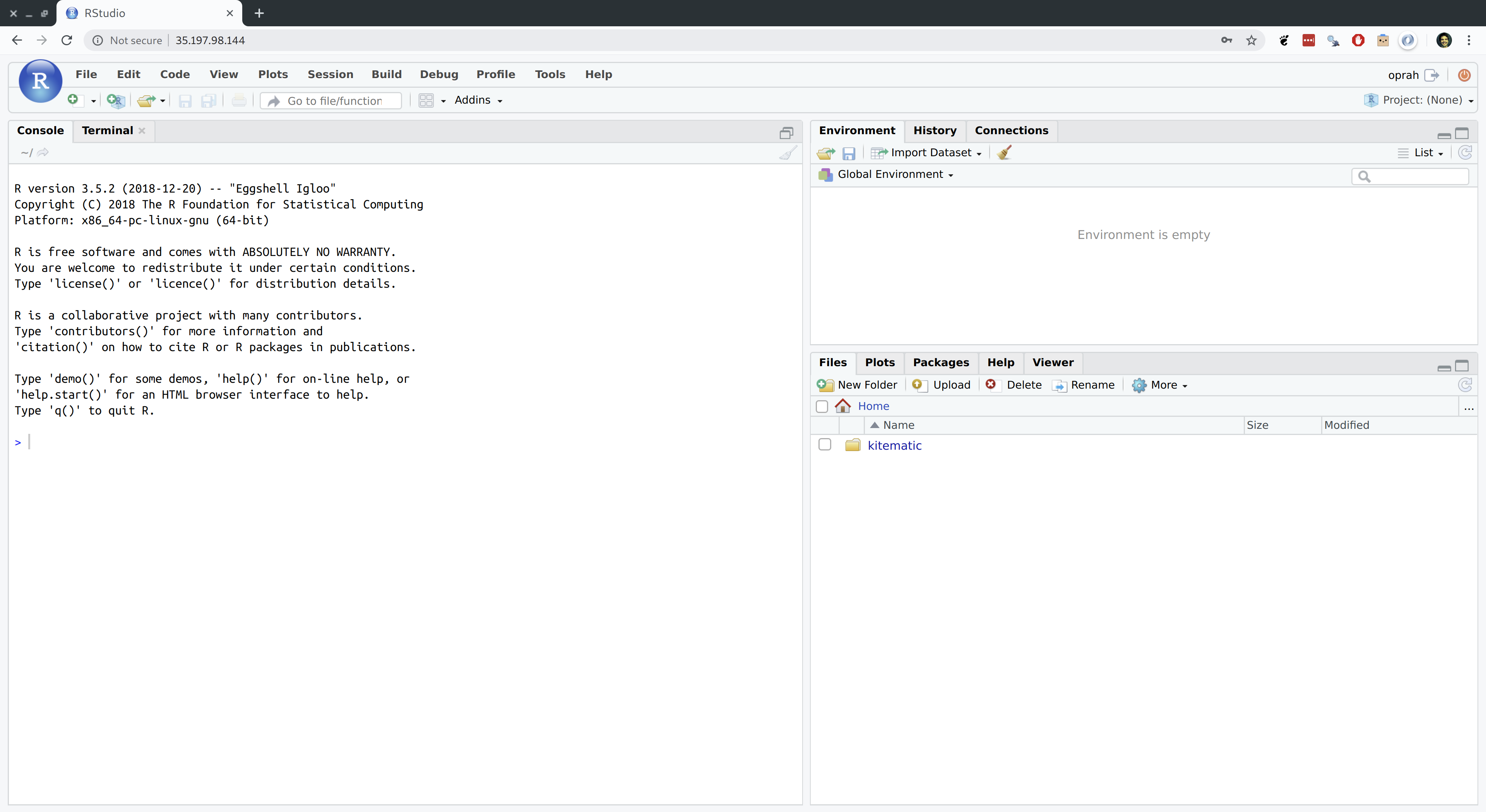
And that's really all you need. To log in, simply click on the external IP address. (Note: you do not need to add the 8787 port this time.) Just to prove that it worked, here's a screenshot of "Oprah" running RStudio Server on this VM.
It's also very easy to stop, (re)start, and delete a VM instance.
```{r vm_delete}
gce_vm_stop("new-vm") ## Stop the VM
# gce_vm_start("new-vm") ## If you wanted to restart
gce_vm_delete("new-vm") ## Delete the VM (optional)
```
## Cluster of VMs
**Note:** This section isn't working for Windows users at present. Follow along [here](https://github.com/cloudyr/googleComputeEngineR/issues/137) for a longer discussion of the problem (related to SSH keys) and, hopefully, a solution at some point.
At the risk of gross simplification, there are two approaches to "brute force" your way through a computationally-intensive problem.^[Of course, you can also combine a cluster of very power machines to get a *really* powerful system. That's what supercomputing services like the University of Oregon's [Talapas cluster](https://hpcf.uoregon.edu/content/talapas) provide, which is the subject of a later lecture.]
1. Use a single powerful machine that has a lot of memory and/or cores.
2. Use cluster of machines that, together, have a lot of memory/or and cores.
Thus far we've only explored approach no. 1. For this next example, I want to show you how to implement approach no. 2. In particular, I want to show you how to spin up a simple cluster of VMs that you can interact with directly from your *local* RStudio instance. Yes, you read that correctly.
I'll demonstrate the effectiveness of this approach by calling a very slightly modified version of the `slow_func()` function that we saw in previous lectures. Essentially, this function is just meant to emulate some computationally-intensive process by imposing an enforced wait at the end of every run (here: five seconds). It is also a classic case of of a function that can be sped up in parallel.
```{r slow_func}
## Emulate slow function
slow_func =
function(x = 1) {
x_sq = x^2
d = data.frame(value=x, value_squared=x_sq)
Sys.sleep(5)
return(d)
}
```
Okay, let's see how these GCE clusters work in practice. I'm going to walk you through several examples. The first example is going to keep things as simple as possible, to introduce you to the key concepts. We'll add complexity (although not too much) in the examples that follow thereafter.
#### Simple cluster
For this first cluster example, I'm going to spin up three "g1-small" VM instances. These are [preemptible](https://cloud.google.com/compute/docs/instances/preemptible) VMs that can each use 1 CPU during short bursts. So, not powerful machines by any stretch of the imagination. But they are very cheap to run and multiple g1-small instances be combined very easily to make a pretty powerful machine. You typically see these preemptible VMs used for quick, on-the-fly computation and then discarded.^[It is also possible to spin up preemptible versions of other, larger VMs using the `scheduling = list(preemptible = TRUE)` argument. We'll see an example of that shortly.]
First, we create (and start) three VMs using the `gce_vm_cluster()` convenience function. This will automatically take care of the SSH setup for us, as well as install the [rocker/r-parallel](https://hub.docker.com/r/rocker/r-parallel) Docker image on all the VMs by default. However, I'm going to install the (slightly smaller, quicker to install) [rocker/r-base](https://hub.docker.com/r/rocker/r-base/) image instead, since I'm only going to be using base R commands here. I also wanted to make you aware of the fact that you have options here.
```{r vms}
vms =
gce_vm_cluster(
vm_prefix = "simple-cluster", ## All VMs in our cluster will have this prefix
cluster_size = 3, ## How many VMs in our cluster?
docker_image = "rocker/r-base", ## Default is rocker/r-parallel
predefined_type = "g1-small" ## Cheap preemptible machine
)
```
And that's all it takes. We are ready to use our remote cluster. For this simple example, I'm going to loop `slow_func()` over the vector `1:15`. As a reference point, recall that the loop would take (15*5=) **75 seconds** to run sequentially.
To run the parallelised version on our simple 3-CPU cluster, I'm going to use the amazing [**future.apply**](https://github.com/HenrikBengtsson/future.apply) package that we covered in the [lecture on parallel programming](https://raw.githack.com/uo-ec607/lectures/master/12-parallel/12-parallel.html). As you can see, all I need to do is specify `plan(cluster)` and provide the location of the workers (here: the `vms` cluster that we just created). Everything else stays *exactly* the same, as if we were running the code on our local computer. It Just Works.TM
```{r future_cluster, dependson=vms}
# library(tictoc) ## For timing. Already loaded.
# library(future.apply) ## Already loaded.
plan(cluster, workers = as.cluster(vms))
tic()
future_cluster = future_lapply(1:15, slow_func)
toc()
```
And just look at that: **A three times speedup!** Of course, we could also have implemented this using `furrr::future_map()` instead of `future.apply::future_apply()`. (Feel free to prove this for yourself.) The key takeaways are that we were able to create a remote cluster on GCE with a few lines of code, and then interact with it directly from our local computer using future magic. Pretty sweet if you ask me.
Following good practice, let's stop and then delete this cluster of VMs so that we aren't billed for them.
```{r delete_cluster, dependson=vms, dependson=future_cluster}
## Shut down instances when finished
gce_vm_stop(vms)
gce_vm_delete(vms)
```
#### Cluster with nested parallelization
In the simple cluster example above, each VM only had 1 CPU. A natural next step is think about spinning up a cluster of VMs that have *multiple* cores. Why not spin up, say, $N$ machines with $K$ cores each to get an $N \times K$ times speed improvement? This is fairly easily done, although it requires a few extra tweaks. Our strategy here can be summarised as following two steps:
1. Parallelize across the remote VMs in our cluster
2. Parallelize within each VM, making sure we "chunk" the input data appropriately to avoid duplication.
Let's see how this works in practice with another example. We start off in exactly the same way as before, calling the `gce_vm_cluster()` function. The most material change in the below code chunk is that I'm now spinning up two "n1-standard-4" VM instances that each have four cores; i.e. eight cores in total.
> **Tip:** I'm limiting myself to an eight-core cluster here, because that's the limit imposed by the free GCP trial and I want everyone to follow along. You are more than welcome (encouraged even) to experiment with more ambitious clusters if you are not bound by the free trial.
Note that I'm also installing the (default) rocker/r-parallel Docker image on each VM, since this comes preloaded with the future functions that we'll need to paralleize operations on the VMs themselves. Finally, I'm going to use an optional `scheduling` argument that instructs GCE to use cheaper, preemptible instances. This is entirely up to you, of course, but I wanted to show you the option since preemptible instances are ideally suited for this type of problem.
```{r vms_nested}
vms_nested =
gce_vm_cluster(
vm_prefix = "nested-cluster",
cluster_size = 2,
#docker_image = "rocker/r-parallel", ## CHANGED: Use the (default) rocker/r-parallel Docker image
predefined_type = "n1-standard-4", ## CHANGED: Each VM has four CPUs
scheduling = list(preemptible = TRUE) ## OPTIONAL: Use cheaper, preemptible machines
)
```
Now comes part where we need to tweak our cluster setup. Nesting in the future framework is operationalised by defining a series of so-called [future "topologies"](https://cran.r-project.org/web/packages/future/vignettes/future-3-topologies.html). You can click on the previous link for more details, but the gist is that we define a nested plan of futures using the `plan(list(tweak(...), tweak(...)))` syntax. In this case, we are going to define two topology layers:
- **Topology 1.** The "outer" plan, which tells `future` to use the cluster of two remote VMs.
- **Topology 2.** The "inner" plan, which tells future to use all four cores on each VM via the `multicore` option.
```{r plan_nested, message=FALSE, dependson=vms_nested, results=FALSE, eval=FALSE}
plan(list(
## Topology 1: Use the cluster of remote VMs
tweak(cluster, workers = as.cluster(vms_nested)),
## Topology 2: Use all CPUs on each VM
tweak(multicore)
))
```
That wasn't too complicated, was it? We are now ready to use our cluster by feeding it a parallel function that can take advantage of the nested structure. Here is one potential implementation that seems like it should work. I haven't run it here, however, because there is something that we probably want to fix first. Can you guess what it is? (Try running the command yourself and then examining the output if you aren't sure.) The answer is underneath.
```{r, cache=FALSE, eval=FALSE}
## NOT RUN (Run it yourself to see why it yields the wrong answer)
## Outer future_lapply() loop over the two VMS
future_lapply(seq_along(vms_nested), function(v) {
## Inner future_lapply() loop: 16 asynchronous iterations of our slow function
future_lapply(1:16, slow_func)
})
```
The problem with the above code is that it will duplicate the exact same 16 iterations on *each* VM, instead of splitting up the job efficiently between them. What we want to do, then, is split the input data into distinct "chunks" for each VM to work on separately. There are various ways to do this chunking, but here's an option that I've borrowed from [StackOverflow](https://stackoverflow.com/a/16275428). I like this function because it uses only base R functions and is robust to complications like unequal chunk lengths and different input types (e.g. factors vs numeric).
```{r chunk_func}
chunk_func = function(x, n) split(x, cut(seq_along(x), n, labels = FALSE))
## Examples (try them yourself)
# chunk_func(1:8, 2)
# chunk_func(1:5, 3)
# chunk_func(as.factor(LETTERS[1:5]), 2)
```
Okay, now we're really ready to make full use our cluster. For this example, I'll even go ahead and run 40 iterations of our `slow_func()` function in total. Note that this would take 200 seconds to run sequentially. Based on the total number of cores available to us in this cluster, we would we hope to drop this computation time to around 25 seconds (i.e. an **8 times speedup**) by running everything in parallel. I've commented the code quite explicitly, so please read carefully to see what's happening. In words, though: first we parallelize over the two VMs; then we chunk the input data so that each VM works on a distinct part of problem; and finally we feed the chunked data to our `slow_func` function where it is run in parallel on each VM.
```{r future_nested_cluster_noeval, dependson=vms_nested, eval=FALSE}
## Input data (vector to be iterated over by our function)
input_data = 1:40
tic()
## Run the function in (nested) parallel on our cluster
future_nested_cluster =
## Outer future_lapply() loop over the two VMS
future_lapply(seq_along(vms_nested), function(v) {
## Split the input data into distinct chunks for each VM
input_chunk = chunk_func(input_data, length(vms_nested))[[v]]
## Inner future_lapply() loop within each of the VMs
future_lapply(input_chunk, slow_func)
})
toc()
```
```{r future_nested_cluster, dependson=vms_nested, message=FALSE, echo=FALSE}
## NOTE: This chunk simply repeats the previous ones, but actually *evaluates*
## them. Why do this? Because keeping the plan() and the future_lapply() calls
## together avoids problems with Rmd caching missteps. Obviously we'll set
## echo=FALSE to avoid printing things out twice in the knitted document.
plan(list(
## Topology 1: Use the cluster of remote VMs
tweak(cluster, workers = as.cluster(vms_nested)),
## Topology 2: Use all CPUs on each VM
tweak(multicore)
))
## Input data (vector to be iterated over by our function)
input_data = 1:40
tic()
## Run the function in (nested) parallel on our cluster
future_nested_cluster =
## Outer future_lapply() loop over the three VMS
future_lapply(seq_along(vms_nested), function(v) {
## Split the input data into distinct chunks for each VM
input_chunk = chunk_func(input_data, length(vms_nested))[[v]]
## Inner future_lapply() loop within each of the VMs
future_lapply(input_chunk, slow_func)
})
toc()
```
And it worked! There's a little bit of overhead, but we are very close to the maximum theoretical speedup. Note that this overhead time would increase if we were transferring large amounts of data around the cluster --- which, again future will take care of automatically for us --- but the same basic principles would apply.
**Bottom line:** You can create can create a mini supercomputer up in the cloud using only a few lines of code, and then interact with it directly from your local R environment. Honestly, what's not to like?
Normally, I would remind you to shut down your VM instances now. But first, let's quickly using them again for one last example.
#### One final example
The final example that I'm going to show you is a slight adaptation of the nested cluster that we just covered.^[Indeed, we're going to be using the same two VMs. These should still be running in the background, unless you've taken a long time to get to this next section. Just spin them up again if you run into problems.] This time we're going to install and use an additional R package on our remote VMs that didn't come pre-installed on the "r-parallel" Docker image. (The package in question is going to be [**data.table**](https://raw.githack.com/uo-ec607/lectures/master/05-datatable/05-datatable.html), but that's not really the point of the exercise.) I wanted to cover this kind of scenario because a) it's very likely that you'll want to do something similar if you start using remote clusters regularly, and b) the commands for doing so aren't obvious if you're not used to R scripting on Docker containers. The good news is that it's pretty easy once you've seen an example and that everything can be done through `plan()`. Let's proceed.
The [`Rscript`](https://raw.githack.com/uo-ec607/lectures/master/03-shell/03-shell.html#rscript) shell command is probably the most common way to install additional R packages on a Docker container at load time. The slight complication here is that we we need this to happen on each of the remote VMs in our cluster. That's what the `rscript = c(...)` line below is doing; it's launching `Rscript` in each Docker container. Next we feed it the actual command, i.e. `Rscript -e install.packages(PACKAGE)`. This looks a little abstruse here, because it has to go through the `rscript_args = c(...)` argument, but hopefully you get the idea.
```{r plan_nested_DT, dependson=vms_nested, message=FALSE, results=FALSE, eval=FALSE}
plan(list(
## Topology 1: Use the cluster of remote VMs
tweak(cluster,
workers = as.cluster(
vms_nested,
## Launch Rscript inside the r-parallel Docker containers on each VM
rscript = c(
"docker", "run", "--net=host", "rocker/r-parallel",
"Rscript"
),
## Install the data.table package on the R instances running in the containers
rscript_args = c("-e", shQuote("install.packages('data.table')"))
)
),
## Topology 2: Use all the CPUs on each VM
tweak(multicore)
))
```
(Note: I've hidden the output from the above code chunk, because takes up quite of vertical space with all of the installation messages, etc. You should see messages detailing **data.table**'s installation progress across each of your VMs if you run this code on your own computer.)
Let's prove to ourselves that the installation of **data.table** worked by running a very slightly modified version of our earlier code. This time we'll use `data.table::rbindList()` to coerce the resulting list objects from each `future_lapply()` call into a data table. Note that we'll need to do this twice: once for our inner loop(s) and once for the outer loop.
```{r future_nested_cluster_DT_noeval, dependson=vms_nested, eval=FALSE}
## Same as earlier, but this time binding the results into a data.table with
## data.table::rbindlist()
## Run the function in (nested) parallel on our cluster
future_nested_cluster_DT =
## Bind into a data.table
data.table::rbindlist(
## Outer future_lapply() loop over the two VMs
future_lapply(seq_along(vms_nested), function(v) {
## Split the input data into distinct chunks for each VM
input_chunk = chunk_func(input_data, length(vms_nested))[[v]]
## Inner future_lapply() loop within each of the VMs
data.table::rbindlist(future_lapply(input_chunk, slow_func))
})
)
## Show that it worked
future_nested_cluster_DT
```
```{r future_nested_cluster_DT, dependson=vms_nested, message=FALSE, echo=FALSE}
## NOTE: This chunk simply repeats the previous ones, but actually *evaluates*
## them. Why do this? Because keeping the plan() and the future_lapply() calls
## together avoids problems with Rmd caching missteps. Obviously we'll set
## echo=FALSE to avoid printing things out twice in the knitted document.
plan(list(
## Topology 1: Use the cluster of remote VMs
tweak(cluster,
workers = as.cluster(
vms_nested,
## Launch Rscript inside the r-parallel Docker containers on each VM
rscript = c(
"docker", "run", "--net=host", "rocker/r-parallel",
"Rscript"
),
## Install the data.table package on the R instances running in the containers
rscript_args = c("-e", shQuote("install.packages('data.table')"))
)
),
## Topology 2: Use all the CPUs on each VM
tweak(multicore)
))
## Same as earlier, but this time binding the results into a data.table with
## data.table::rbindlist()
## Run the function in (nested) parallel on our cluster
future_nested_cluster_DT =
## Bind into a data.table
data.table::rbindlist(
## Outer future_lapply() loop over the three VMs
future_lapply(seq_along(vms_nested), function(v) {
## Split the input data into distinct chunks for each VM
input_chunk = chunk_func(input_data, length(vms_nested))[[v]]
## Inner future_lapply() loop within each of the VMs
data.table::rbindlist(future_lapply(input_chunk, slow_func))
})
)
## Show that it worked
future_nested_cluster_DT
```
And would you just look at that. It worked like a charm. We're so awesome.
These, being preemptible VMs, will automatically be deleted within 24 hours. But there's no need to have them sitting around incurring charges now that we're done with them.
```{r delete_nested_cluster, dependson=future_nested_cluster}
## shutdown instances when finished
gce_vm_stop(vms_nested)
gce_vm_delete(vms_nested)
```
## Other topics and further resources
The **googleComputeEngineR** package offers a lot more functionality than I can cover here. However, I wanted to briefly mention the fact that GCE offers GPU instances that are production-ready for training hardcore deep learning models. In my view, this is one of the most exciting developments of cloud-based computation services, as it puts the infrastructure necessary for advanced machine learning in the hands of just about everyone. See Mark's [introductory GPU tutorial](https://cloudyr.github.io/googleComputeEngineR/articles/gpu.html) on the **googleComputeEngineR** website. *Note:* These GPU instances are not available during the GCP free trial period, although users can always upgrade their account if they want.
Here are some further resources that you may wish to consult.
- The [googleComputeEngineR website](https://cloudyr.github.io/googleComputeEngineR/index.html) is very good, providing lots of helpful examples.
- Thinking about other cloud platforms with transferable ideas, [Davis Vaughan](https://blog.davisvaughan.com/) provides a concise [AWS example](https://davisvaughan.github.io/furrr/articles/advanced-furrr-remote-connections.html) using the `furrr` package (which treads a similar path to our nested `future_lapply()` example). [Andrew Heiss](https://www.andrewheiss.com/) has a very lucid [blog tutorial on his Digital Ocean setup](https://www.andrewheiss.com/blog/2018/07/30/disposable-supercomputer-future/) for those who want to try going that route.