Chapter 2 What is Structural Modeling?
In this chapter, I explain what structural modeling is and how it can be useful to economists. A nice treatment of this topic is Reiss and Wolak (2007), which I borrow some materials from.
In the simplest sense, structural modeling (or, interchangeably, structural econometrics) is a combination of economic and statistical models. Structural models are used in every empirical field of economics: from dynamic stochastic general equilibrium (DSGE) models in macroeconomics to models of firm decision-making in industrial organization to individual choice models in labor.
More formally, a structural model is an attempt to estimate policy-invariant fundamental parameters, also known as structural parameters. The parameter estimates can then be used to predict outcomes in a counterfactual setting. Typically, structural parameters are those parameters which enter an agent’s utility function or production function (and cost function). Structural models may also incorporate constraints faced by the agent(s), strategic behavior among competing agents, or other aspects of economic theory such as moral hazard in a principal-agent scenario. Once the econometrician knows the preferences, production technology, and constraints of the agent(s), she can predict how the agent(s) will behave in a new scenario for which there is no existing data.
Structural models are especially useful in settings where an experiment cannot be undertaken. In this case, one must specify how the unobservables are related to the observables, because this relationship cannot be ignored without the randomization that occurs in an experiment.
2.1 Advantages and Disadvantages of Structural Models
Many economists shy away from structural models because using them forces the researcher to make strong assumptions about how the world works. In essence a structural model is a researcher’s view of the world. To the extent that the model includes unreasonable or unrealistic assumptions, one must discount any results derived from the model.
Another reason some economists dislike structural models is because they can be difficult to estimate. Structural models typically are nonlinear (even if they are linear-in-parameters) and estimation typically requires using maximum likelihood or method of moments estimation as opposed to linear regression techniques.
The main advantage of using a structural model is that it can be a powerful tool for predicting the effects of potential policies. If one knows the data generating process (DGP), then one does not need to do any statistical estimation. Structural modeling is an attempt to estimate the parameters of the DGP. Once the DGP is known, one can use it to simulate what might happen under counterfactual scenarios.
2.2 A simple structural model
One toy example that often appears in introductory econometrics textbooks is the effect of education on earnings. Typically, the textbook presents an equation like this: \[\log\left(wage_{i}\right)=\beta_0 + \beta_{1}educ_{i}+\varepsilon_{i}\] where \(wage_i\) is the individual’s wage as an adult, and \(educ_i\) is the individual’s years of completed education (e.g. 12 for a high school graduate, 16 for a college graduate, etc.).
2.3 Other examples
- Tuition subsidy (Keane and Wolpin (1997))
- IO demand estimation (BLP, etc.)
- IO production function estimation (Collard-Wexler papers)
- IO entry games (…)
- Trade markups (De Loecker, Eeckhout, and Unger (2018))
- Development (…)
- Migration (Kennan and Walker (2011))
- Regional demand and commuting flows (Monte, Redding, and Rossi-Hansberg (2018))
You can label chapter and section titles using {#label} after them, e.g., we can reference Chapter 2. If you do not manually label them, there will be automatic labels anyway, e.g., Chapter 4.
Figures and tables with captions will be placed in figure and table environments, respectively.
par(mar = c(4, 4, .1, .1))
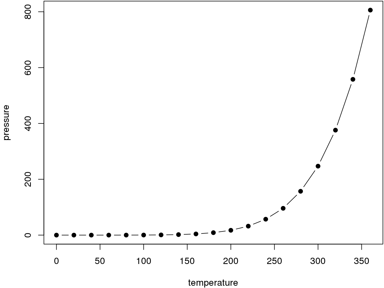
plot(pressure, type = 'b', pch = 19)
Figure 2.1: Here is a nice figure!
Reference a figure by its code chunk label with the fig: prefix, e.g., see Figure 2.1. Similarly, you can reference tables generated from knitr::kable(), e.g., see Table 2.1.
knitr::kable(
  head(iris, 20), caption = 'Here is a nice table!',
  booktabs = TRUE
)| Sepal.Length | Sepal.Width | Petal.Length | Petal.Width | Species |
|---|---|---|---|---|
| 5.1 | 3.5 | 1.4 | 0.2 | setosa |
| 4.9 | 3.0 | 1.4 | 0.2 | setosa |
| 4.7 | 3.2 | 1.3 | 0.2 | setosa |
| 4.6 | 3.1 | 1.5 | 0.2 | setosa |
| 5.0 | 3.6 | 1.4 | 0.2 | setosa |
| 5.4 | 3.9 | 1.7 | 0.4 | setosa |
| 4.6 | 3.4 | 1.4 | 0.3 | setosa |
| 5.0 | 3.4 | 1.5 | 0.2 | setosa |
| 4.4 | 2.9 | 1.4 | 0.2 | setosa |
| 4.9 | 3.1 | 1.5 | 0.1 | setosa |
| 5.4 | 3.7 | 1.5 | 0.2 | setosa |
| 4.8 | 3.4 | 1.6 | 0.2 | setosa |
| 4.8 | 3.0 | 1.4 | 0.1 | setosa |
| 4.3 | 3.0 | 1.1 | 0.1 | setosa |
| 5.8 | 4.0 | 1.2 | 0.2 | setosa |
| 5.7 | 4.4 | 1.5 | 0.4 | setosa |
| 5.4 | 3.9 | 1.3 | 0.4 | setosa |
| 5.1 | 3.5 | 1.4 | 0.3 | setosa |
| 5.7 | 3.8 | 1.7 | 0.3 | setosa |
| 5.1 | 3.8 | 1.5 | 0.3 | setosa |