Bayesian Model Averaging of (a)symmetric IRT Models in Small Samples

Fabio Setti & Leah Feuerstahler

Fordham University

Estimation and Sample Size in IRT

The more item parameters are added to the model, the more flexible the item response functions (IRFs).

However, the additional parameters of the 3PL and 4PL tend to require large sample sizes (\(N \geq 1000\)) to be stably estimated.

We will be focusing on 1PL and 2PL models

Maximum Likelihood

1PL models seem to be stably estimable with sample sizes as low as \(N = 100\) (Finch & French, 2019).

2PL models seems to require a sample size of \(N = 200\) or more (Drasgow, 1989; Liu & Yang, 2018).

Markov Chain Monte Carlo

1PL models showed good coverage when \(N = 100\) and generally outperformed maximum likelihood (Finch & French, 2019).

2PL models with hierarchical priors perform reasonably well even when \(N = 100\) (König et al., 2020).

Simple Asymmetric IRT Models

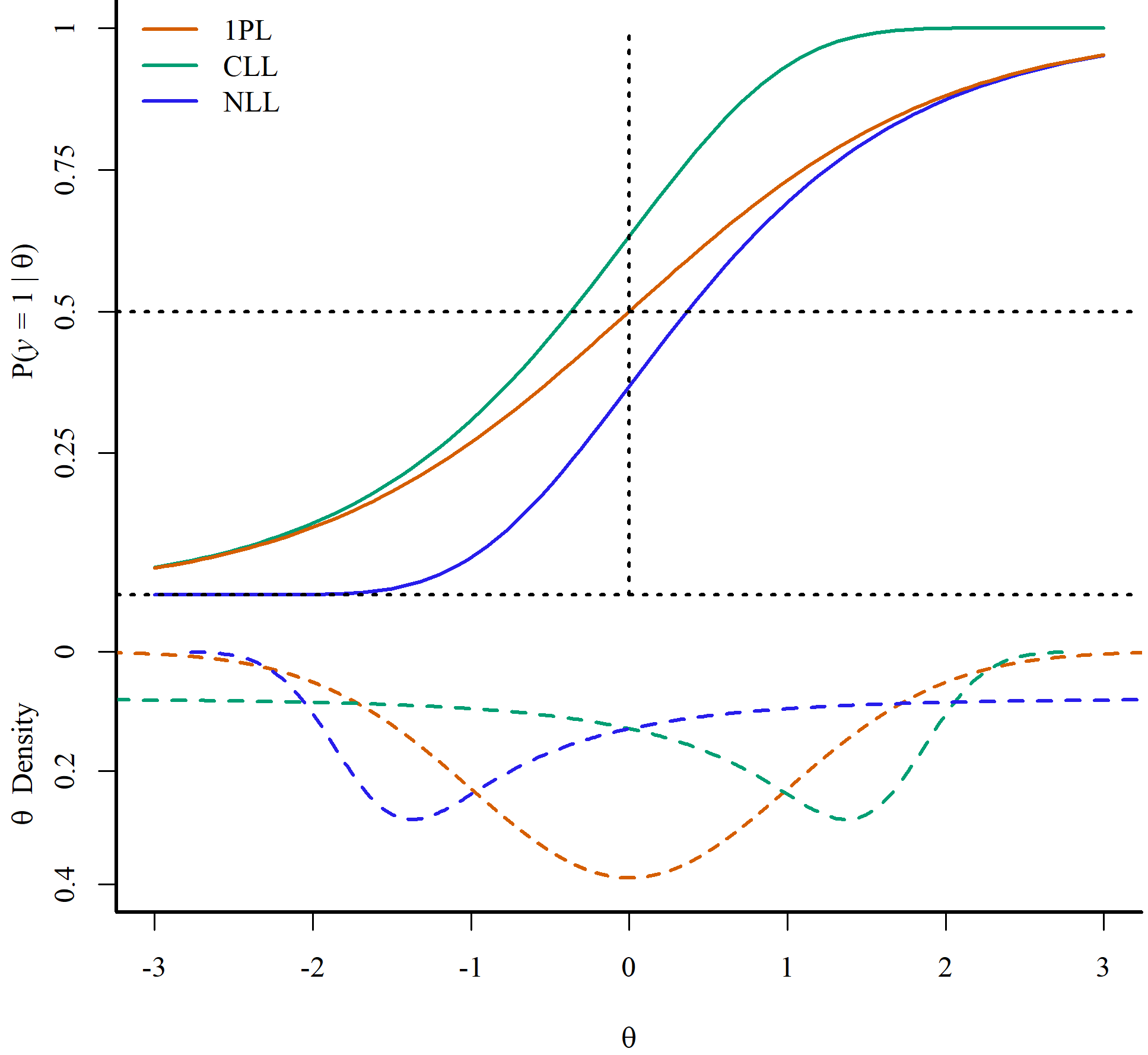
Most asymmetric models include asymmetry parameters that are hard to estimate in small sample sizes (e.g., Gonçalves et al., 2023; Lee & Bolt, 2018; Verkuilen & Johnson, 2024) Two recently proposed asymmetric IRT models (Shim et al., 2023a, 2023b) may help address this issue:

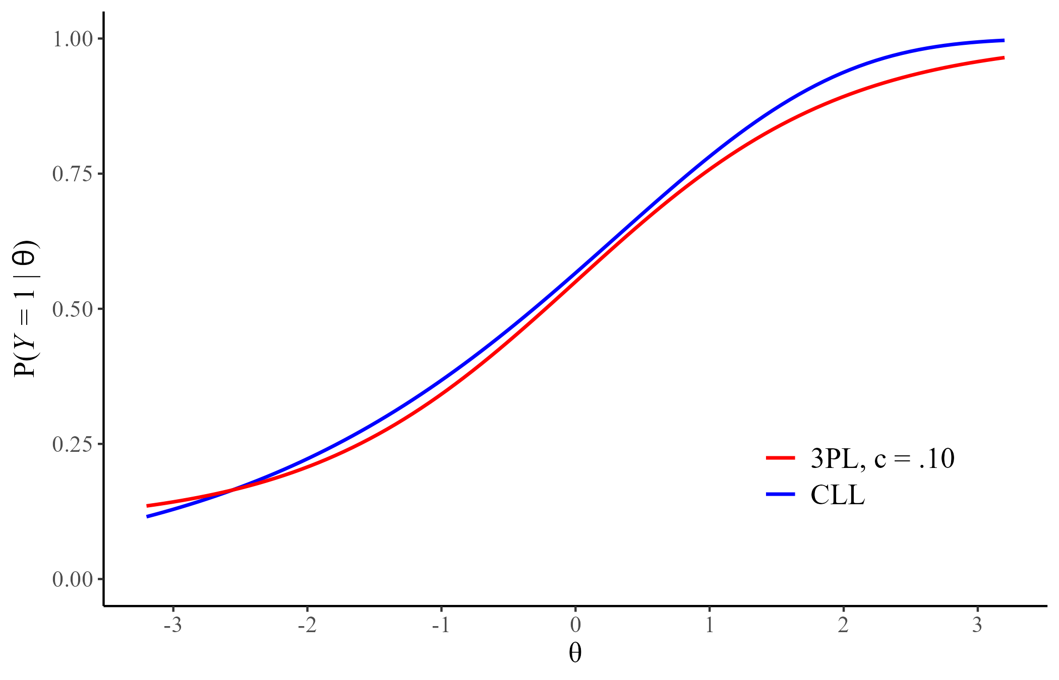
Complementary Log-Log (CLL)

\[ P(Y = 1| \theta) = 1 - \exp[-\exp[a(\theta - b)]]\]

Negative Log-Log (NLL)

\[ P(Y = 1| \theta) = \exp[-\exp[-a(\theta - b)]]\]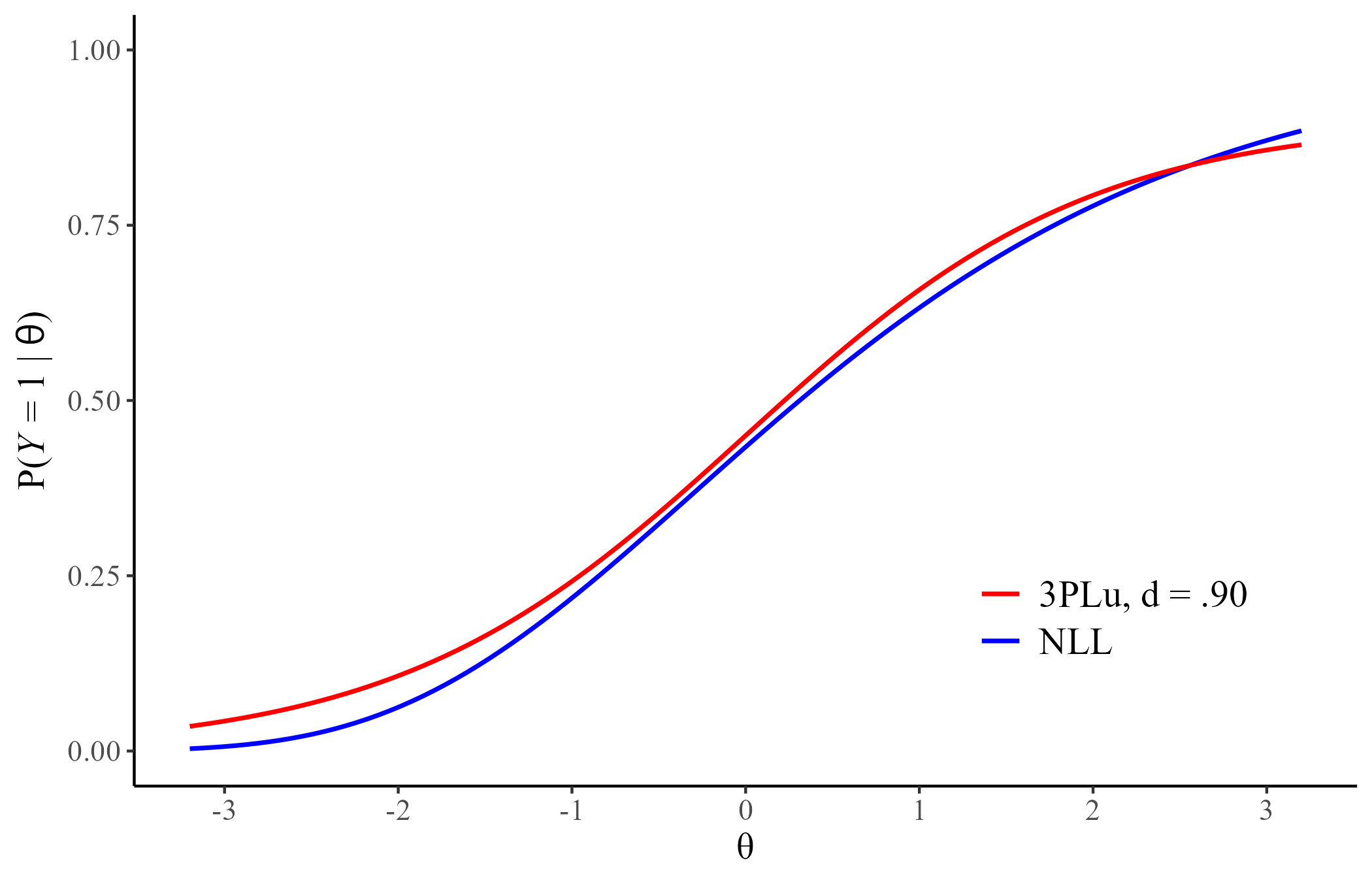

What to do about Small Sample Sizes?

Although the NLL and CLL may approximate more complex models, complex IRFs remain hard to approximate in small sample sizes (\(N \leq 250\)) with a single model.

Can we do better with Bayesian model averaging (BMA)?

Model averaging takes into account model uncertainty by weighting a set of candidate models according to their relative plausibility.

BMA weights are based on a leave-one-out cross validation approximation (Vehtari et al., 2017). This provides a fit measure for each data point.

Calculating model weights:

• Test level weights

• Item level weights?

Two type of weights (Yao et al., 2018):

• BMA weights with Bayesian bootstrapping (BMA+)

• Stacking weights

Averaging Predicted Probability of Keyed Responses

Theoretical quantiles

estimate \(P(Y = 1|\theta)\) by averaging along a common \(\theta\) continuum. Assumes a common \(\theta\) scale across models.

Empirical quantiles

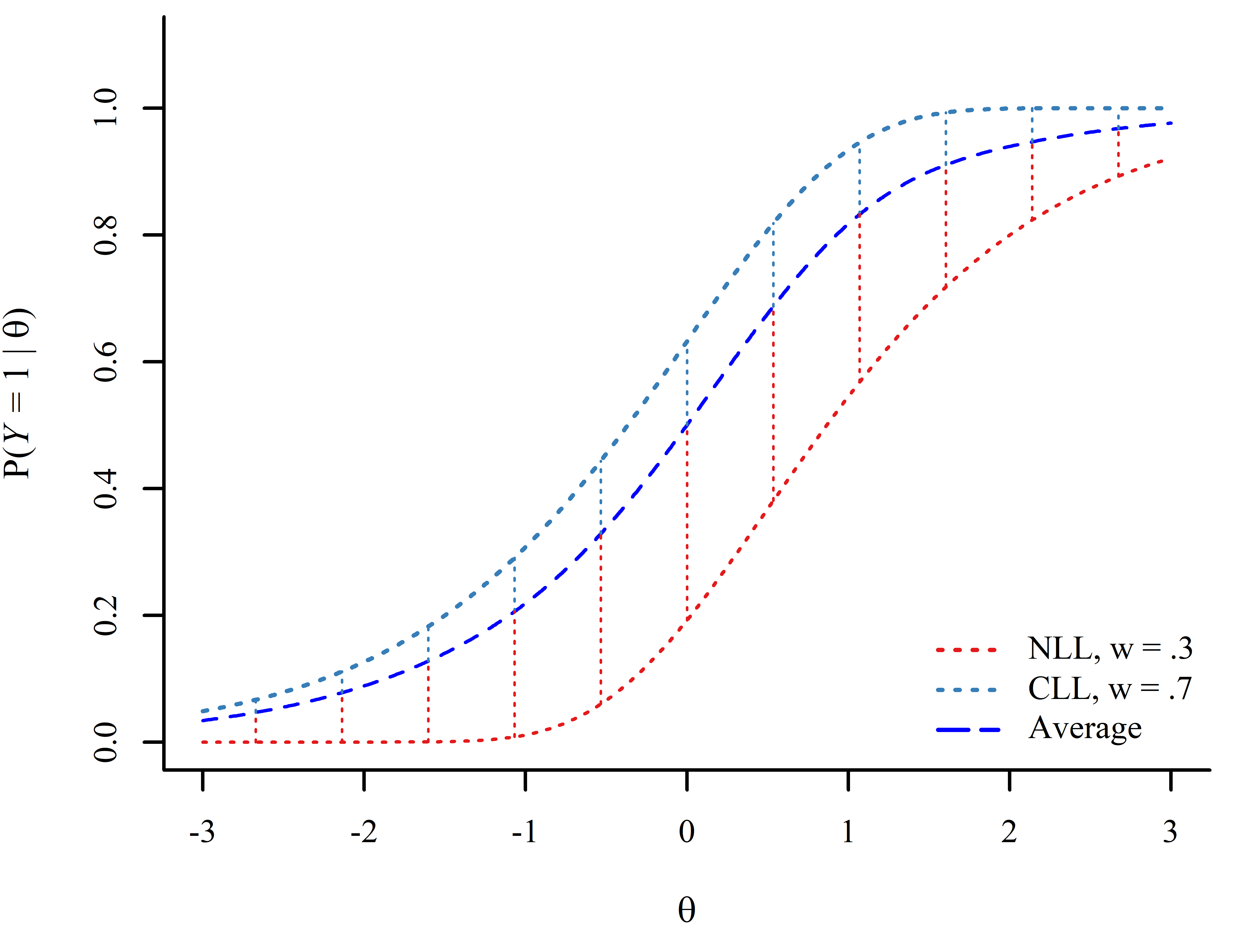
estimate \(P(Y = 1|\theta)\) by averaging along a common empirical \(\theta\) continuum. Can accommodate different \(\theta\) scales.

Empirical Example

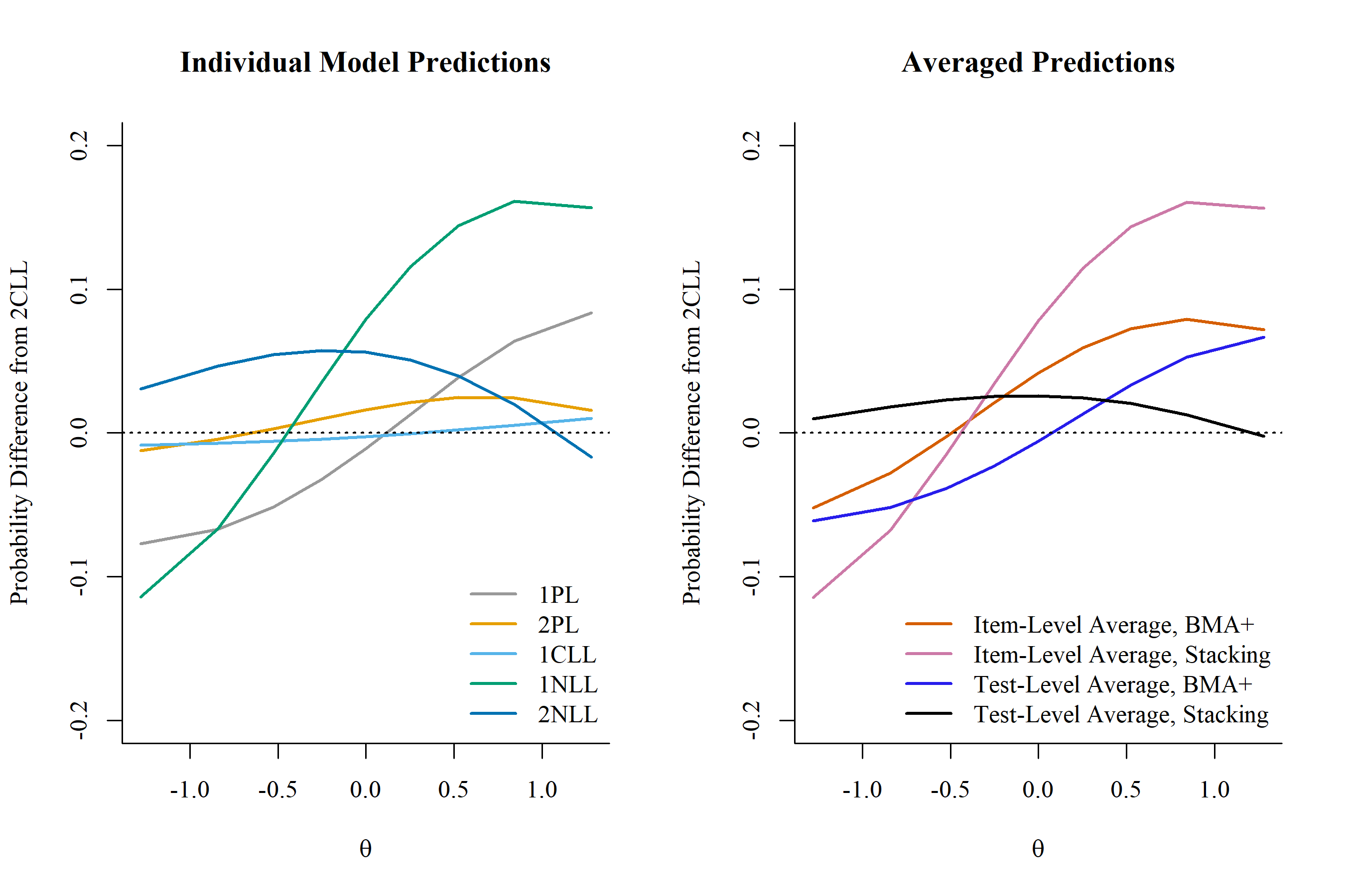
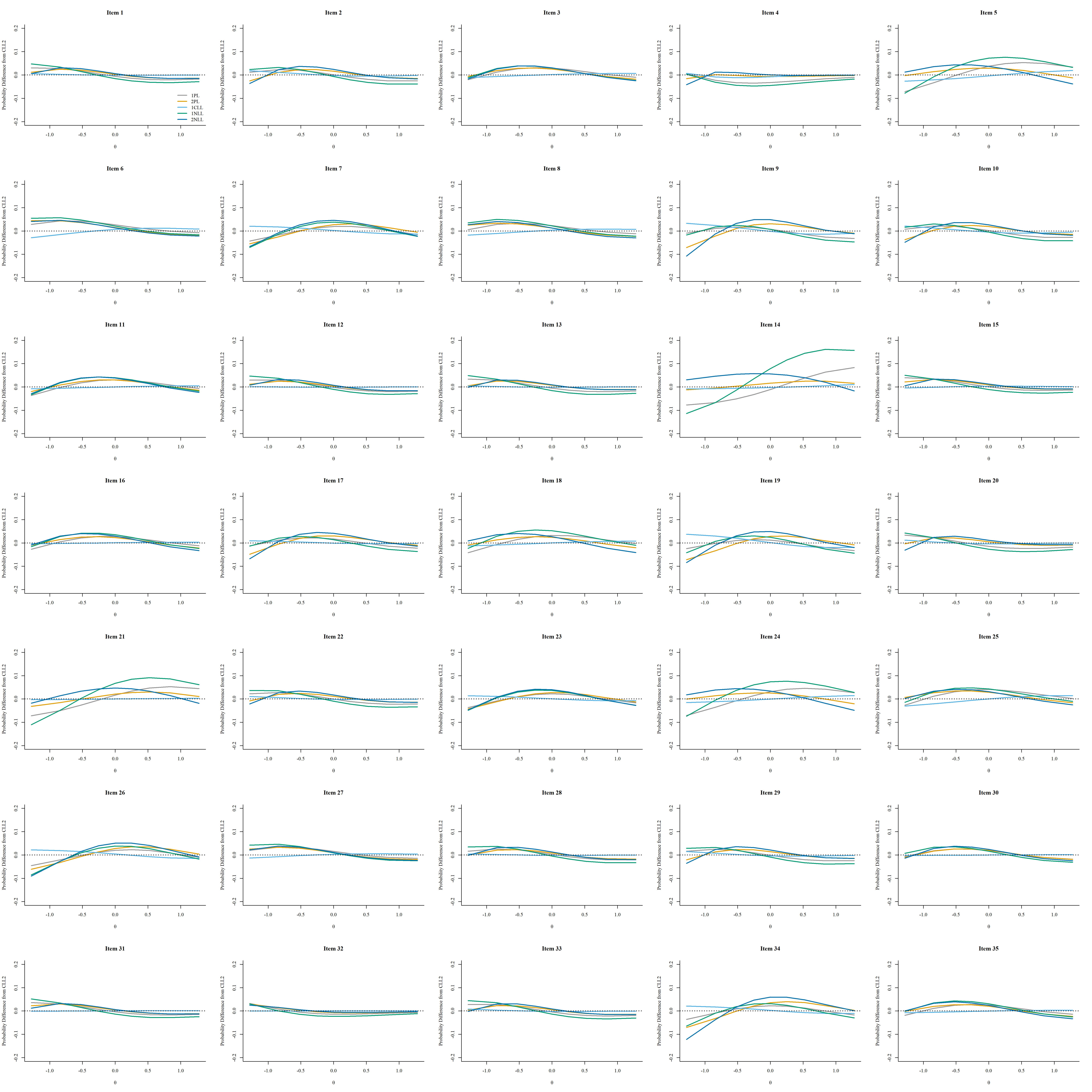
We fit the 1PL, 2PL, 1CLL, 2CLL, 1NLL, 2NLL with the brms package (Bürkner, 2017) to the Bond’s Logical Operations Test (BLOT; Bond & Fox, 2007) dataset from the PsychTools package (Revelle, 2024), which includes 150 participants and 35 items.

Predictions for Item 14

Simulation

Most data generating condition purposely introduced some type of model misspecification. There were 4 data generating conditions:

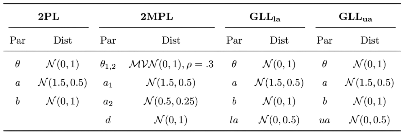
2PL: \(\frac{\exp[a(\theta - b)]}{1 + \exp[a(\theta - b)]}\)

2MPL: \(\frac{1}{1 +\exp[-(a_{1}\theta_{1} + a_{2}\theta_{2} + d)]}\)

GLL_la and GLL_ua (Zhang et al., 2022)

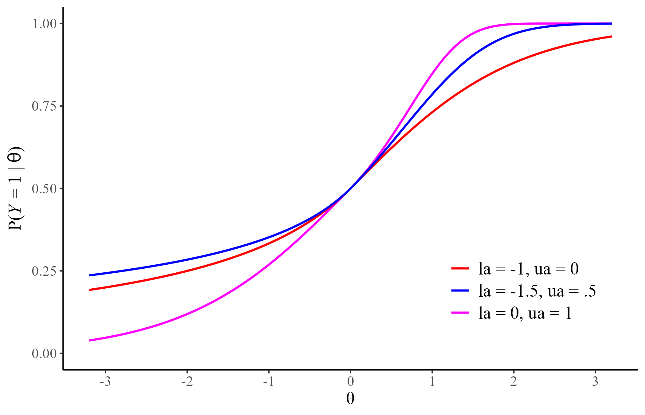
• 4 data-generating models (2PL, 2MPL, GLL_la, GLL_ua)
• 2 sample sizes (N = 100, 250)
• 2 test lengths (I = 10, 20)
• 100 replications (R)
• 9 quantiles (q = .10,…,.90)

We will compare the performance of model selection (MS), test averaging (TA), item averaging (IA), and kernel smoothing IRT (KS):

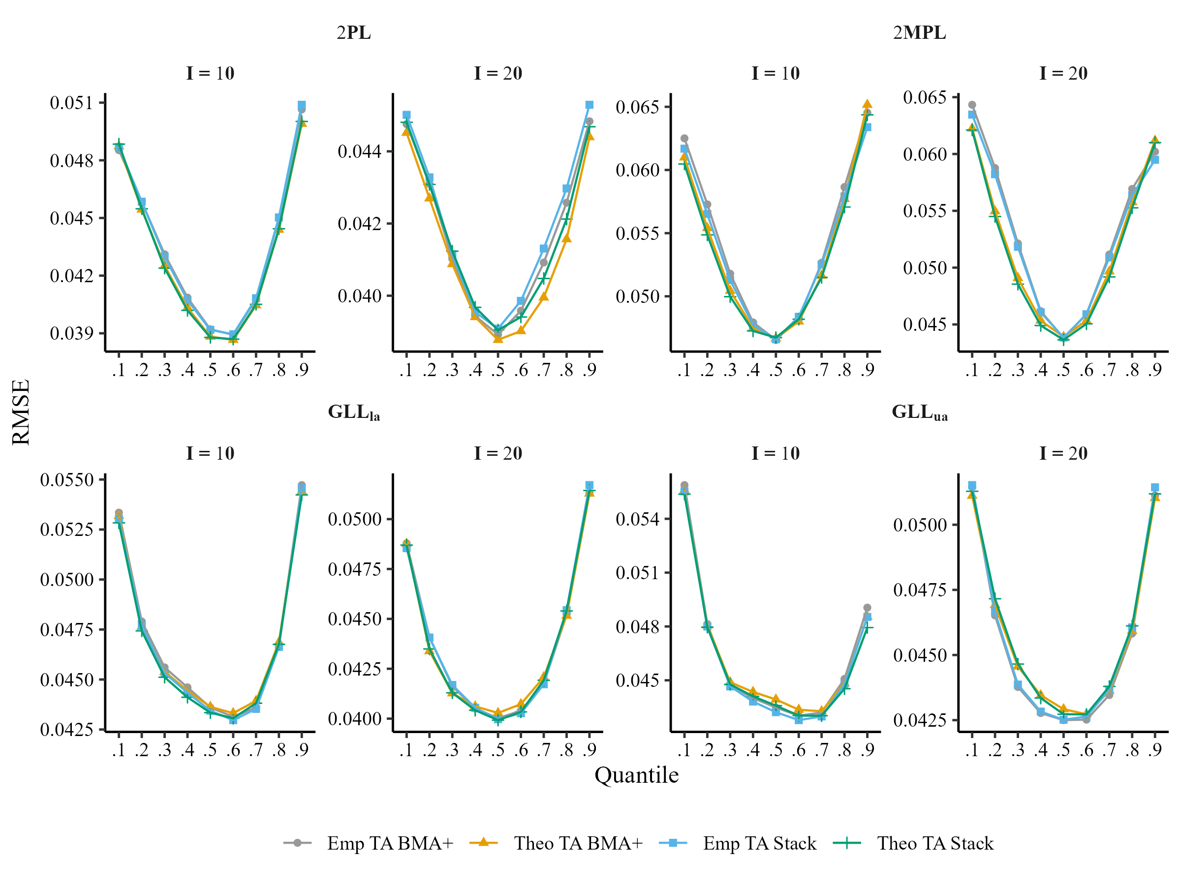
\[RMSE_{q} = \sqrt{\frac{1}{100}\sum_{r=1}^{100}\frac{1}{I}\sum_{i = 1}^{I}[P_r(y_{in} = 1|\theta_{q}) - \hat{P}_r(y_{in} = 1|\tilde{\theta}_{q})]^{2}}\]

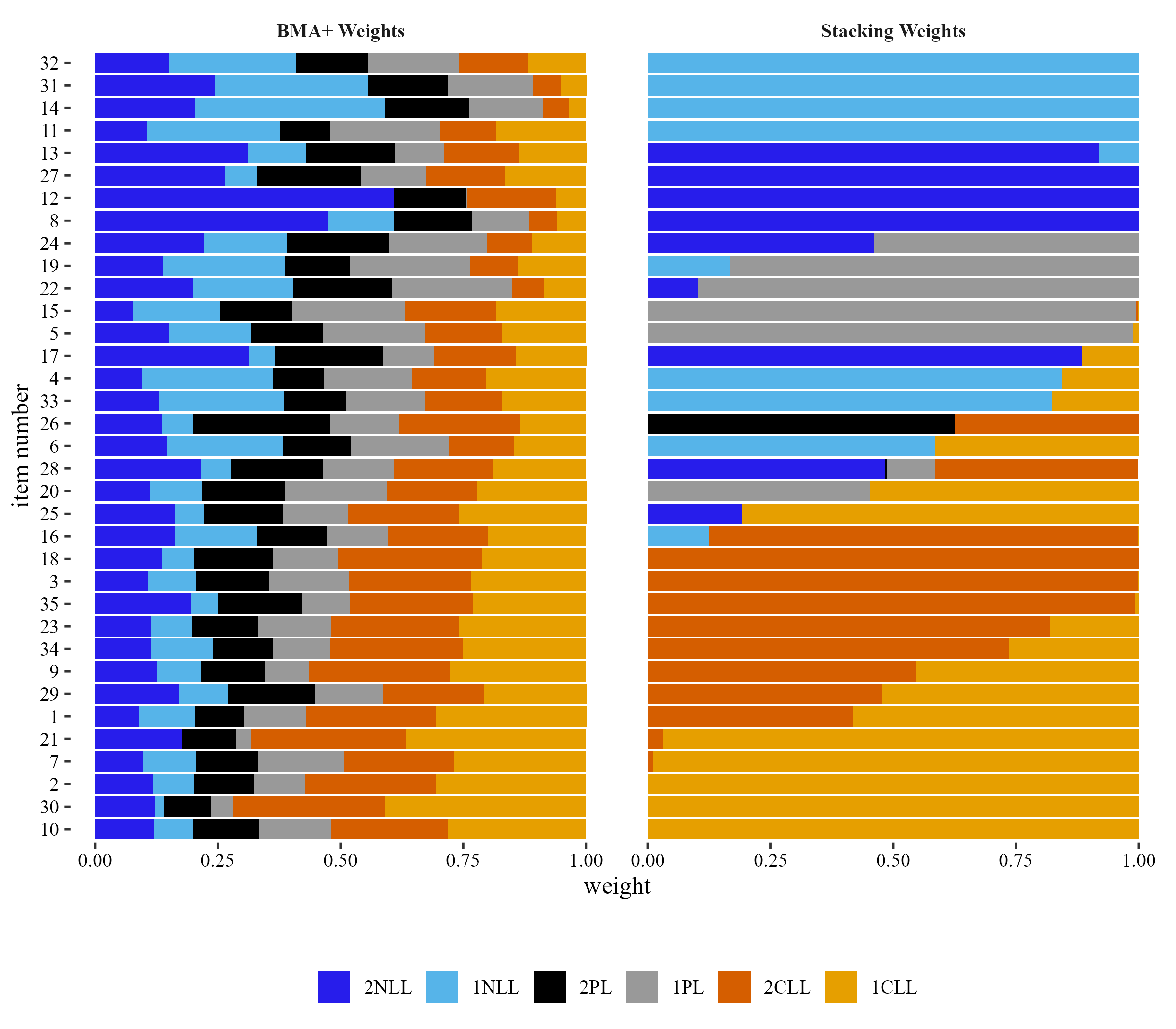
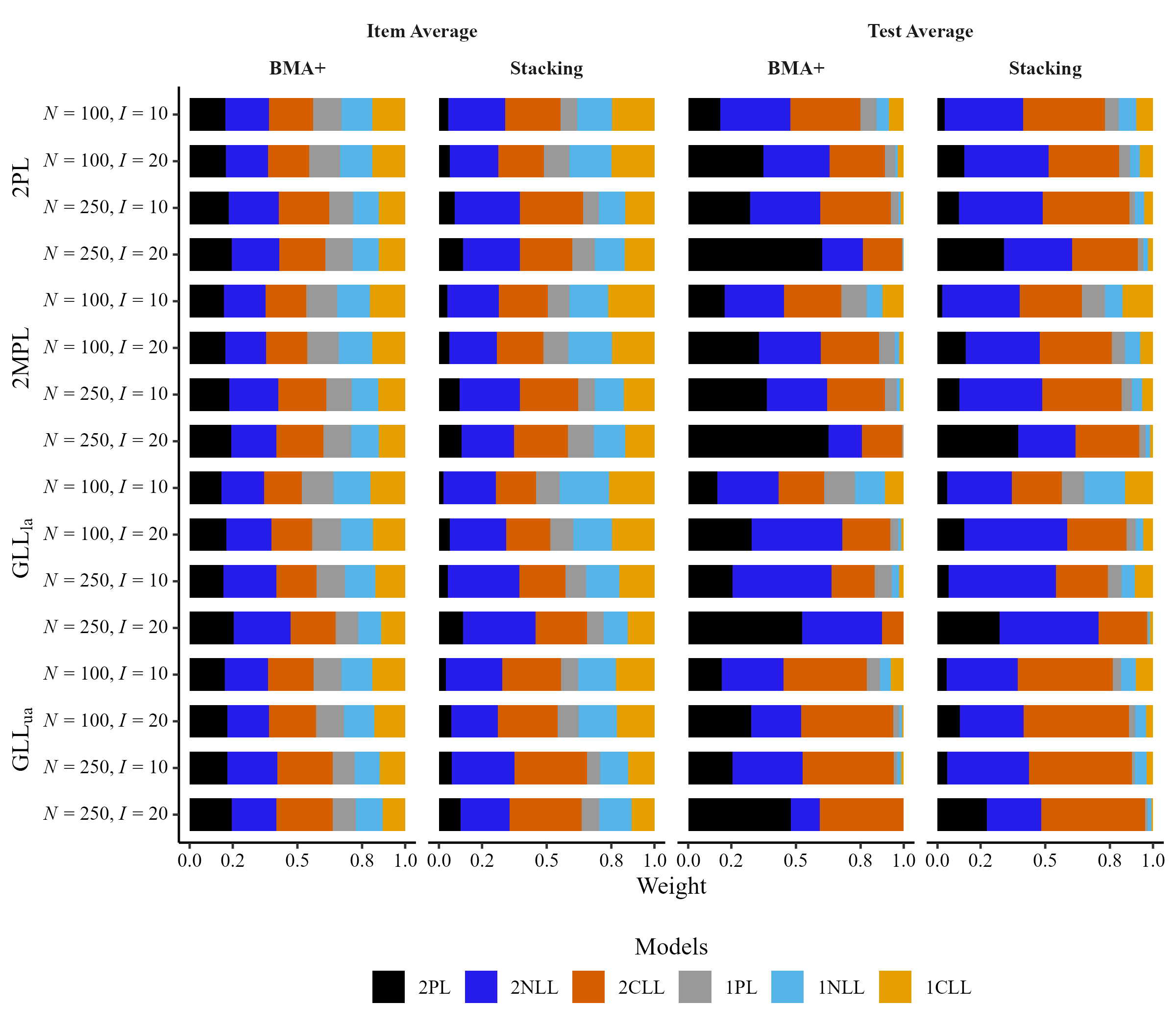
Distribution of Test and Item Weights

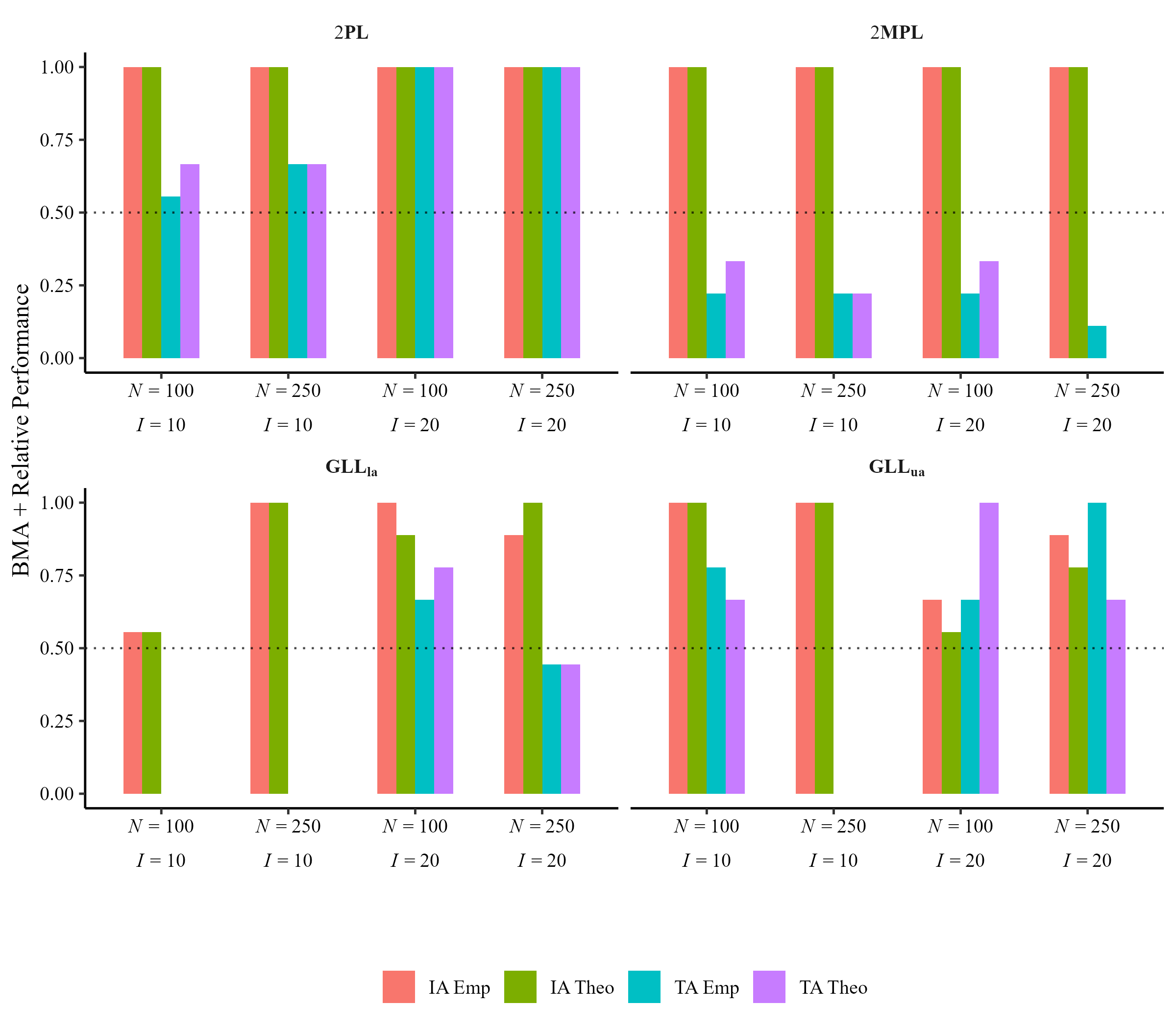
Performance of BMA+ Over Stacking Weights

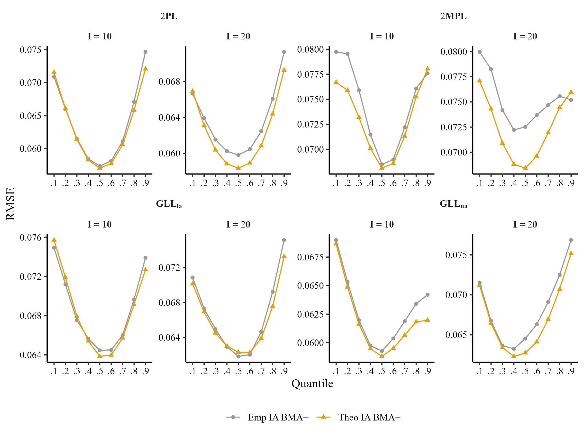
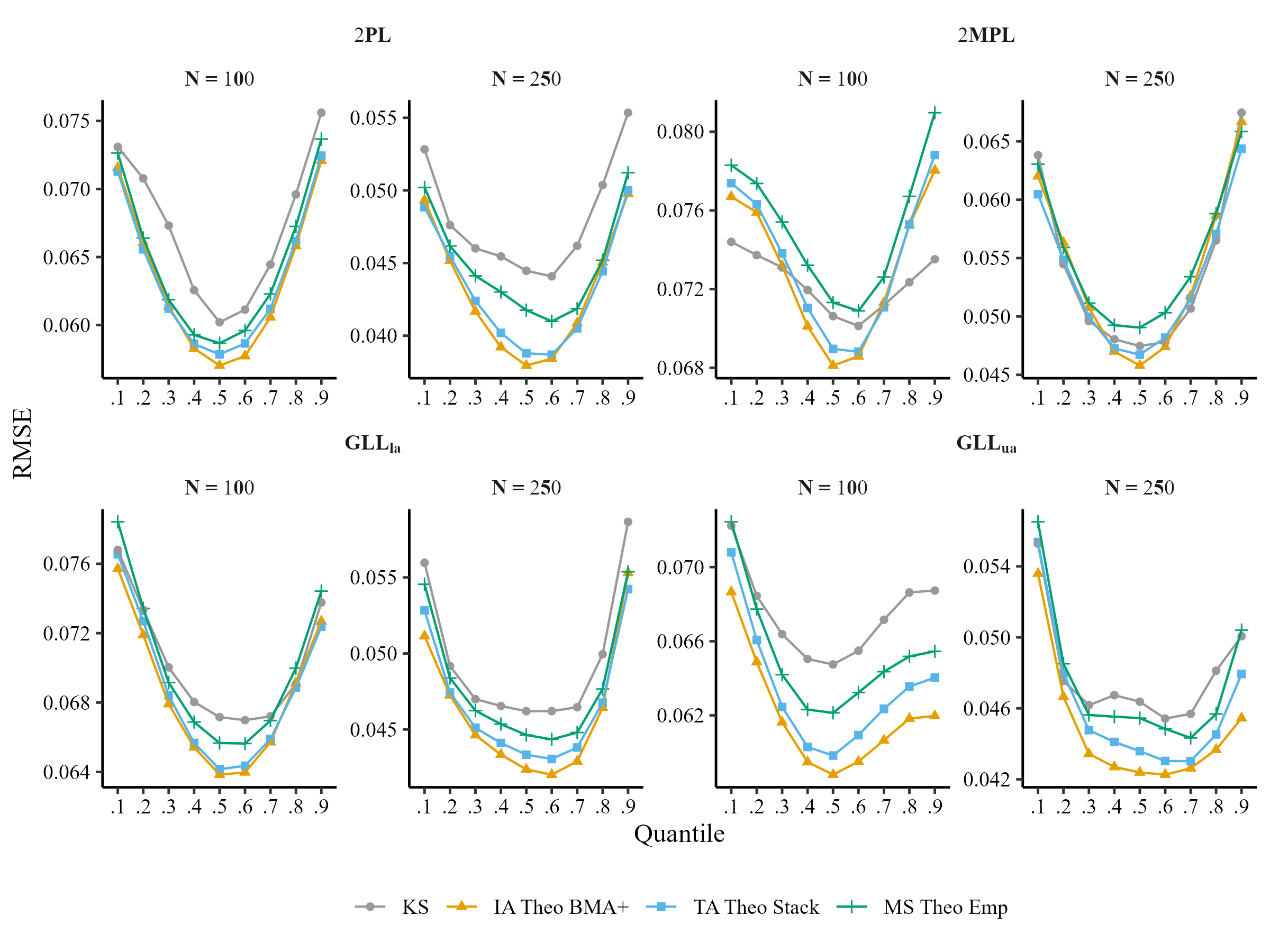
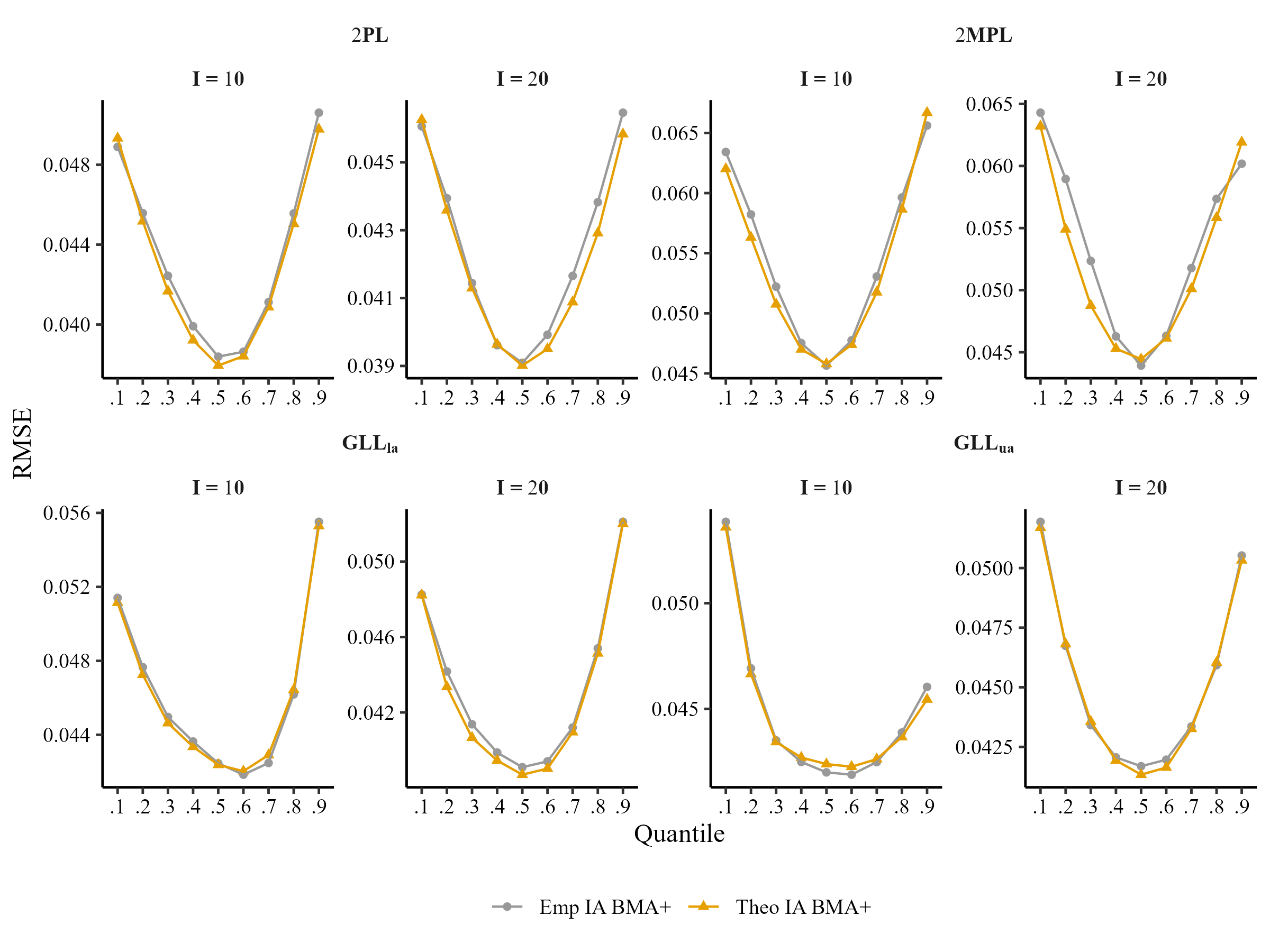
Comparison of Item Averaging at Theoretical and Empirical Quantiles (N = 100)

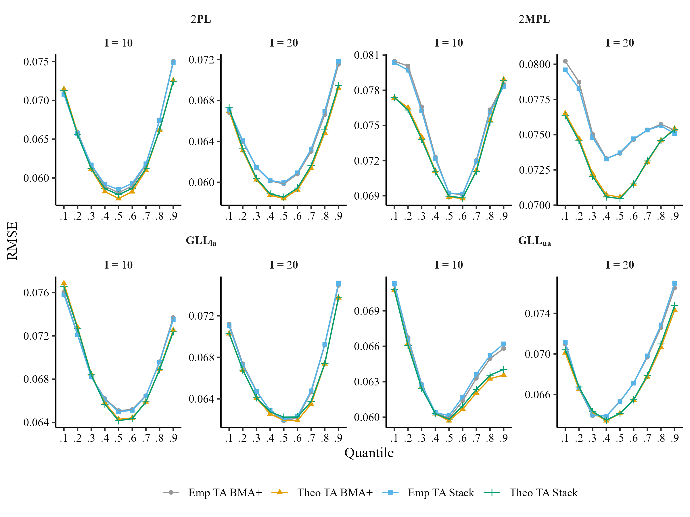
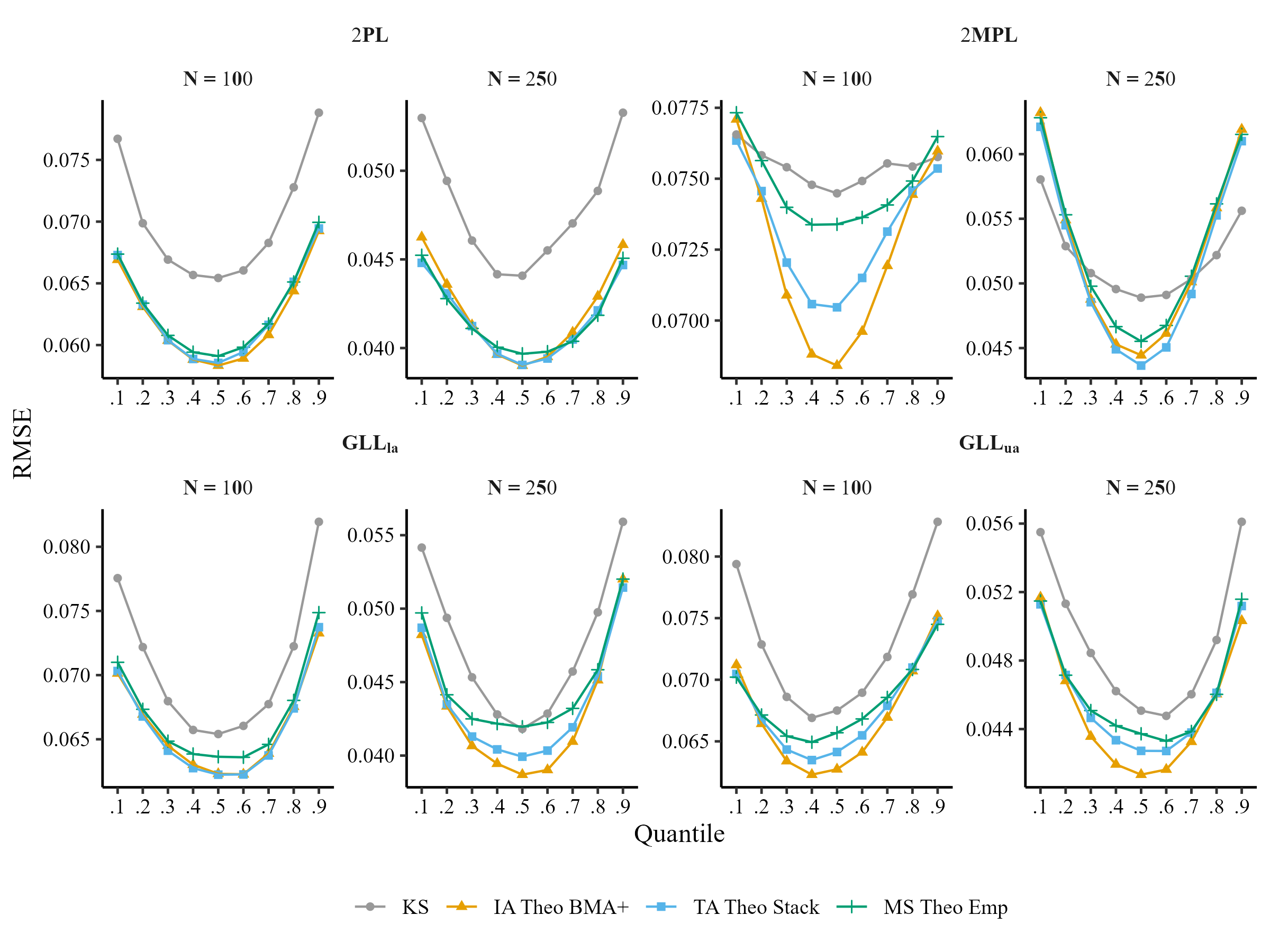
Comparison of Test Averaging at Theoretical and Empirical Quantiles (N = 100)

Comparison of Averaging Methods, Model selection (MS), Kernel Smoothing (KS) for I = 10

Comparison of Averaging Methods, Model selection (MS), Kernel Smoothing (KS) for I = 20

Summary of Results

• Item weights may provide useful insight into individual item behavior.

• Either item weights or test weights can provide a stable method of detecting and estimating asymmetry in small sample sizes.

• Item level averaging, followed by test level averaging, consistently offered better IRF recovery.

• BMA+ weights showed better performance for IA, while stacking weights and BMA + weights performed similarly in the case of TA.

Acknowledgement & Contacts

Acknowledgements

• My advisor: Leah Feuerstahler (leah@fordham.edu)

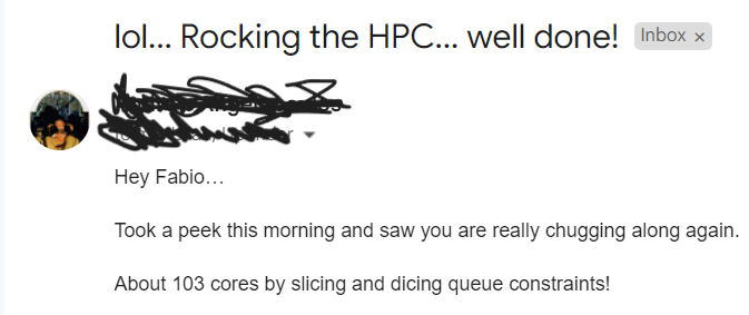
• Fordham’s High Performance Computing team, especially Andrew Angelopoulos (aangelopoulos@fordham.edu)

Contact and slides link

• my email: fsetti@fordham.edu

Slides QR code:

References

Bond, T. G., & Fox, C. M. (2007). Applying the Rasch Model: Fundamental Measurement in the Human Sciences, Second Edition (2nd ed.). Psychology Press. https://doi.org/10.4324/9781410614575

Bürkner, P.-C. (2017). Brms: An R package for bayesian multilevel models using stan. Journal of Statistical Software, 80, 1–28. https://doi.org/10.18637/jss.v080.i01

Drasgow, F. (1989). An Evaluation of Marginal Maximum Likelihood Estimation for the Two-Parameter Logistic Model. Applied Psychological Measurement, 13(1), 77–90. https://doi.org/10.1177/014662168901300108

Finch, H., & French, B. F. (2019). A comparison of estimation techniques for IRT models with small samples. Applied Measurement in Education, 32(2), 77–96. https://doi.org/10.1080/08957347.2019.1577243

Gonçalves, F. B., Venturelli S. L., J., & Loschi, R. H. (2023). Flexible Bayesian modelling in dichotomous item response theory using mixtures of skewed item curves. British Journal of Mathematical and Statistical Psychology, 76(1), 69–86. https://doi.org/10.1111/bmsp.12282

König, C., Spoden, C., & Frey, A. (2020). An Optimized Bayesian Hierarchical Two-Parameter Logistic Model for Small-Sample Item Calibration. Applied Psychological Measurement, 44(4), 311–326. https://doi.org/10.1177/0146621619893786

Lee, S., & Bolt, D. M. (2018). Asymmetric item characteristic curves and item complexity: Insights from simulation and real data analyses. Psychometrika, 83(2), 453–475. https://doi.org/10.1007/s11336-017-9586-5

Liu, Y., & Yang, J. S. (2018). Interval Estimation of Latent Variable Scores in Item Response Theory. Journal of Educational and Behavioral Statistics, 43(3), 259–285. https://doi.org/10.3102/1076998617732764

Revelle, W. (2024). psychTools: Tools to Accompany the ’psych’ Package for Psychological Research (Version 2.4.3) [Computer software]. https://cran.r-project.org/web/packages/psychTools/index.html

Shim, H., Bonifay, W., & Wiedermann, W. (2023a). Parsimonious asymmetric item response theory modeling with the complementary log-log link. Behavior Research Methods, 55(1), 200–219. https://doi.org/10.3758/s13428-022-01824-5

Shim, H., Bonifay, W., & Wiedermann, W. (2023b). Parsimonious item response theory modeling with the negative log-log link: The role of inflection point shift. Behavior Research Methods. https://doi.org/10.3758/s13428-023-02189-z

Vehtari, A., Gelman, A., & Gabry, J. (2017). Practical bayesian model evaluation using leave-one-out cross-validation and WAIC. Statistics and Computing, 27(5), 1413–1432. https://doi.org/10.1007/s11222-016-9696-4

Verkuilen, J., & Johnson, P. J. (2024). Gumbel-Reverse Gumbel (GRG) Model: A New Asymmetric IRT Model for Binary Data. In M. Wiberg, J.-S. Kim, H. Hwang, H. Wu, & T. Sweet (Eds.), Quantitative Psychology (pp. 165–175). Springer Nature Switzerland. https://doi.org/10.1007/978-3-031-55548-0_16

Yao, Y., Vehtari, A., Simpson, D., & Gelman, A. (2018). Using stacking to average bayesian predictive distributions (with discussion). Bayesian Analysis, 13(3), 917–1007. https://doi.org/10.1214/17-BA1091

Zhang, J., Zhang, Y.-Y., Tao, J., & Chen, M.-H. (2022). Bayesian item response theory models with flexible generalized logit links. Applied Psychological Measurement, 46(5), 382–405. https://doi.org/10.1177/01466216221089343

Appendix

Model Priors

Model estimation used the partial pooling approach in the estimation of model parameters (i.e., random intercepts/slopes)

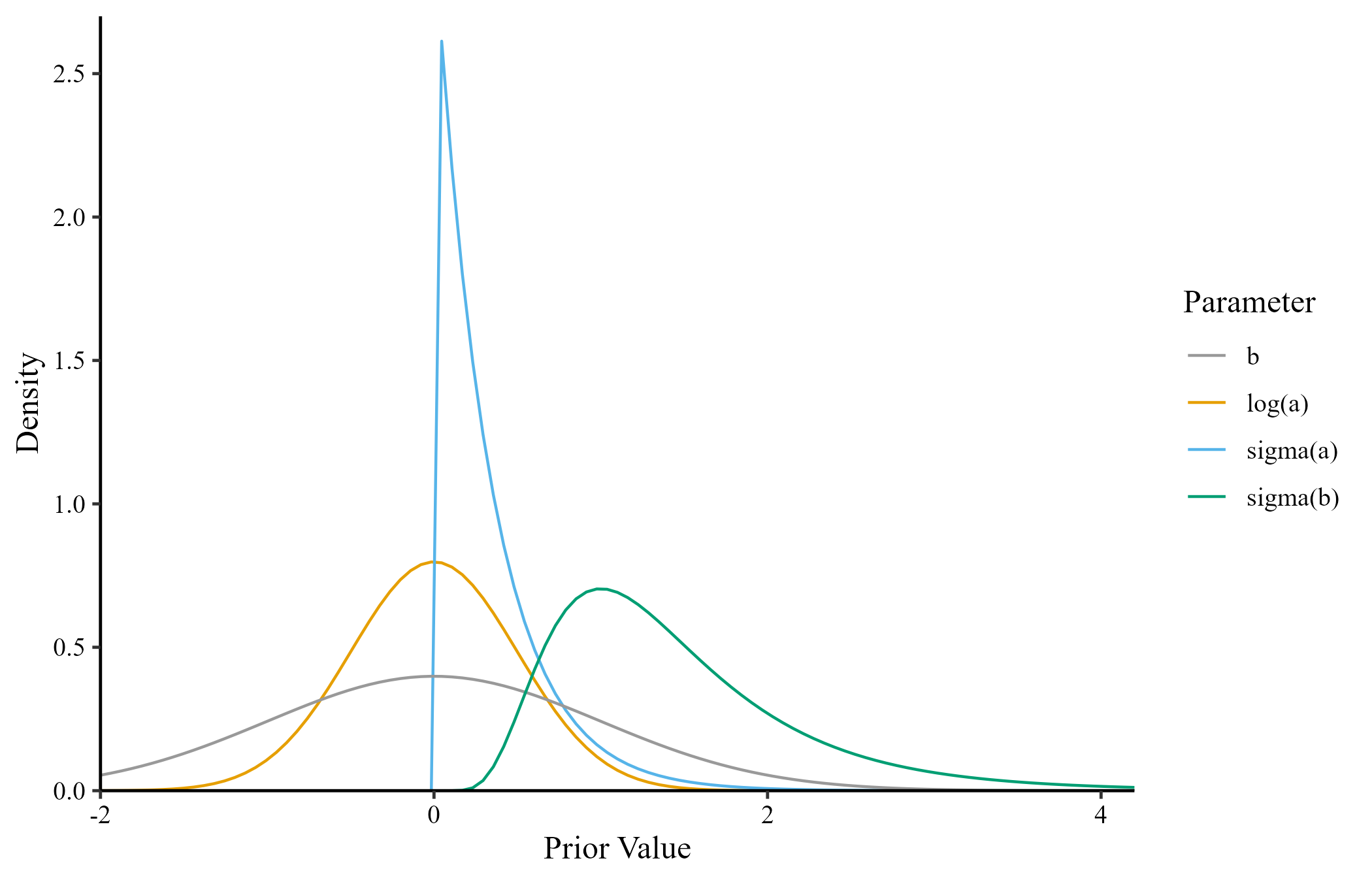
\(log(\bar{a}) = N(0, .5)\)

\(\sigma_{log(\bar{a})} = \mathrm{Exponential}(3)\)

\(\bar{b} = N(0, 1)\)

\(\sigma_{\bar{b}} = \mathrm{Lognormal}(.25, .5)\)

\(\bar{\theta} = 0\)

\(\sigma_\bar{\theta} = 1\)

IRF Averaging Scheme

1. Posterior distributions of parameters: The MCMC sampler provides \(N\) (6000 in this simulation) draws for each model parameter.

↓

2. Posterior distributions of \(P(Y = 1|\theta_q)\): The predicted probability of a keyed response is calculated at a set of empirical or theoretical quantiles , \(P(Y = 1|\theta_q)\), for all models across all MCMC draws.

↓

3. Model weights: A weight (stacking or BMA+) is calculated for each model.

↓

4. Averaged distribution of \(P(Y = 1|\theta_q)\): sample from each model distribution estimated in step 2 in proportion to model weight.

All BLOT items Predictions

Parameter Generating Distributions for Simulation

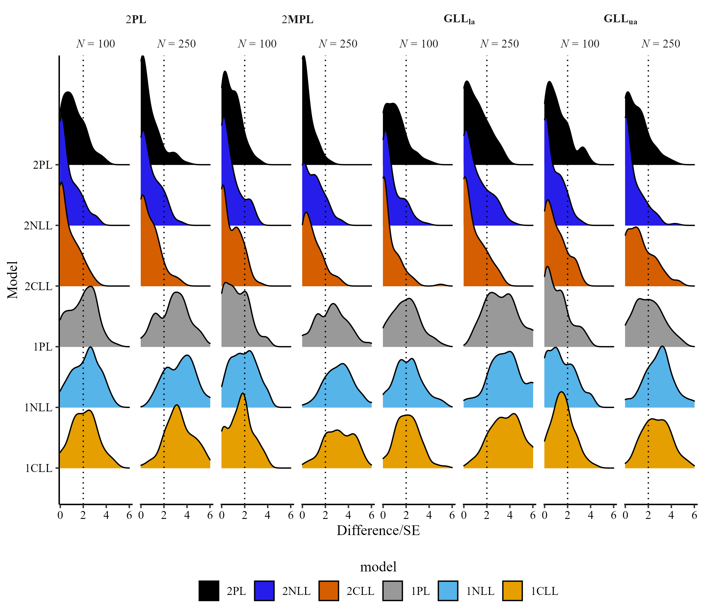
LOO diffrence/SE for I = 10

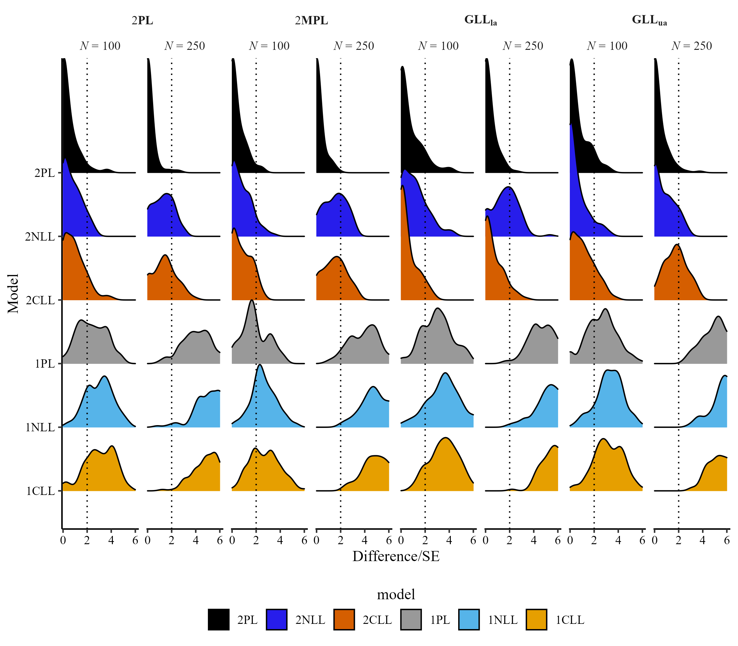
LOO diffrence/SE for I = 20

Comparison of Item Averaging at Theoretical and Empirical Quantiles (N = 250)

Comparison of Test Averaging at Theoretical and Empirical Quantiles (N = 250)