Measuring Forecasting Proficiency: An Item Response Theory Approach
Psychometrics
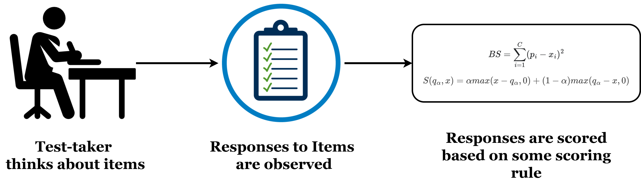
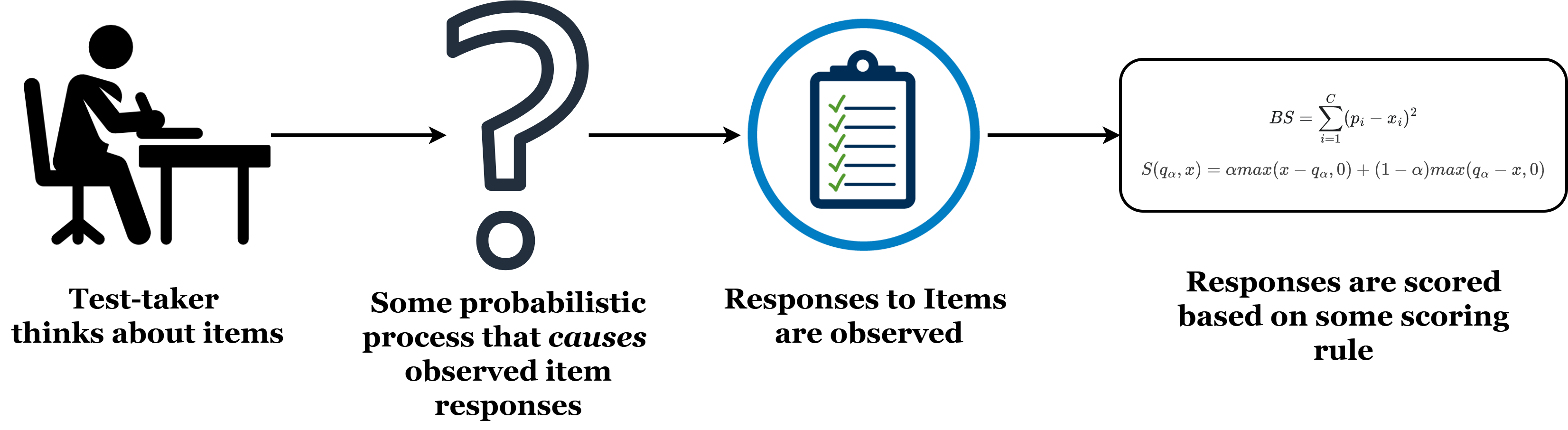
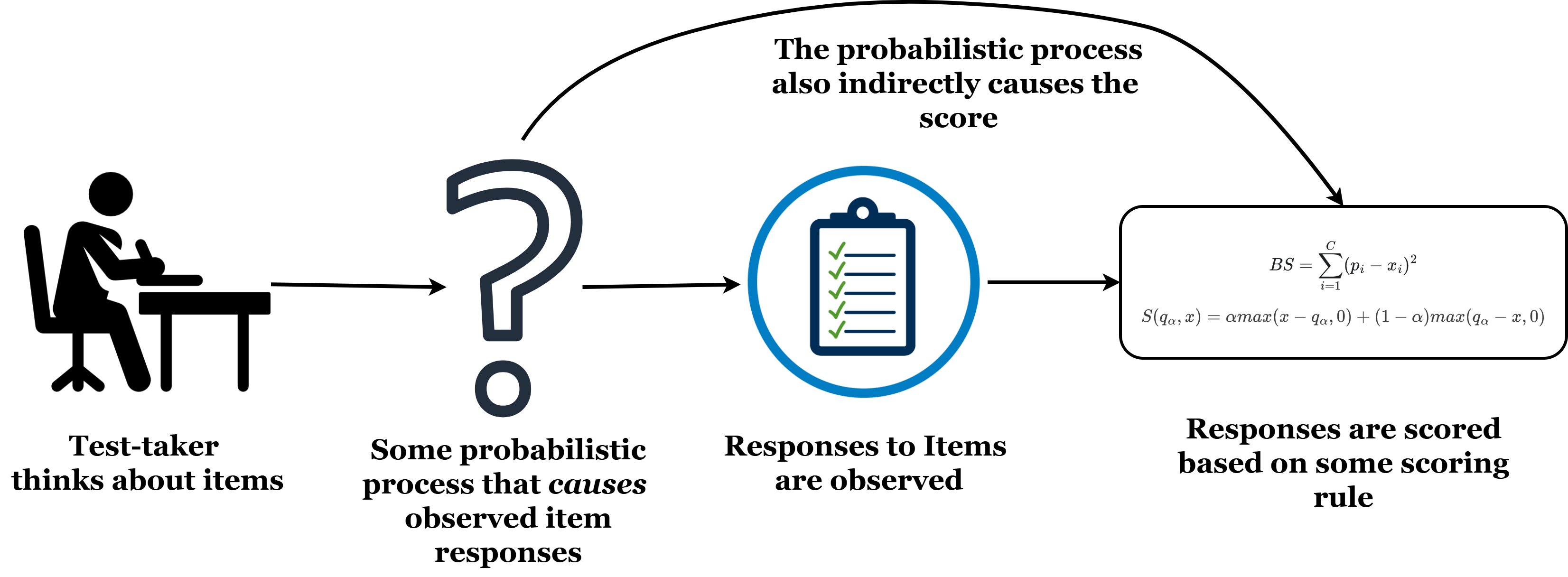
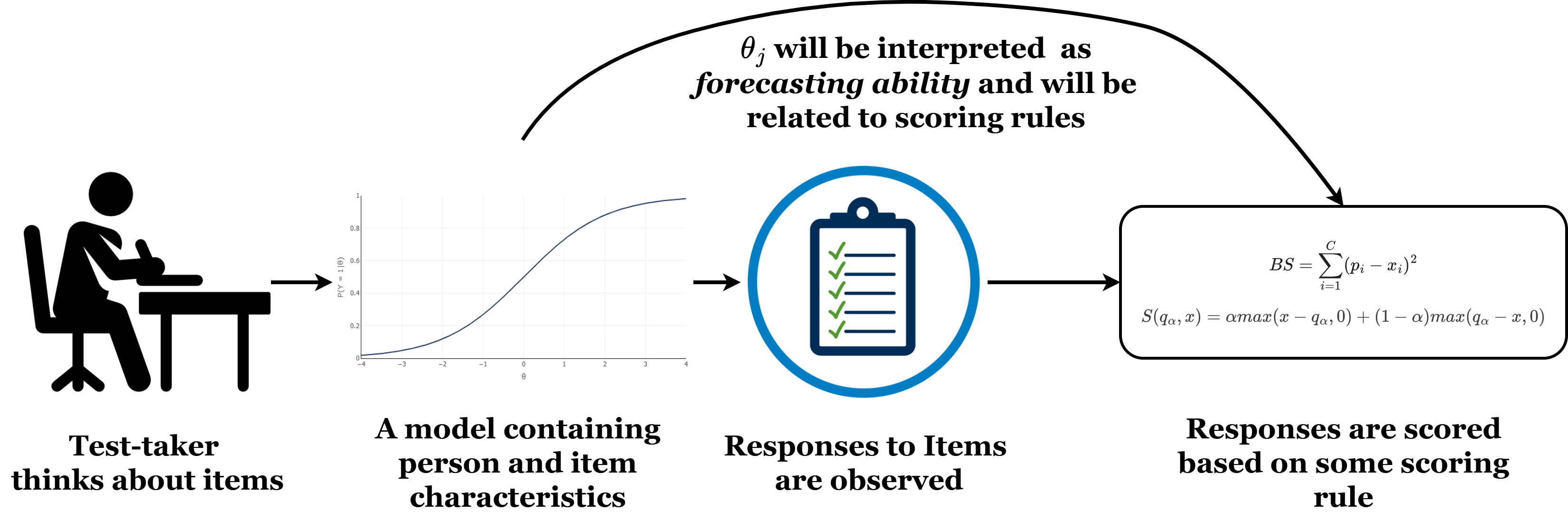
The interest of psychometrics is uncovering the probabilistic process that causes item responses.
in general, psychometric models are statistical models that predict item responses. All psychometric models include:
- Parameters defining item properties
- Parameters defining person properties
- Allow for some randomness in item responses (random measurement error)
Item response theory (IRT) models include all of these components.

Why Psychometrics and IRT?
With psychometric models, not only do we explain the observed responses, but we also obtain item characteristics and person characteristics.
Question: Can we do the same for quantile forecast items in the Forecasting Proficiency Test (FPT; Himmelstein et al., 2024)?
Historical Standardization
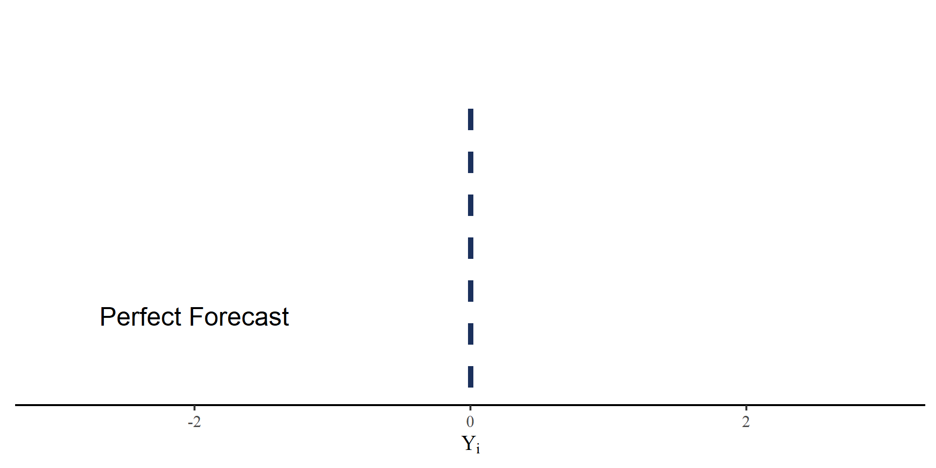
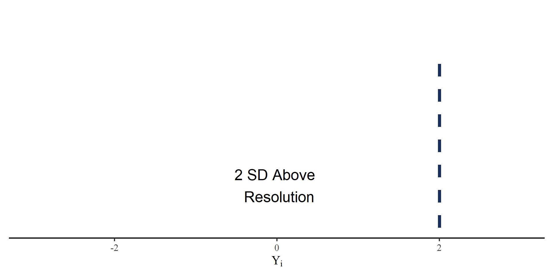
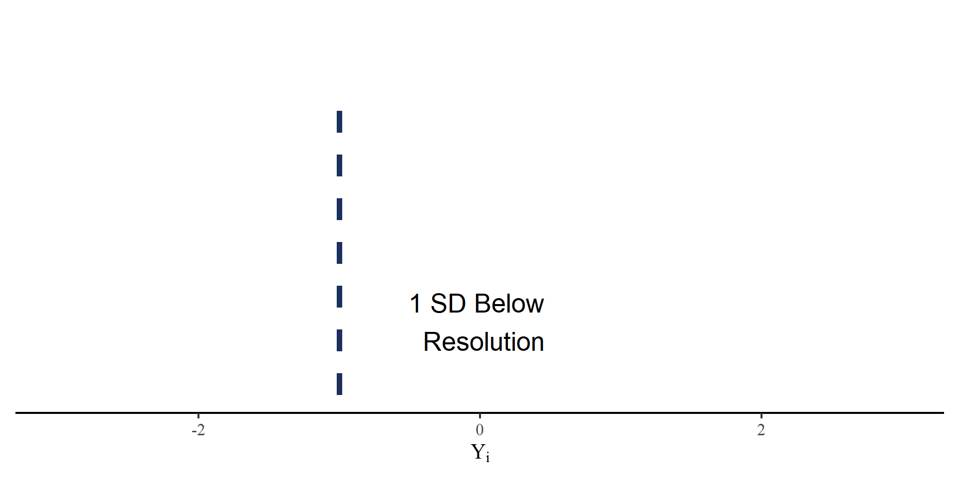
Responses to FPT quantile forecast items are on very different scales (e.g. dollars/gallon, thousands of dollars, percentages,…). We define the outcome measure, historically scaled signed error, as
\[ Y_i = \frac{\hat{Y}_i - Y_{\mathrm{res},i}}{SD_{Y_{\mathrm{hist},i}}} \]
- \(\hat{Y}_i\): Reported forecast for item \(i\) at any quantile.
- \(Y_{\mathrm{res},i}\): The resolution for item \(i\).
- \(SD_{Y_{\mathrm{hist},i}}\): The \(SD\) of the historical time series of item \(i\).
\(Y_i\): SD units away from the resolution.
Observed Distributions of Signed Error
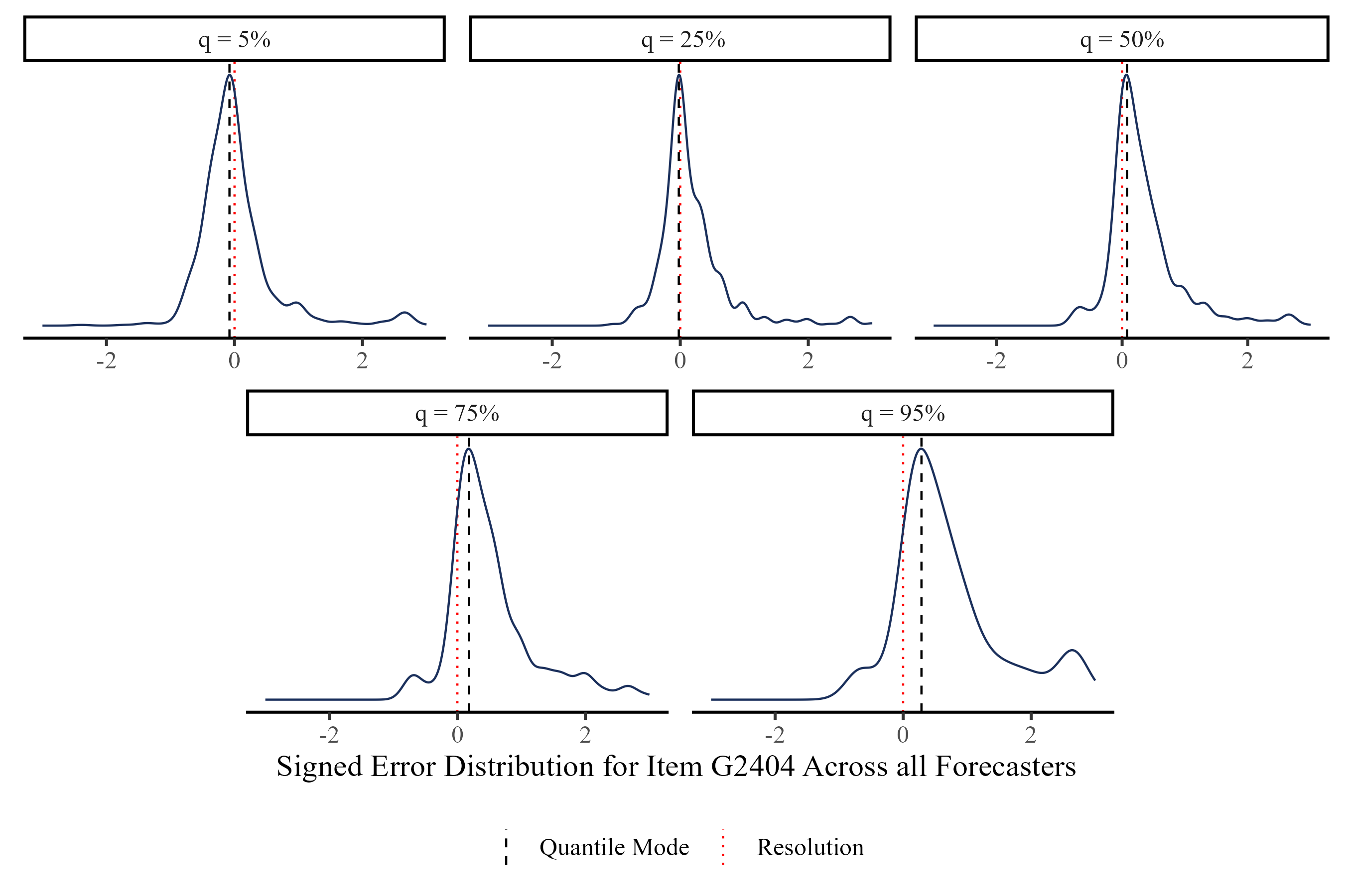

Item G2404: What will be the 12-month percentage change in the U.S. Consumer Price Index (CPI) for “Food” in the month between May 1, 2024 and May 31, 2024?
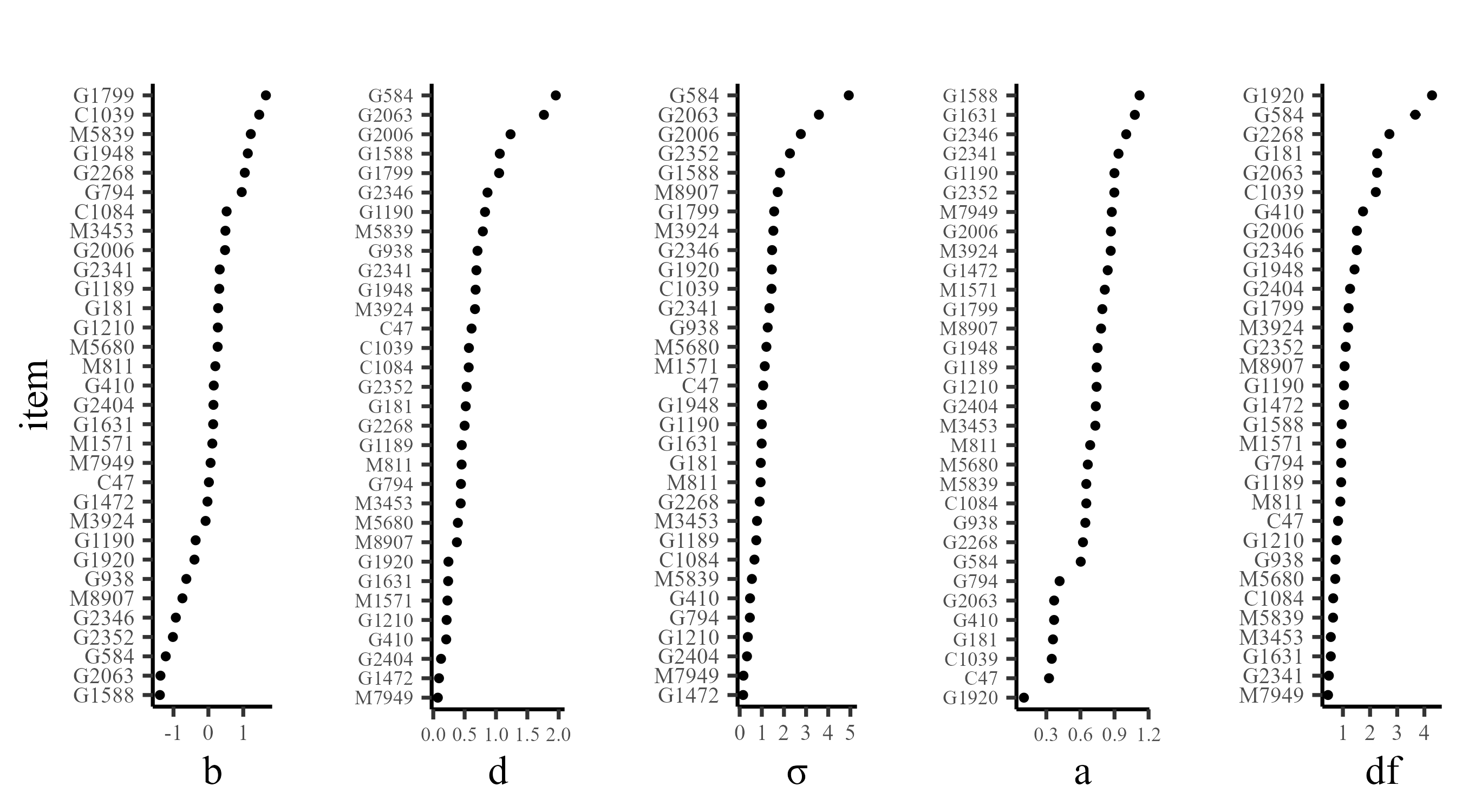
Model Estimation and Item Parameters
All models were estimated in PyMC (Abril-Pla et al., 2023) using Markov Chain Monte Carlo (MCMC) estimation (warmup = 1000, draws = 5000, ~ 40 minutes). All Rhats \(\leq 1.01\).
Person Parameter: \(\theta\)
Distribution of \(\theta\) for the 1194 forecasters (better forecasters have higher \(\theta\) values).
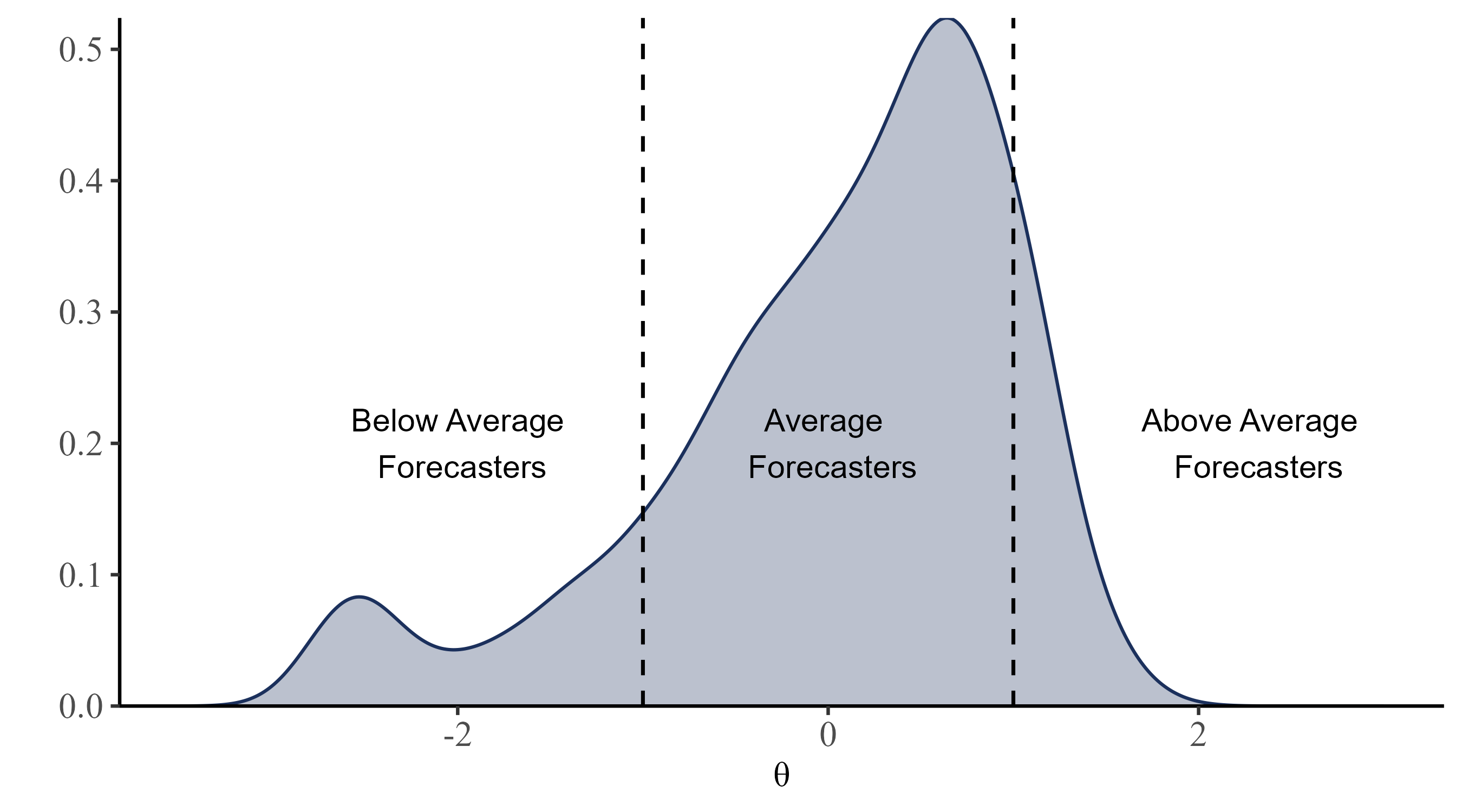
note. The scale \(\theta\) parameter was identified by enforcing a standard normal prior.
Who gets Higher \(\theta s\)?
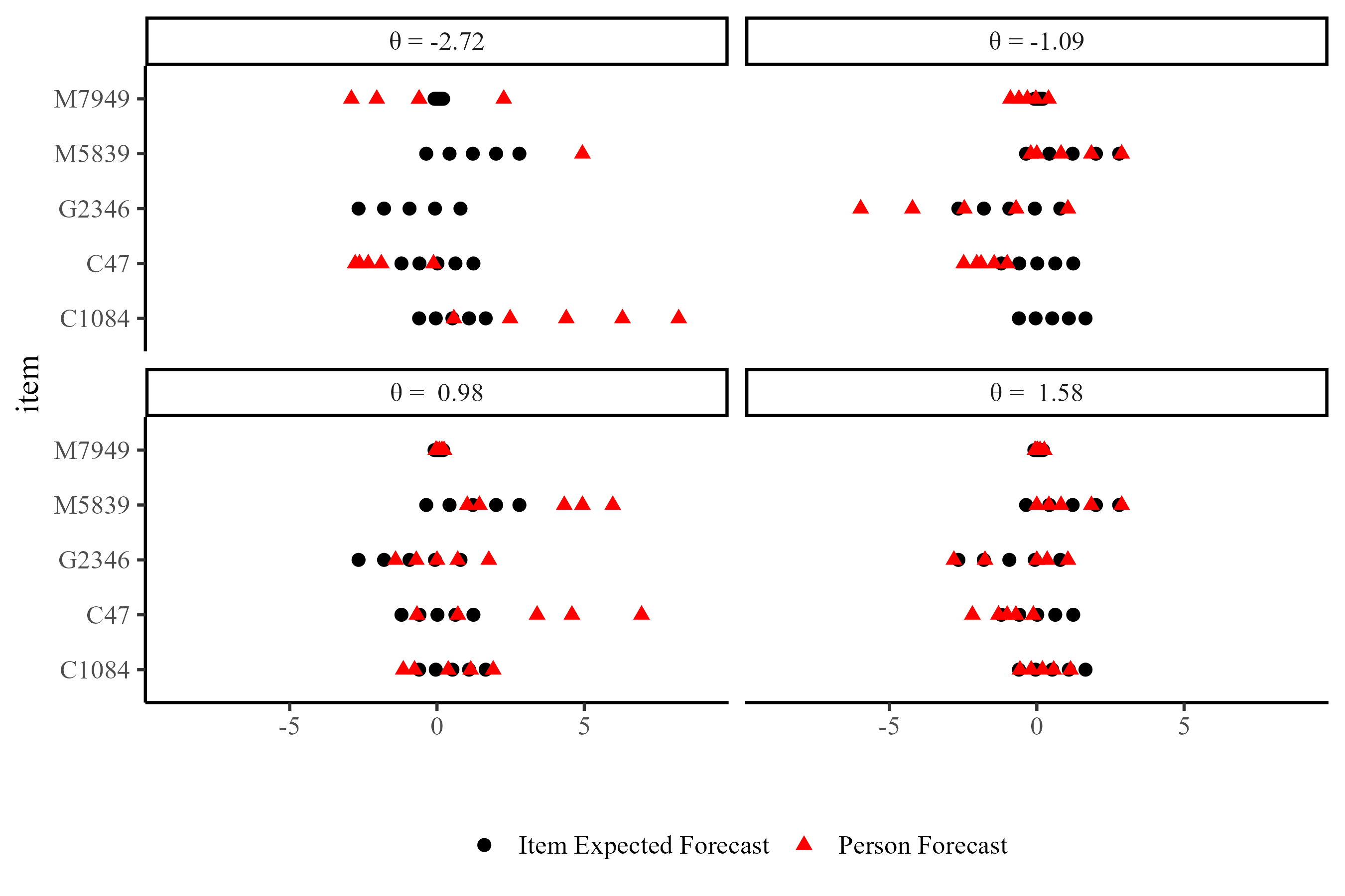
note. In the case of the two top panels, missing person forecast were outside the \(Y_{jiq} = [-9; 9]\) range.
For any set of quantile forecasts, \(\theta\) is maximized if and only if all person forecasts equal exactly the corresponding item expected forecasts.
Uncertainty Around \(\theta\) and S-Scores
\(\theta\) has less uncertainty around its estimates:
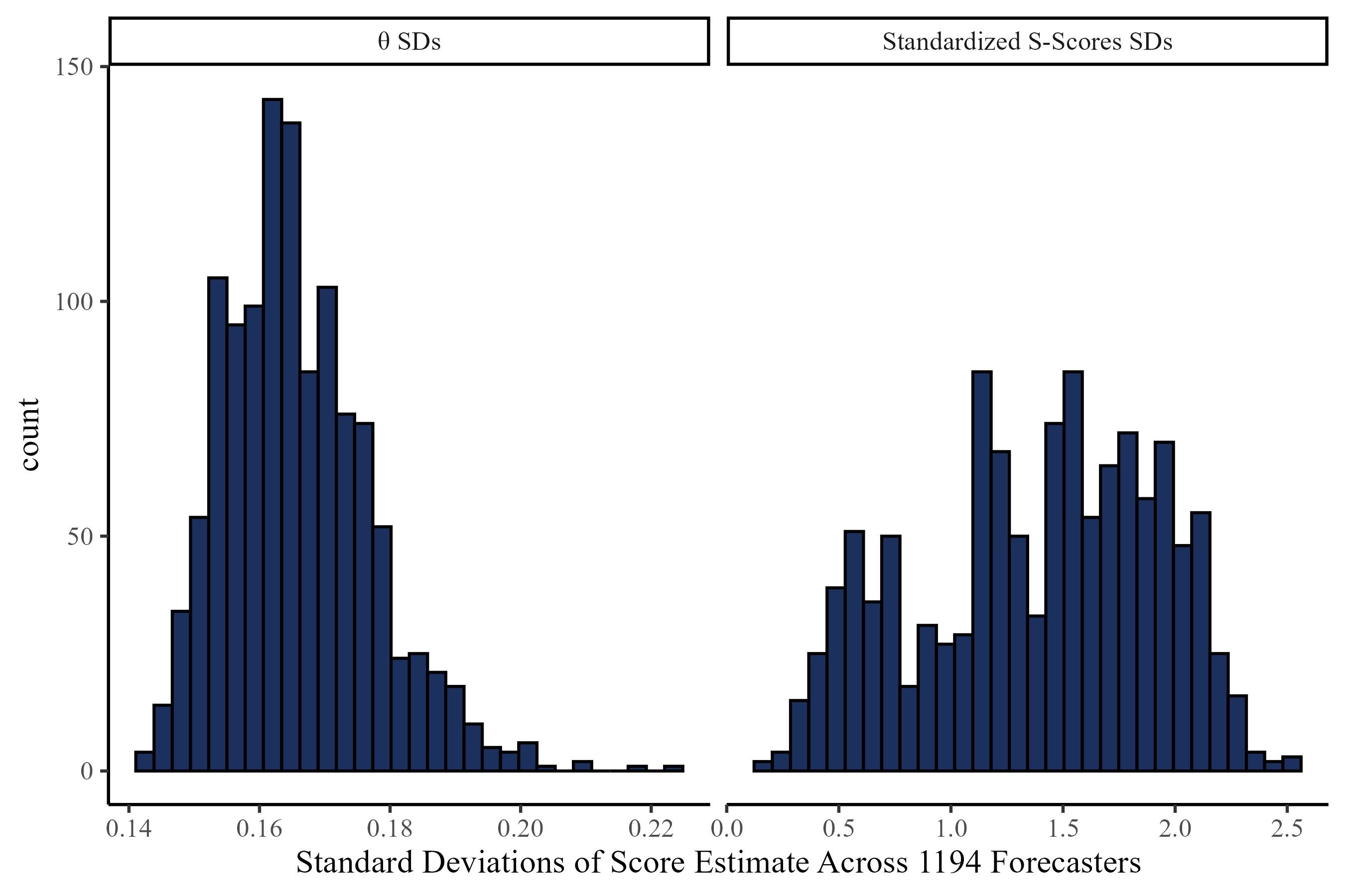
Different X-axis scale across panels
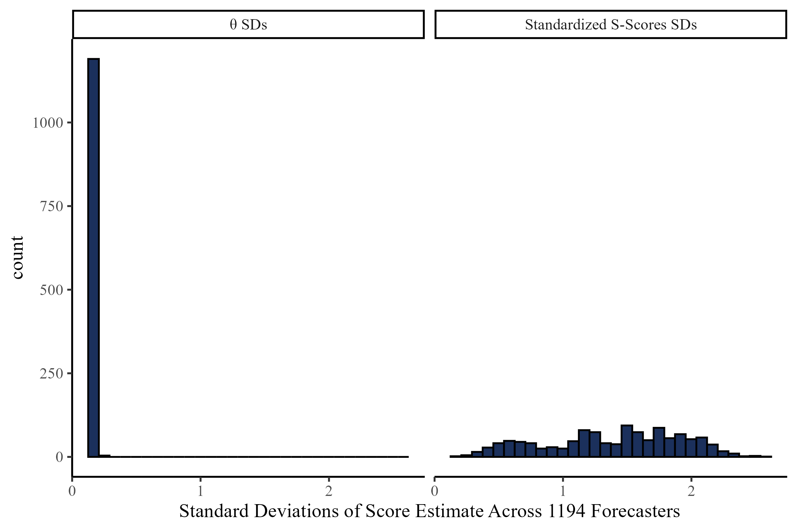
Same X-axis scale across panels
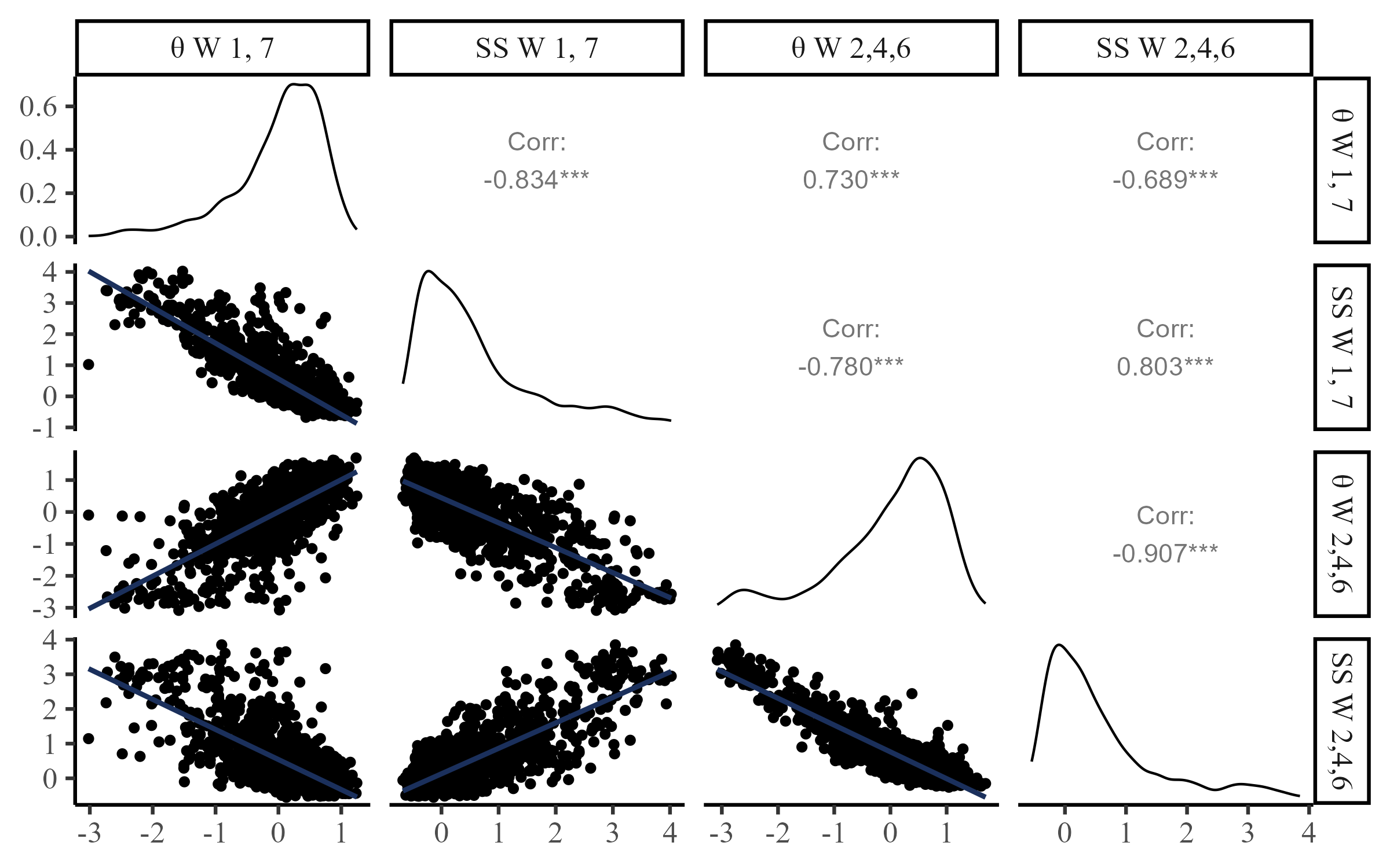
Predicting Out of Sample Accuracy
As per the study pre-registration, Waves 1 and 7 responses were treated as outcome and Waves 2,4, 6 were treated as predictors.
* SS stands for S-Score
Takeaways
- This approach captures meaningful difference across FPT items (i.e., bias, difficulty, discrimination,…)
- The \(\theta\) metric is easily understood and presents good statistical properties
- The \(\theta\) metric predicts out of sample accuracy well
\(\theta\) And S-scores?

References And Contacts
Abril-Pla, O., Andreani, V., Carroll, C., Dong, L., Fonnesbeck, C. J., Kochurov, M., Kumar, R., Lao, J., Luhmann, C. C., Martin, O. A., Osthege, M., Vieira, R., Wiecki, T., & Zinkov, R. (2023). PyMC: A modern, and comprehensive probabilistic programming framework in Python. PeerJ Computer Science, 9, e1516. https://doi.org/10.7717/peerj-cs.1516
Himmelstein, M., Zhu, S. M., Petrov, N., Karger, E., Helmer, J., Livnat, S., Bennett, A., Hedley, P., & Tetlock, P. (2024, November 18). The Forecasting Proficiency Test: A General Use Assessment of Forecasting Ability. https://doi.org/10.31234/osf.io/a7kdx
Contact: fsetti@fordham.edu

Slides and More

Stability of Parameters
Given the complexity of the FPT items, item parameters are likely to change depending on many factors. Still, there seems to be reasonable stability even after a month between Wave 1 and Wave 7 (test-retest):
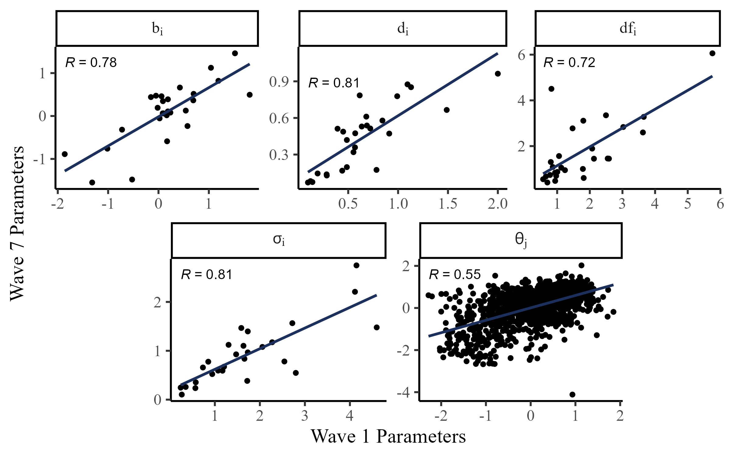
note. Only items from Waves 1 and 7. The \(a_i\) parameter requires higher sample sizes to stably estimate, so it was fixed to 1.