Measuring Forecasting Proficiency: An Item Response Theory Approach

¹Fabio Setti, ¹Leah Feuerstahler, ^2,6Sophie Ma Zhu, ^3,6Nikolay Petrov, ^4,6Ezra Karger, ^5,6Mark Himmelstein

¹Fordham University, ²University of British Columbia, ³University of Cambridge, ⁴Federal Reserve Bank of Chicago, ⁵Georgia Institute of Technology, ⁶Forecasting Research Institute

Quantile Forecasts

The Forecasting Proficiency Test (FPT; Himmelstein et al., 2024) is a test developed to measure forecasting proficiency. The FPT uses quantile forecast items:

FPT sample item:

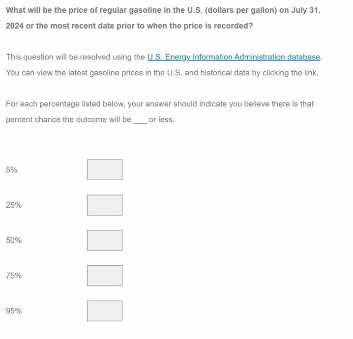
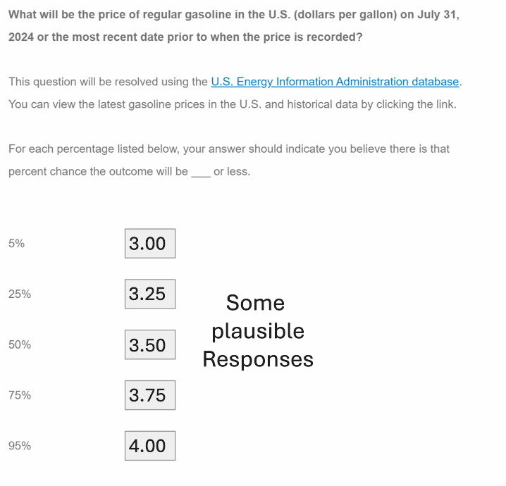
Quantile forecast items are designed to elicit an individual’s subjective cumulative distribution function (CDF) regarding a future continuous outcome

• Each individual provides 5 monotonically increasing responses

• Responses are unbounded

• Forecast accuracy is the measure of interest

GOAL: in IRT fashion, modeling forecast accuracy by positing a statistical model that accounts for both person and item features

Defining Forecast Accuracy

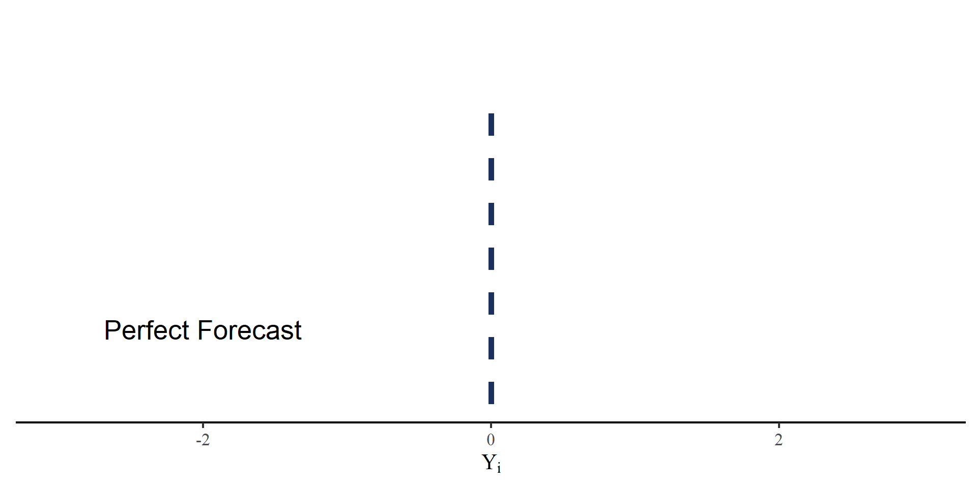
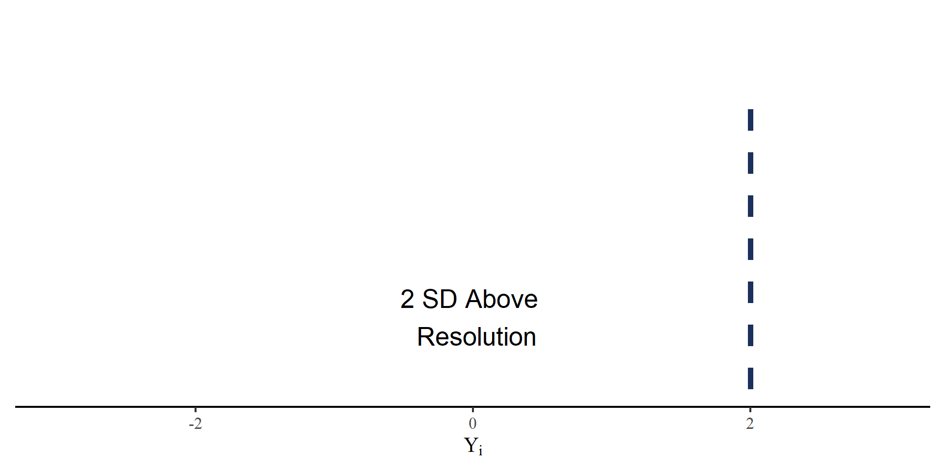
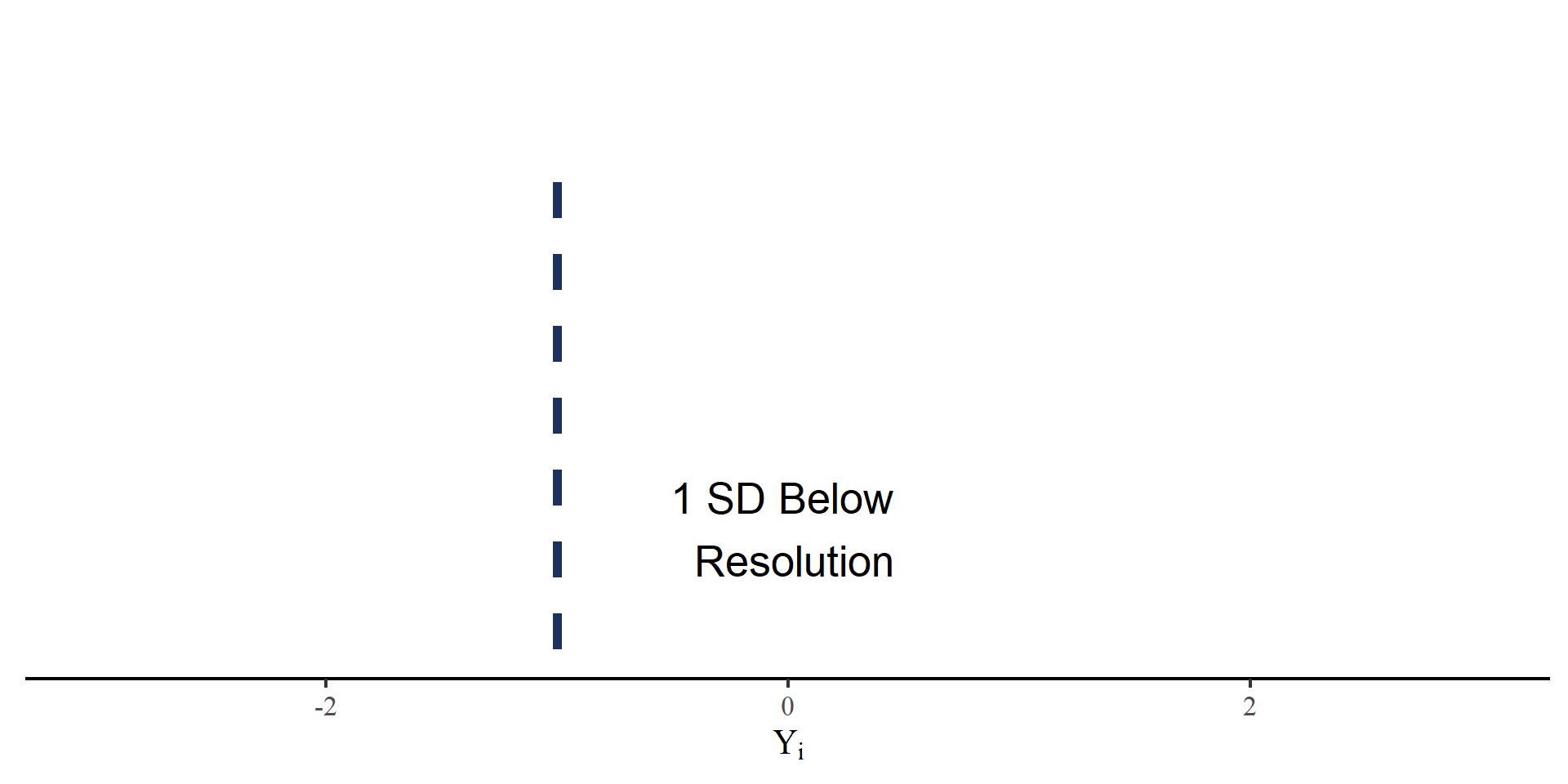
Responses to FPT quantile forecast items are on very different scale (e.g. dollars/gallon, thousands of dollars, percentages,…). We define the outcome measure, historically scaled accuracy, as

\[ Y_i = \frac{\hat{Y}_i - Y_{\mathrm{res},i}}{SD_{Y_{\mathrm{hist},i}}} \]

• \(\hat{Y}_i\): Reported forecast for item \(i\) at any quantile.
• \(Y_{\mathrm{res},i}\): The resolution for item \(i\).
• \(SD_{Y_{\mathrm{hist},i}}\): The \(SD\) of the historical time series of item \(i\).

\(Y_i\): SD units away from the resolution.

The Proposed Model

We model \(Y_{jiq}\), the accuracy of person \(j\) to item \(i\) at quantile \(q\).

\[Y_{jiq} \sim \mathrm{Student\ T}(\mu_{iq}, \sigma_{ji}, \mathrm{df}_i) \\ \mu_{iq} = b_i + Q_q \times d_i \\ \sigma_{ji} = \frac{\sigma_i}{\mathrm{Exp}[a_i \times \theta_j]}\]

\(b_i\): item bias (irreducible uncertainty)
\(d_i\): expected quantile distance. \(Q_q\) is a vector of constants that ensures monotonicity of \(\mu_{iq}\)
\(\sigma_i\): item difficulty
\(\theta_j\): Forecasting ability, the only person parameter in the model
\(a_i\): item discrimination (i.e. the magnitude of the effect of \(\theta_j\) on \(\sigma_i\))

Data Collection

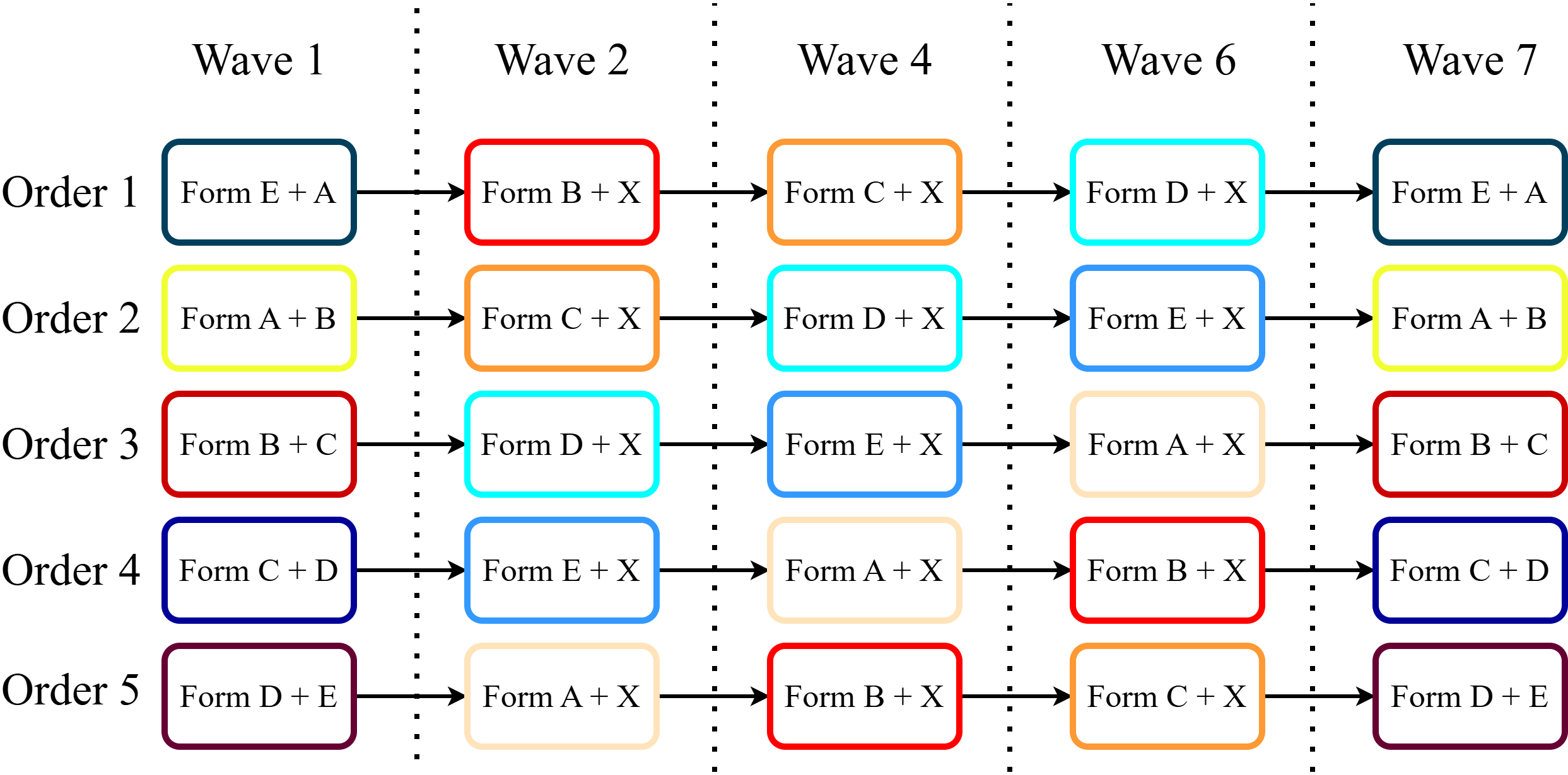
Item forecasts were collected across 5 waves of a 7 Wave study.

• 32 items divided across 6 forms (A, B, C, D, E, X) and 1194 participants
Diverse item domains: Financial, political, technology, energy…
1 week interval between waves, and 1 month from resolution at wave 7

note. The full experimental designed is detailed in both Zhu et al. (2024) and Himmelstein et al. (2024).

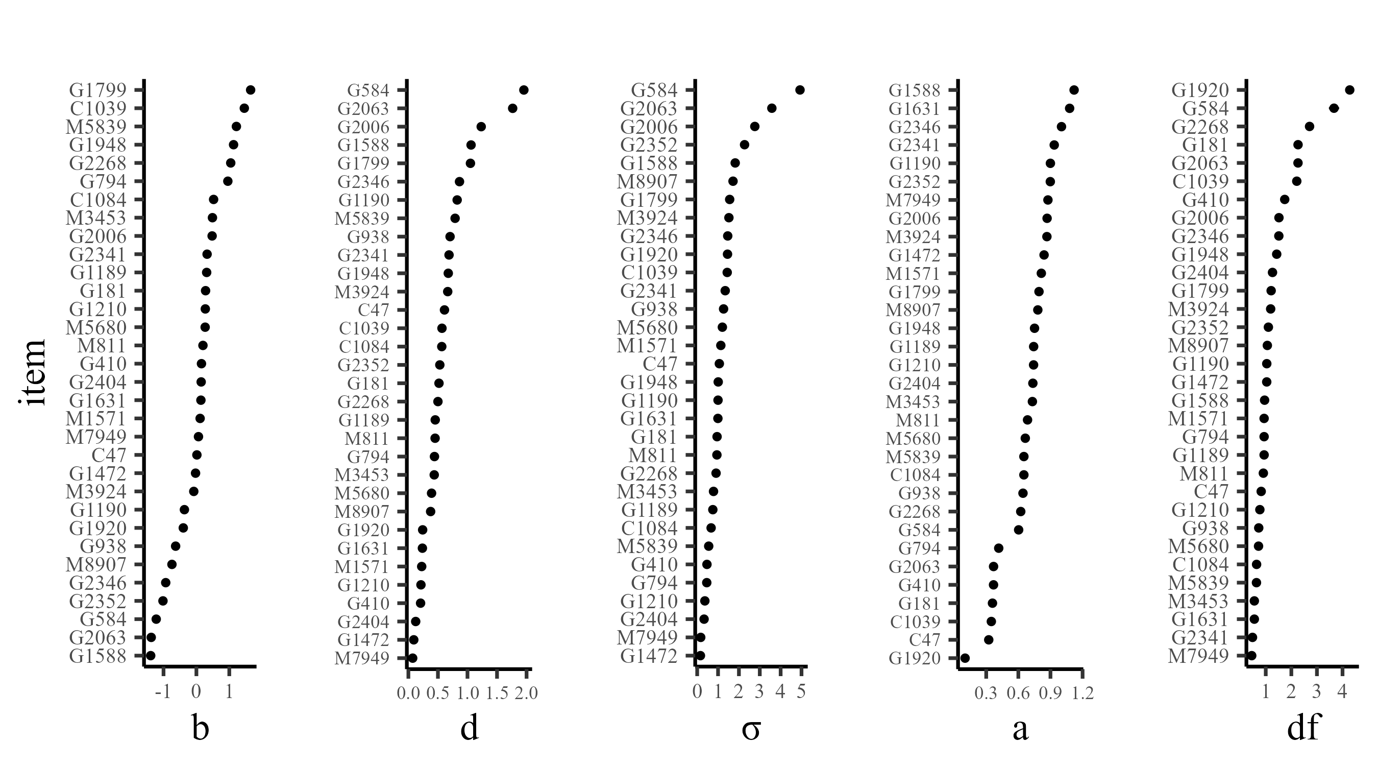
Model Estimation and Item Parameters

All models were estimated in PyMC (Abril-Pla et al., 2023) using Markov Chain Monte Carlo (MCMC) estimation (warmup = 1000, draws = 5000, ~ 40 minutes). All Rhats \(\leq 1.01\).

Person Parameter: \(\theta\)

Distribution of \(\theta\) for the 1194 forecasters (better forecasters have higher \(\theta\) values).

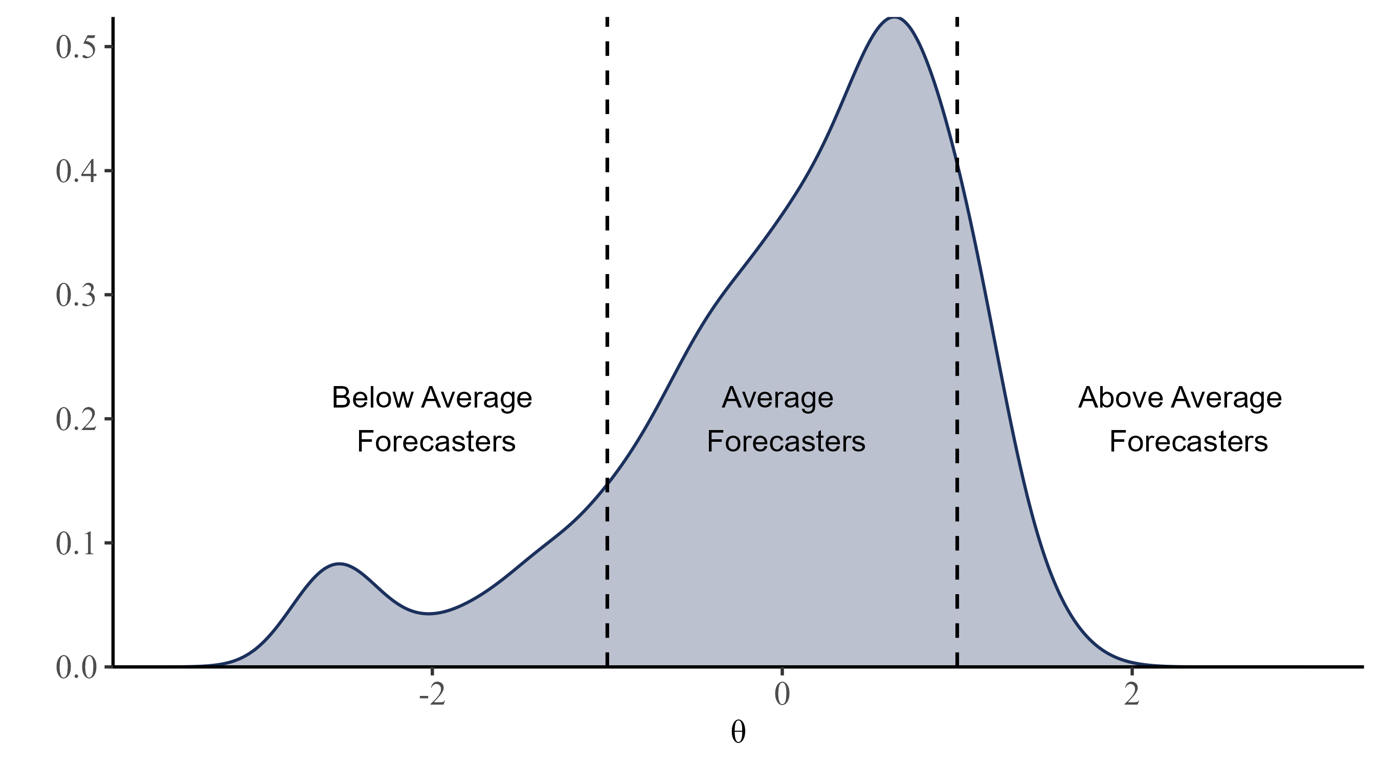
note. The scale \(\theta\) parameter was identified by enforcing a standard normal prior.

Who gets Higher \(\theta s\)?

Forecasters who consistently approach the expected forecasts are rewarded

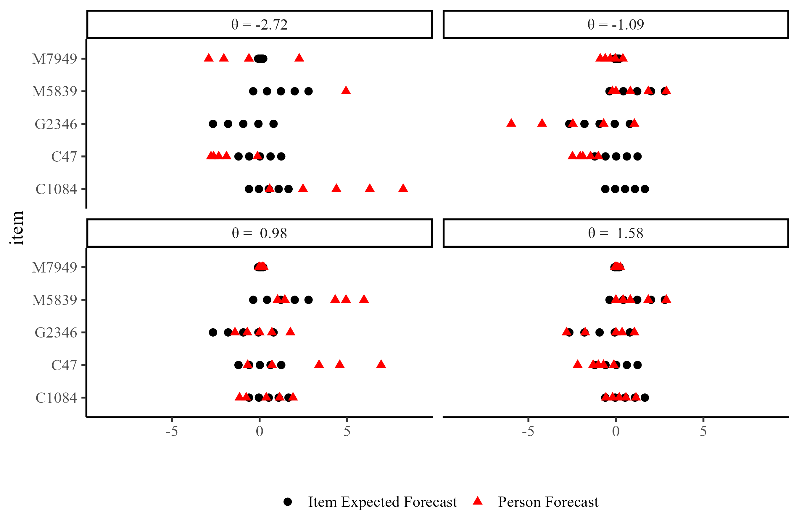
note. In the case of the two top panels, missing person forecast were outside the \(Y_{jiq} = [-9; 9]\) range.

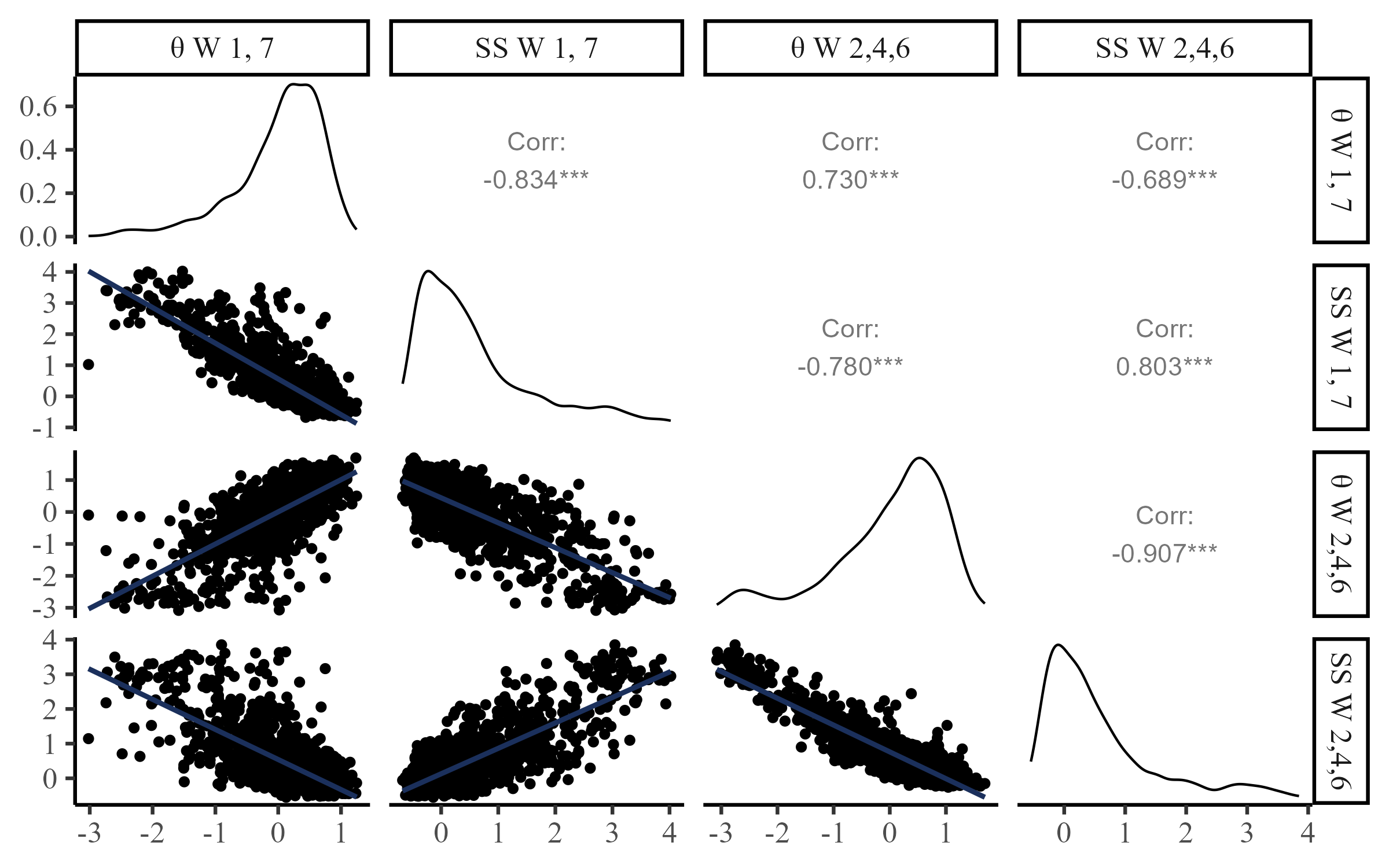
Predicting Out of Sample Accuracy

As per the study design, Waves 1 and 7 responses were treated as outcome and Waves 2,4, 6 were treated as predictors.

S-scores (SS): A proper scoring rule that is normally used to score quantile forecasts (smaller SS, better forecast)

Expected Item Information

One advantage of the \(\theta\) metric is that it allows for the calculation of expected item information, \(\mathrm{EI}(\theta)\) :

\[Y_{jiq} \sim \mathrm{Student\ T}(\mu_{iq}, \sigma_{ji}, \mathrm{df}_i) \\ \mu_{iq} = b_i + Q_q \times d_i \\ \sigma_{ji} = \frac{\sigma_i}{\mathrm{Exp}[a_i \times \theta_j]}\]

Items with higher \(\sigma_i\) measure more skilled forecasters better.
Higher \(a_i\) implies better measurement within a narrower interval of \(\theta\).
\(df_i\) functions in a similar way to \(\sigma_i\).
The parameters within \(\mu_{iq}\) do not influence \(\mathrm{E} \mathrm{I}(\theta)\) much.

note: \(\mathrm{E} \mathrm{I}(\theta)\) is computed by integrating over \(Y_{jiq}[-10;10]\).

Stability of Parameters

Given the complexity of the FPT items, item parameters are likely to change depending on many factors. Still, there seems to be reasonable stability even after a month between Wave 1 and Wave 7 (test-retest):

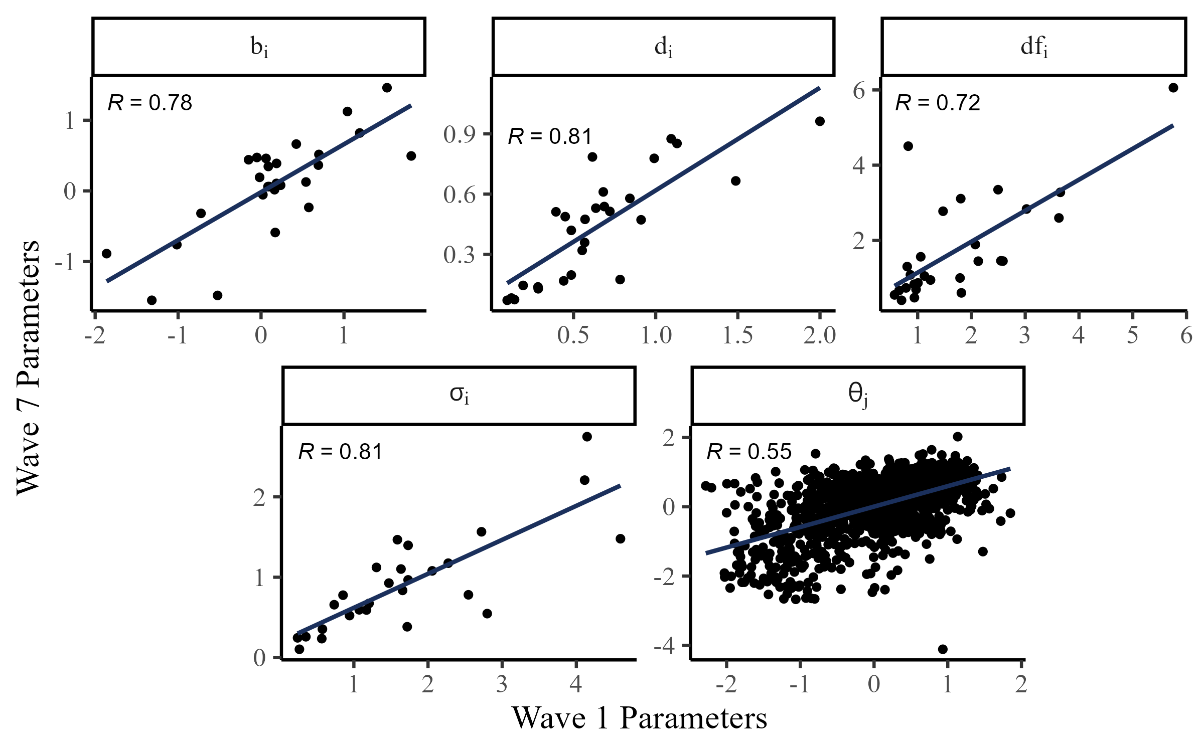
note. Only items from Waves 1 and 7. The \(a_i\) parameter requires higher sample sizes to stably estimate, so it was fixed to 1.

Takeaways

• The current approach captures meaingful difference across FPT items (i.e., bias, difficulty, discrimination,…)

• The \(\theta\) metric is easily undesrtood and viable for scoring individuals

• Item information can be calculated, although the practical uses are not as straightforward as conventional testing scenarios

Acknowledgments

Leah Feuerstahler

Mark Himmelstein

Sophie Ma Zhu

Nikolay Petrov

Ezra Karger

References And Contacts

Abril-Pla, O., Andreani, V., Carroll, C., Dong, L., Fonnesbeck, C. J., Kochurov, M., Kumar, R., Lao, J., Luhmann, C. C., Martin, O. A., Osthege, M., Vieira, R., Wiecki, T., & Zinkov, R. (2023). PyMC: A modern, and comprehensive probabilistic programming framework in Python. PeerJ Computer Science, 9, e1516. https://doi.org/10.7717/peerj-cs.1516

Himmelstein, M., Zhu, S. M., Petrov, N., Karger, E., Helmer, J., Livnat, S., Bennett, A., Hedley, P., & Tetlock, P. (2024, November 18). The Forecasting Proficiency Test: A General Use Assessment of Forecasting Ability. https://doi.org/10.31234/osf.io/a7kdx

Zhu, S. M., Budescu, D., Petrov, N., Karger, E., & Himmelstein, M. (2024, November 19). The Psychometric Properties of Probability and Quantile Forecasts. https://doi.org/10.31234/osf.io/2m4ya

Contact: fsetti@fordham.edu

Slides Link

Appendix

Negative Log-Likelihood of \(\theta\)

Negative log-likelihood function of \(\theta\) given item parameters and participant response:

Between Item Parameters Correlation

Between Item Parameters Correlations

	a	b	d	df	sigma
a	1.00	-0.17	0.00	-0.57	-0.04
b	-0.17	1.00	-0.33	-0.18	-0.51
d	0.00	-0.33	1.00	0.35	0.86
df	-0.57	-0.18	0.35	1.00	0.52
sigma	-0.04	-0.51	0.86	0.52	1.00