library(Seurat)
library(dplyr)
library(data.table)
library(stringr)
library(Gviz)
library(ggplot2)
library(ggthemes)
library(rtracklayer)

#load gene based analysis Seurat object
dge.obj = readRDS("./neuro_DGE.RDS")Downstream analysis on scRNA-seq from human neuronal differentiation using SCALPEL
Note
Note: Install scalpelR for downstream analysis
For execution of several function used in this downstream analysis with SCALPEL, we will implemented the R package scalpelR that can be installed from its Github page as:
install.packages("devtools")
devtools::install_github("Franzx7/scalpelR")

library(scalpelR)
1 Introduction
In this exemple, we did a gene and isoform based single-cell analysis from this Drop-seq single-cell dataset. Using Seurat, we first performed a standard single-cell gene-level analysis of the human neuronal differentiation dataset, which enabled the identification of distinct cell populations.
#Visualize gene based sc cells
DimPlot(dge.obj, label=T, repel = T, pt.size = 1., label.size = 6) %>% theme_umap() +
    ggtitle("iPS & NPC cells clusters")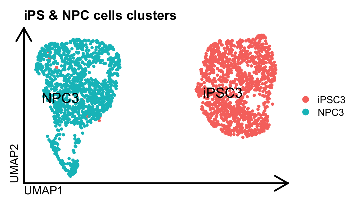
Prior to obtain this final clusters of population, we performed some quality filtering steps to obtain this set of reliable cells. Using those same cells barcode tags, we executed SCALPEL on this Drop-seq based single-cell dataset. All the information required to run SCALPEL can be found on its Github page.
Note
Note: SCALPEL requires the FASTQ, BAM and Gene count expression associated to each sample for its execution. For Drop-seq experiments, the BAM and Gene count expression can be obtained using the Drop-seq tools and for 10x Genomics experiments, the BAM and Gene count expression can be obtained using the CellRanger pipeline.
SCALPEL execution can be performed on a specific cell population using the - -barcodes argument option.
Following SCALPEL execution, a result folder is generated that contains all the information required to perform downstream analysis.
> tree -L 1 scalpel_output
scalpel_output
├── DIU_table.csv
├── hiPSCs_APADGE.txt
├── hiPSCs_filtered.bam
├── hiPSCs_filtered.bam.bai
├── hiPSCs_seurat.RDS
├── iDGE_seurat.RDS
├── NPCs_APADGE.txt
├── NPCs_filtered.bam
├── NPCs_filtered.bam.bai
├── NPCs_seurat.RDS
└── Runfiles

2 directories, 10 files
2 Downstream analysis of SCALPEL results
2.1 Loading isoform based Seurat object
Let’s load the isoform-based Seurat object generated by SCALPEL using the reliable cell barcodes obtained from the gene-based analysis:
idge.obj = readRDS("./iDGE_seurat.RDS")
idge.obj
An object of class Seurat
68874 features across 2535 samples within 1 assay
Active assay: RNA (68874 features, 3837 variable features)
3 layers present: data, counts, scale.data
2 dimensional reductions calculated: pca, umap2.2 Quality filtering on low expressed isoforms features
For this analysis, we already used a reliable set of cells obtained from the gene-based analysis. However, we can still perform some filtering steps to discard lowly expressed isoforms features that are not informative. For example, we can filter out isoforms that are detected in less than 3 cells:
# Filter out isoforms that are detected in less than 3 cells
idge.obj = subset(idge.obj, features = rownames(idge.obj)[Matrix::rowSums(idge.obj@assays$RNA@counts > 0) >= 3])
2.3 Dimensionality reduction and clustering
Let’s perform the dimensionality reduction and clustering on this isoform-based Seurat object:
# Standard workflow for dimensionality reduction and clustering (Adjust the parameters)
idge.obj = NormalizeData(idge.obj)
# as isoform data is more sparse and noisy, we recommend to use a higher number of variable features
idge.obj = FindVariableFeatures(idge.obj, nfeatures = 4000)
idge.obj = ScaleData(idge.obj)
idge.obj = RunPCA(idge.obj, npcs = 50)
idge.obj = RunUMAP(idge.obj, dims = 1:30)

#Clustering
idge.obj = FindNeighbors(idge.obj, dims = 1:30)
idge.obj = FindClusters(idge.obj, resolution = 0.5)
idge.obj$Clusters = idge.obj$seurat_clusters
Now, we can visualize the clusters obtained from this isoform-based analysis. We can observe that while briging a new layer of information, the isoform quantification conserves the cell type specificity identified from the gene-based analysis
# Filter out isoforms that are detected in less than 3 cells
DimPlot(idge.obj, group.by="Clusters", label=T, repel = T, pt.size = 1., label.size = 6) %>% theme_umap() + ggtitle("iPS & NPC cells clusters (isoform-based)")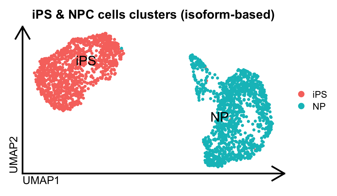
2.4 Differential isoform expression analysis
We can perform a differential isoform expression analysis between the different clusters obtained from the isoform-based analysis. For example, let’s perform a differential isoform expression analysis between the iPSC and NP cell populations:
diu.table = scalpelR::FindIsoforms(
    seurat_obj = idge.obj,
    group_by = "Clusters",
    assay="RNA",
    threshold_pval = 0.05)

print(diu.table)
Aggregating counts in conditions… Performing filtering and comparison test… |++++++++++++++++++++++++++++++++++++++++++++++++++| 100% elapsed=51s
                  gene_tr gene_name transcript_name   iPS    NP      p_value
                   <char>    <char>          <char> <num> <num>        <num>
   1:   ABCE1***ABCE1-201     ABCE1       ABCE1-201   355    93 0.0004997501
   2:   ABCE1***ABCE1-202     ABCE1       ABCE1-202    97    90 0.0004997501
   3:   ABCE1***ABCE1-203     ABCE1       ABCE1-203   267    88 0.0004997501
   4:     ABI2***ABI2-201      ABI2        ABI2-201   154   209 0.0004997501
   5:     ABI2***ABI2-208      ABI2        ABI2-208   232   104 0.0004997501
  ---
3069: SCARB2***SCARB2-225    SCARB2      SCARB2-225    54    44 0.0094952524
3070: ZNF429***ZNF429-201    ZNF429      ZNF429-201    24     9 0.0094952524
3071: ZNF429***ZNF429-202    ZNF429      ZNF429-202    14     9 0.0094952524
3072: ZNF429***ZNF429-205    ZNF429      ZNF429-205     5    14 0.0094952524
3073: ZNF429***ZNF429-208    ZNF429      ZNF429-208     5     5 0.0094952524
      statistic p_value_adjusted
          <num>            <num>
   1: 51.570918      0.004359955
   2: 51.570918      0.004359955
   3: 51.570918      0.004359955
   4: 50.017008      0.004359955
   5: 50.017008      0.004359955
  ---
3069:  9.907011      0.048981042
3070: 10.927779      0.048981042
3071: 10.927779      0.048981042
3072: 10.927779      0.048981042
3073: 10.927779      0.048981042
We can visualize a particular gene expression, for example the gene EIF1, that have differentially expressed isoforms between the iPSC and NPC populations:
gene.tab = diu.table %>% dplyr::filter(gene_name == "EIF1")
print(gene.tab)
gene_tr gene_name transcript_name iPS NP p_value statistic
<char> <char> <char> <num> <num> <num> <num>
1: EIF1***EIF1-201 EIF1 EIF1-201 2517 1938 0.0004997501 386.0618
2: EIF1***EIF1-204 EIF1 EIF1-204 5169 1799 0.0004997501 386.0618
p_value_adjusted
<num>
1: 0.004359955
2: 0.0043599552.5 Visualization of isoform expression in cells
2.5.1 UMAP
We can visualize the expression of these differentially expressed isoforms in the cells using a UMAP plot using Seurat. For example, let’s visualize the expression of the two differentially expressed isoforms of the gene EIF1:
Seurat::FeaturePlot(idge.obj,
    features = gene.tab$gene_tr,
    pt.size = 1,
    label.size=6,
    order=T,
    label=T,
    cols = c("gray80", "red"))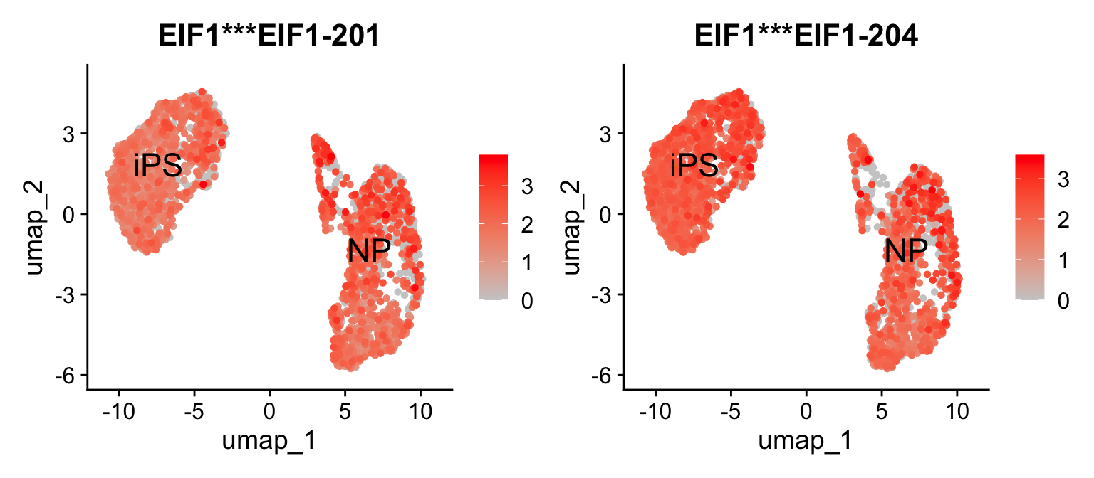
2.5.2 Violin plots
Aditionally, we can visualize the expression of these differentially expressed isoforms within the condition using violin plot as:
p1 = scalpelR::plotExpression(
    seurat_obj = idge.obj,
    features = gene.tab$gene_tr,
    group_var = "Clusters",
    plot = "group")

p2 = scalpelR::plotExpression(
    seurat_obj = idge.obj,
    features = gene.tab$gene_tr,
    group_var = "Clusters",
    plot = "features")

list(p1, p2) %>% patchwork::wrap_plots(ncol=1)
Using features as id variables
Using features as id variables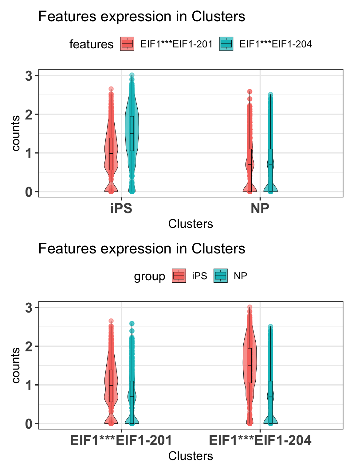
2.6 Visualization of read coverage on the genome
Furthermore, we can visualize the read coverage of these differentially expressed isoforms using the BAM files generated by SCALPEL. For example, let’s visualize the read coverage of the two differentially expressed isoforms of the gene EIF1.
As we used a curated set of cell barcodes from the gene-based analysis to run SCALPEL, the BAM files generated by SCALPEL already contains only the reads from those reliable cells. Therefore, we can directly use these filtered BAM files to visualize the read coverage of the differentially expressed isoforms. However, if you want to visualize the read coverage of a specific cell population, you can filter the BAM files using the cell barcodes associated to that population and scalpelR subsetBAM as:
ips_barcodes = dplyr::filter(idge.obj[[]], Clusters=="iPS") %>% rownames()
np_barcodes = dplyr::filter(idge.obj[[]], Clusters=="NP") %>% rownames()

# Filter BAM file to obtain reads from a specific cell population
#IPS population
scalpelR::subsetBAM(
    bam_file = "./scalpel_output/hiPSCs_filtered.bam",
    barcodes = ips_barcodes,
    output_file = "./subset_ips_filtered.bam",
    tag = "XC",
    cores = 4)

#NP population
scalpelR::subsetBAM(
    bam_file = "./scalpel_output/NPCs_filtered.bam",
    barcodes = ips_barcodes,
    output_file = "./subset_np_filtered.bam",
    tag = "XC",
    cores = 4)

#Plot coverage using the subset BAM files and GTF annotation reference
gtrack = rtracklayer::import("./gencode.v41.annotation.gtf.gz")
scalpelR::CoveragePlot(
    genome_gr = gtrack,
    bamfiles = c("IPS"="./subset_ips_filtered.bam",
                 "NP"="./subset_np_filtered.bam"),
    gene_in = "EIF1",
    genome_sp = "hg38")
$`BAM file:`
IPS NP
"~/Projects/iPS_filtered.bam" "~/Projects/NP_filtered.bam"
$`Gene:`
[1] "EIF1"
$`Transcripts:`
NULL
$`Genome annotation org:`
[1] "hg38"Building Gene Track...Building Alignment Track...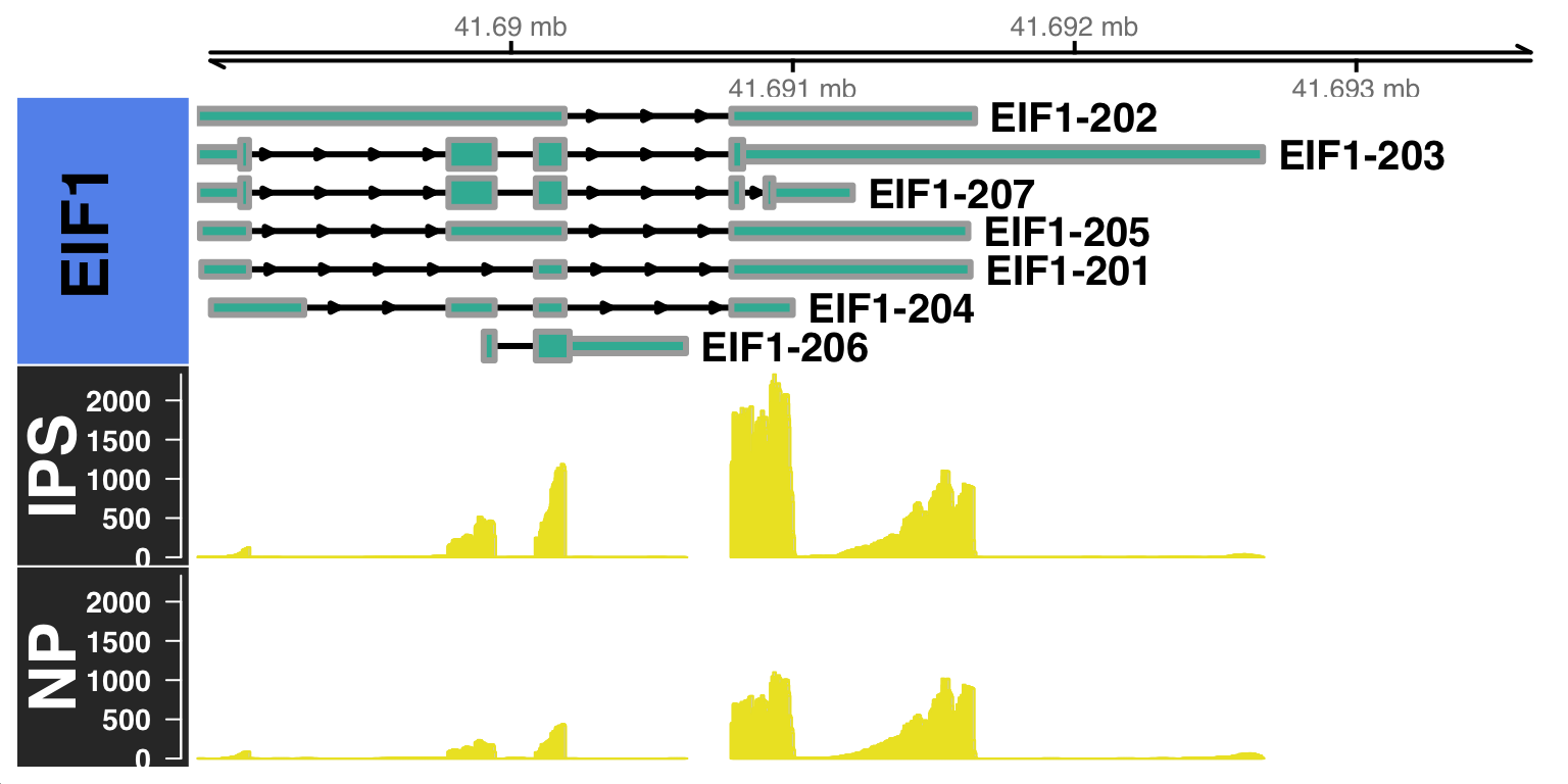
By default, the CoveragePlot function will plot all the isoforms of the gene of interest. However, you can also specify a set of isoforms to plot using the features argument option. Furthermore, you can also specify the distance to zoom from the 3’UTR using the distZOOM argument option as:
scalpelR::CoveragePlot(
    genome_gr = gtrack,
    bamfiles = c("IPS"="~/Projects/iPS_filtered.bam",
                 "NP"="~/Projects/NP_filtered.bam"),
    features = gene.tab$transcript_name,
    gene_in = "EIF1",
    genome_sp = "hg38",
    distZOOM = 2000)
$`BAM file:`
IPS NP
"~/Projects/iPS_filtered.bam" "~/Projects/NP_filtered.bam"
$`Gene:`
[1] "EIF1"
$`Transcripts:`
[1] "EIF1-201" "EIF1-204"
$`Genome annotation org:`
[1] "hg38"Building Gene Track...Building Alignment Track...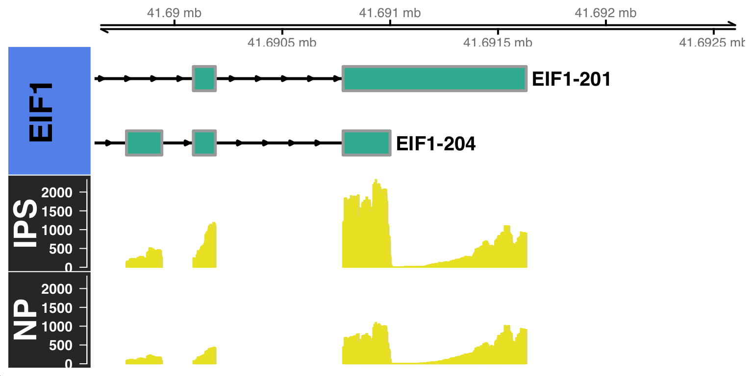
2.7 3’UTR length analysis in single-cells
Using the isoform quantification obtained from SCALPEL, and the genome annotation reference, we can estimate the 3’UTR length of each isoform in each cell. For this, we can use the function scalpelR::weightedUTR_cell as:
utr3length_tab = scalpelR::weightedUTR_cell(
    seurat_obj = idge.obj,
    annotation_gr = gtrack,
    group.by = "Clusters",
    assay = "RNA"
)
Processing annotation file...(1/3)Processing isoform expression...(2/3)Integrating Seurat metadata...(3/3)print(utr3length_tab) cells group wUTRlength.cell
<char> <char> <num>
1: AAAAAAGAACCC-1 iPS 426.7257
2: AAAAAAGAACTG-1 iPS 309.9807
3: AAAAAATGTAAC-1 iPS 284.2699
4: AAAAGAATCGGC-1 iPS 206.4187
5: AAAAGTCAACTA-1 iPS 459.1815
---
2531: TTTTCAGAGTTT-2 NP 549.5643
2532: TTTTCGCAATTC-2 NP 565.8120
2533: TTTTGGCTCAGT-2 NP 241.0014
2534: TTTTGTCACCTT-2 NP 407.8529
2535: TTTTTCCGTACG-2 NP 301.0732Then, based on this metric, we can visualize the 3’UTR length distribution in the different cell populations using plots as:
utr3length_tab %>%
    ggplot2::ggplot(aes(x=group, y=wUTRlength.cell, fill=group)) +
    geom_jitter(na.rm=T, size=.5) +
    ggplot2::geom_violin(scale="width", trim=T, na.rm = T, alpha=.6) +
    ggplot2::geom_boxplot(fill="white", width=.3) +
    ggplot2::ylim(c(0,1000)) +
    ggplot2::ggtitle("average 3'UTR length distribution per cell") +
    ggplot2::theme(title = element_text(size=9)) +
    ggplot2::theme_bw(base_size = 9)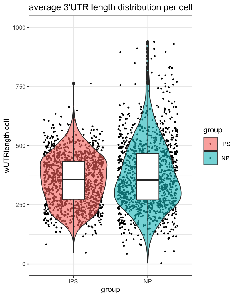
3 Further downstream analysis
Using the R Seurat Object generated by SCALPEL, you can perform further downstream analysis in the same way as a standard gene-based Seurat object. For example, you can perform trajectory analysis using Monocle3, etc…
For more information, please refer to the Seurat documentation here.