class: title-slide # Performance evaluation and hyperparameter tuning of statistical and machine-learning models using spatial data <html><div style='float:left'></div><hr color='#EB811B' size=1px width=796px></html> ### Patrick Schratz<sup>1</sup>, Jannes Muenchow<sup>1</sup>, Jakob Richter<sup>2</sup>, Alexander Brenning<sup>1</sup> <p style="margin-left:15px;"> <br> Kolloquium (Institute of Statistics), Munich, 20 Jun 2018 <br><br> <i class="fa fa-university"></i> <sup>1</sup> Department of Geography, GISciene group, University of Jena <a href="http://www.geographie.uni-jena.de/en/Geoinformatik_p_1558.html"><i class="fa fa-external-link"></i></a> <br> <i class="fa fa-university"></i> <sup>2</sup> Department of Statistics, TU Dortmund <a href="https://www.statistik.tu-dortmund.de/aktuelles.html"><i class="fa fa-external-link"></i></a> <br><br> <i class="fa fa-home"></i> <a href="https://pat-s.github.io">https://pat-s.github.io</a>   <i class="fa fa-twitter"></i> <a href="https://twitter.com/pjs_228">@pjs_228</a>   <i class="fa fa-github"></i> <a href="https://github.com/pat-s">@pat-s</a>   <i class="fa fa-stack-exchange"></i> <a href="https://stackoverflow.com/users/4185785/pat-s">@pjs_228</a>   <br> <i class="fa fa-envelope"></i> <a href="patrick.schratz@uni-jena.de">patrick.schratz@uni-jena.de</a>  <i class="fa fa-linkedin"></i> <a href="https://www.linkedin.com/in/patrick-schratz/">Patrick Schratz</a>  </p> <div class="my-header"><img src="figs/life.jpg" style="width = 5%;" /></div> --- layout: true <div class="my-header"><img src="figs/life.jpg" style="width = 5%;" /></div> --- # Outline .font150[ 1. Introduction 2. Data and study area 3. Methods 4. Results 5. Discussion ] --- class: inverse, center, middle # Introduction <html><div style='float:left'></div><hr color='#EB811B' size=1px width=720px></html> --- # Introduction ### \# Whoami - "Data Scientist" - Studied B.Sc. **Geography** & M.Sc. **Geoinformatics** at University of Jena - Self-taught programmer - Interested in model optimization, R package development, server administration #### Contributions to `mlr` - Integrated new sampling scheme for CV: Spatial sampling - Redesigned the tutorial site (`mkdocs`-> `pkgdown`) - Added getter for inner resampling indices - more to come ;) --- # Introduction .pull-left[ ### LIFE Healthy Forest <i class="fa fa-tree"></i> Early detection and advanced management systems to reduce forest decline by invasive and pathogenic agents. **Main task**: Spatial (modeling) analysis to support the early detection of various pathogens. ## Pathogens <i class="fa fa-bug"></i> * Fusarium circinatum * **Diplodia sapinea** (<i class="fa fa-arrow-right"></i> needle blight) * Armillaria root disease * Heterobasidion annosum ] .pull-right[ .center[ 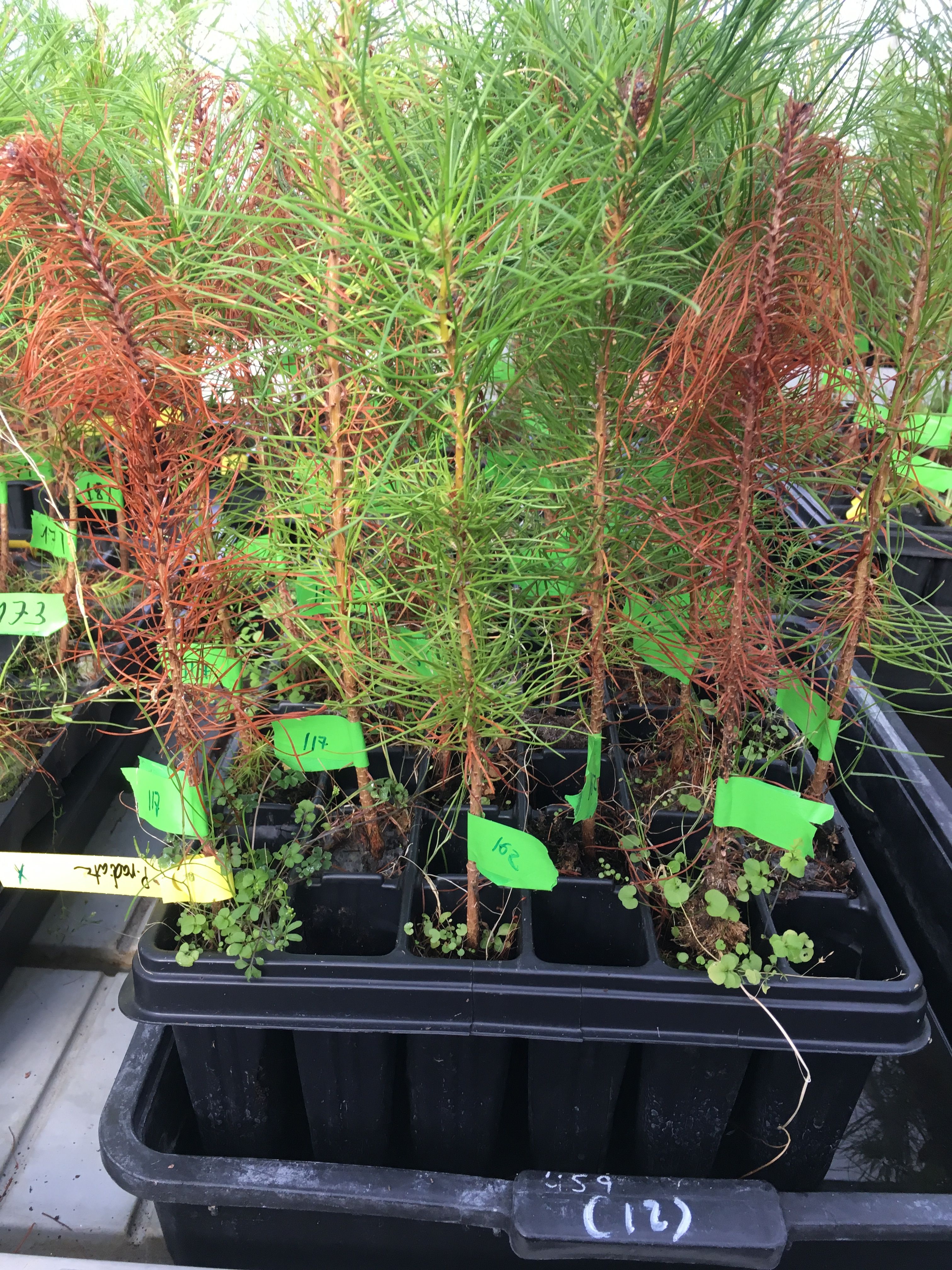 .font70[**Fig. 1:** Needle blight caused by **Diplodia pinea**] ] ] --- # Introduction ## Motivation * Find the model with the **highest predictive performance**. * Results are assumed to be representative for data sets with similar predictors and different pathogens (response). * Be aware of **spatial autocorrelation** <i class="fa fa-exclamation-triangle"></i> * Analyze differences between spatial and non-spatial hyperparameter tuning (no research here yet!). * Analyze differences in performance between algorithms and sampling schemes in CV (both performance estimation and hyperparameter tuning) --- class: inverse, center, middle # Data <i class="fa fa-database"></i> & Study Area <i class="fa fa-map"></i> <html><div style='float:left'></div><hr color='#EB811B' size=1px width=720px></html> --- # Data <i class="fa fa-database"></i> & Study Area <i class="fa fa-map"></i> .code70[ ``` ## Skim summary statistics ## n obs: 926 ## n variables: 12 ## ## Variable type: factor ## ## variable missing n n_unique top_counts ## ----------- --------- ----- ---------- -------------------------------------------- ## diplo01 0 926 2 0: 703, 1: 223, NA: 0 ## lithology 0 926 5 clas: 602, chem: 143, biol: 136, surf: 32 ## soil 0 926 7 soil: 672, soil: 151, soil: 35, pron: 22 ## year 0 926 4 2009: 401, 2010: 261, 2012: 162, 2011: 102 ## ## Variable type: numeric ## ## variable missing n mean p0 p50 p100 hist ## --------------- --------- ----- -------- ------- -------- -------- ---------- ## age 0 926 18.94 2 20 40 ▂▃▅▆▇▂▂▁ ## elevation 0 926 338.74 0.58 327.22 885.91 ▃▇▇▇▅▅▂▁ ## hail_prob 0 926 0.45 0.018 0.55 1 ▇▅▁▂▆▇▃▁ ## p_sum 0 926 234.17 124.4 224.55 496.6 ▅▆▇▂▂▁▁▁ ## ph 0 926 4.63 3.97 4.6 6.02 ▃▅▇▂▂▁▁▁ ## r_sum 0 926 -4e-05 -0.1 0.0086 0.082 ▁▂▅▃▅▇▃▂ ## slope_degrees 0 926 19.81 0.17 19.47 55.11 ▃▆▇▆▅▂▁▁ ## temp 0 926 15.13 12.59 15.23 16.8 ▁▁▃▃▆▇▅▁ ``` ] --- # Data <i class="fa fa-database"></i> & Study Area <i class="fa fa-map"></i> .center[ 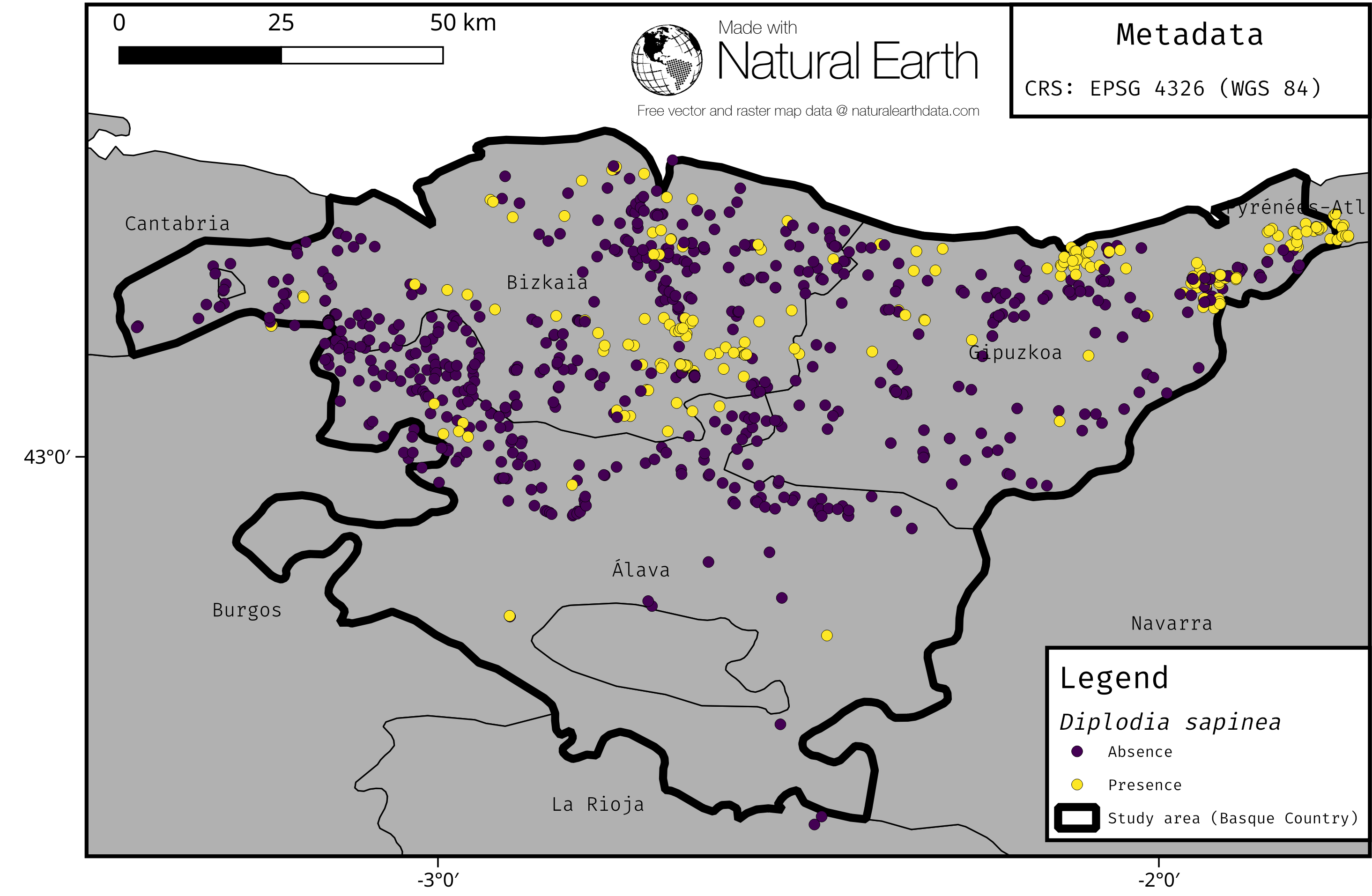 .font70[**Fig. 2:** Study area (Basque Country, Spain)] ] --- class: inverse, center, middle # Methods <i class="fa fa-cogs"></i> <html><div style='float:left'></div><hr color='#EB811B' size=1px width=720px></html> --- # Methods <i class="fa fa-cogs"></i> ## Machine-learning models * Boosted Regression Trees (`BRT`) * Random Forest (`RF`) * Support Vector Machine (`SVM`) * k-nearest Neighbor (`KNN`) ## Parametric models * Generalized Addtitive Model (`GAM`) * Generalized Linear Model (`GLM`) ## Performance Measure Brier Score --- # Methods <i class="fa fa-cogs"></i> ## Nested Cross-Validation * Cross-validation for **performance estimation** * Cross-validation for **hyperparameter tuning** (sequential based model optimization) Different sampling strategies (Performance estimation/Tuning): * Non-Spatial/Non-Spatial * Spatial/Non-Spatial * Spatial/Spatial * Non-Spatial/No Tuning * Spatial/No Tuning --- # Methods <i class="fa fa-cogs"></i> ## Nested (spatial) cross-validation .center[ 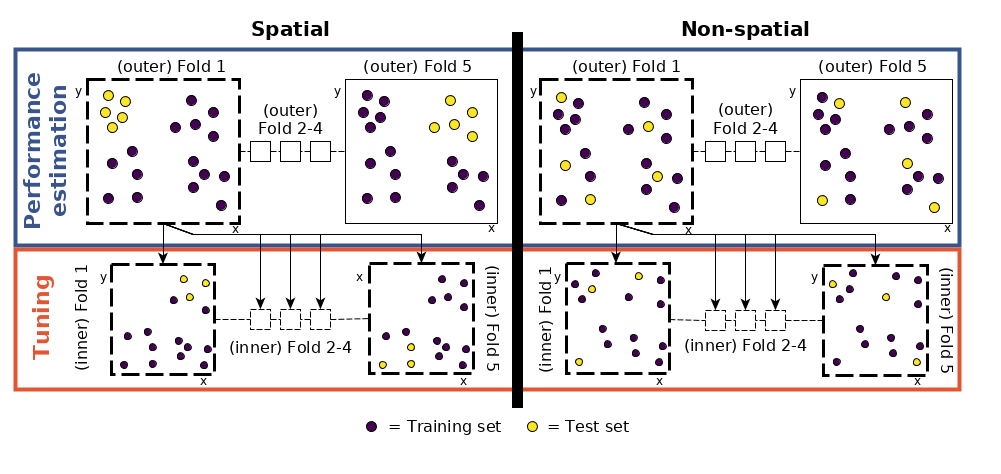 .font70[**Fig. 3:** Nested spatial/non-spatial cross-validation]] --- # Methods <i class="fa fa-cogs"></i> ## Nested (spatial) cross-validation <br> .center[ 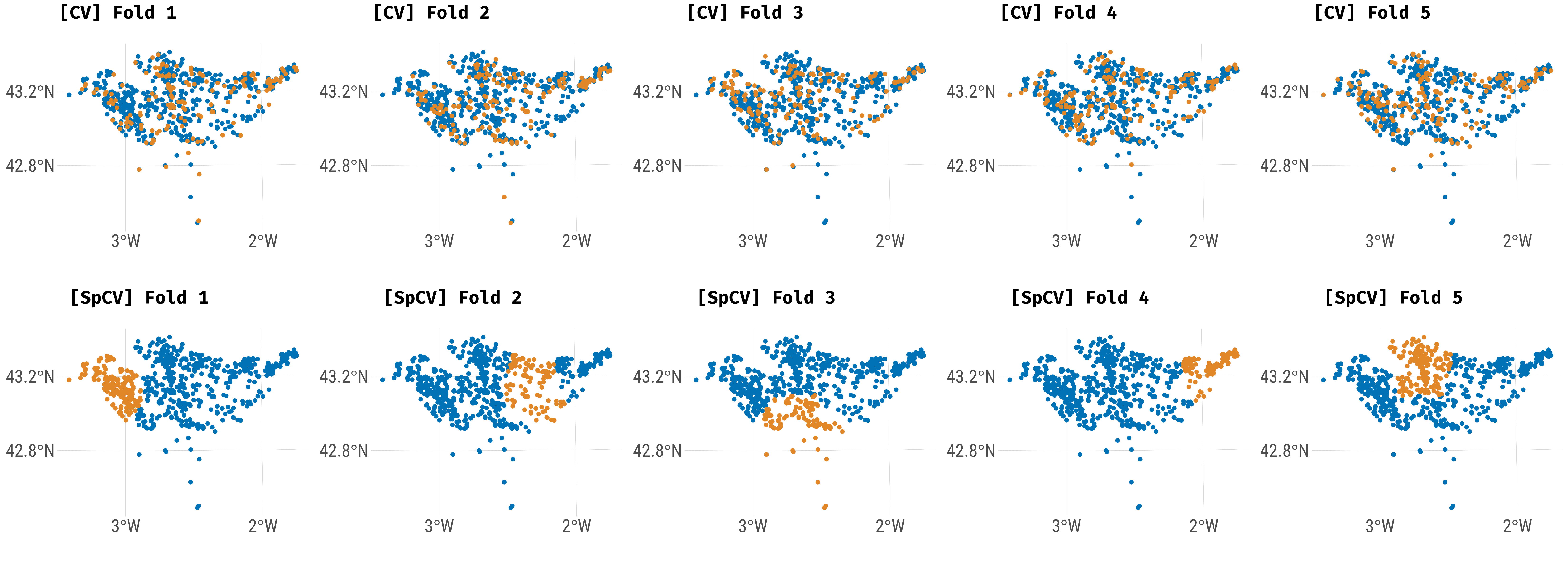 .font70[**Fig. 4:** Comparison of spatial and non-spatial partitioning of the data set.] ] --- # Methods <i class="fa fa-cogs"></i> #### Hyperparameter tuning search spaces RF : [Probst, Wright, and Boulesteix (2018)](#bib-Probst2018b) BRT, SVM, KNN: Self-defined limits based on evaluation of estimated hyperparameters .center[ 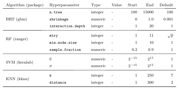 .font70[**Table 1:** Hyperparameter limits and types of each model. Notations of hyperparameters from the respective R packages were used. `\(p\)` = Number of variables.] ] --- class: inverse, center, middle # Results <i class="fa fa-image"></i> <html><div style='float:left'></div><hr color='#EB811B' size=1px width=720px></html> --- # Results <i class="fa fa-image"></i> ## Hyperparameter tuning .center[ 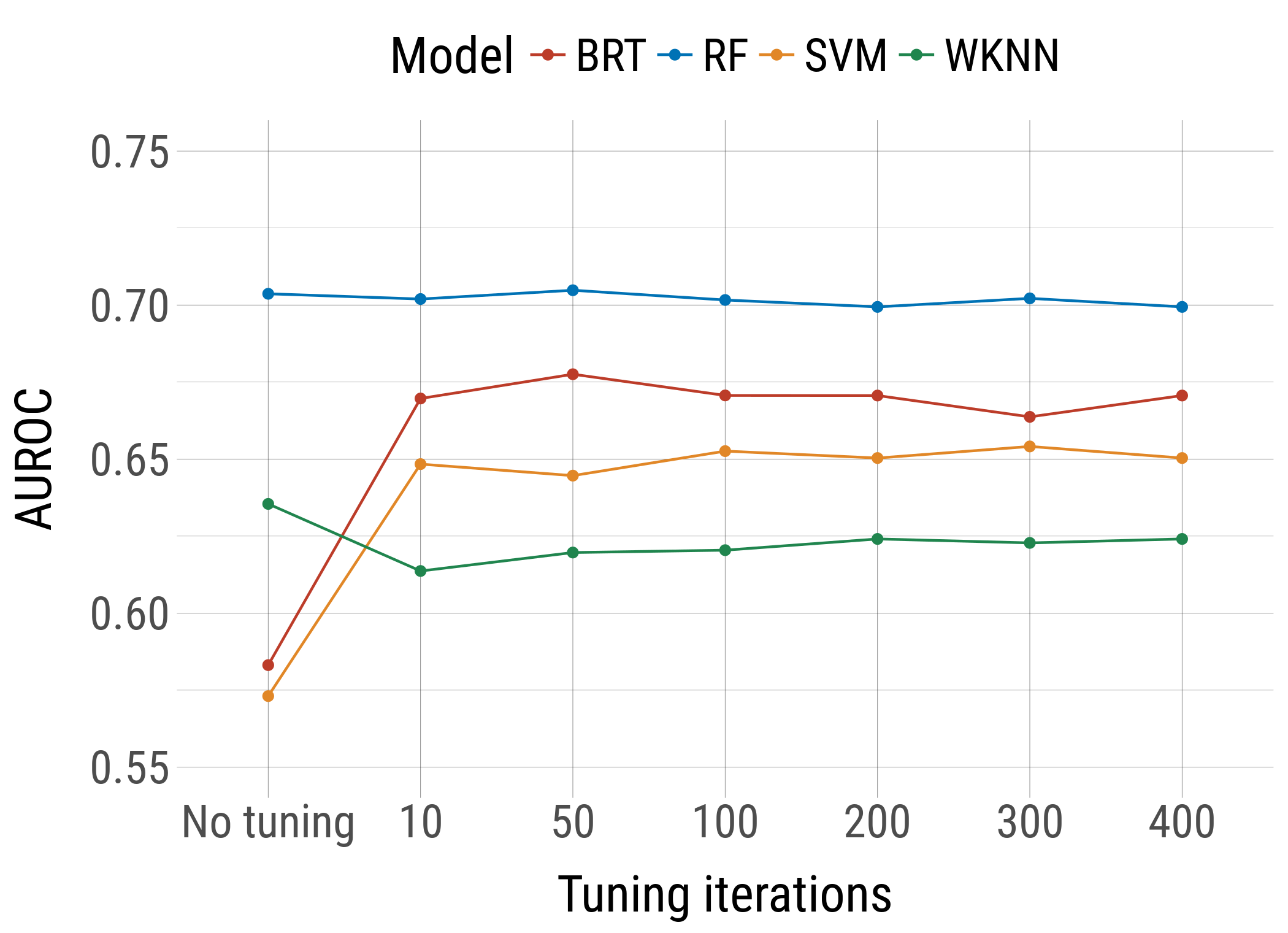 ] .font70[**Fig 4:** Hyperparameter tuning results of the spatial/spatial CV setting for BRT, WKNN, RF and SVM: Number of tuning iterations (1 iteration = 1 random hyperparameter setting) vs. predictive performance (AUROC). ] --- # Results <i class="fa fa-image"></i> (Predictive Performance) .center[ 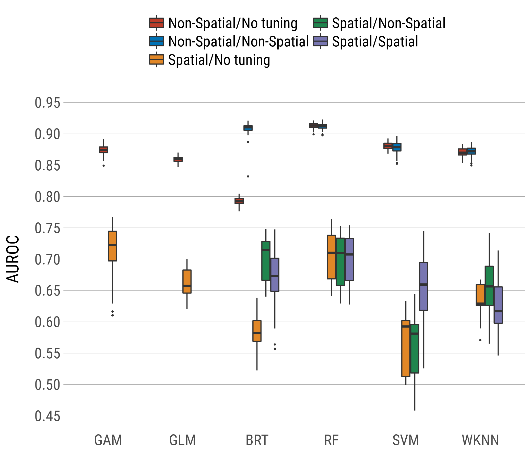 ] .font70[**Fig 5:** (Nested) CV estimates of model performance at the repetition level using 200 random search iterations. CV setting refers to perfomance estimation/hyperparameter tuning of the respective (nested) CV, e.g. ”Spatial/Non-Spatial” means that spatial partitioning was used for performance estimation and non-spatial partitioning for hyperparameter tuning. ] --- class: inverse, center, middle # Discussion <i class="fa fa-comments"></i> <html><div style='float:left'></div><hr color='#EB811B' size=1px width=720px></html> --- # Discussion <i class="fa fa-comments"></i> ## Predictive performance * `RF` and `GAM` showed the best predictive performance <i class="fa fa-trophy"></i> -- * High bias in performance when using non-spatial CV --- # Discussion <i class="fa fa-comments"></i> (Performance) .center[  ] .font70[**Fig 6:** (Nested) CV estimates of model performance at the repetition level using 200 random search iterations. CV setting refers to perfomance estimation/hyperparameter tuning of the respective (nested) CV, e.g. ”Spatial/Non-Spatial” means that spatial partitioning was used for performance estimation and non-spatial partitioning for hyperparameter tuning. ] --- # Discussion <i class="fa fa-comments"></i> ## Predictive Performance * `RF` and `GAM` showed the best predictive performance <i class="fa fa-trophy"></i> * High bias in performance when using non-spatial CV * Parametric models (`GLM`, `GAM`) show equally good performance estimates as the best ML algorithm (`RF`) --- # Discussion <i class="fa fa-comments"></i> ### [Iturritxa et al. (2014)](http://onlinelibrary.wiley.com/doi/10.1111/ppa.12328/abstract) GLM: 0.65 AUROC (without predictor `hail`) GLM: 0.96 AUROC (with predictor `hail`) ### This work GLM: 0.66 AUROC (without predictor `hail_prob`) + slope, pH, lithology, soil GLM: 0.694 (with predictor `hail_prob`) + slope, pH, lithology, soil --- # Discussion <i class="fa fa-comments"></i> ## Hyperparameter tuning * Saturates at 50 repetitions and has a small effect for `SVM` and `BRT` (arbitrary defaults). -- * Almost no effect on predictive performance for WKNN and RF (reasonable defaults). -- * Default hyperparameters of `RF` (and all other learners) are not suitable for spatial data --- # Discussion <i class="fa fa-comments"></i> (Tuning) 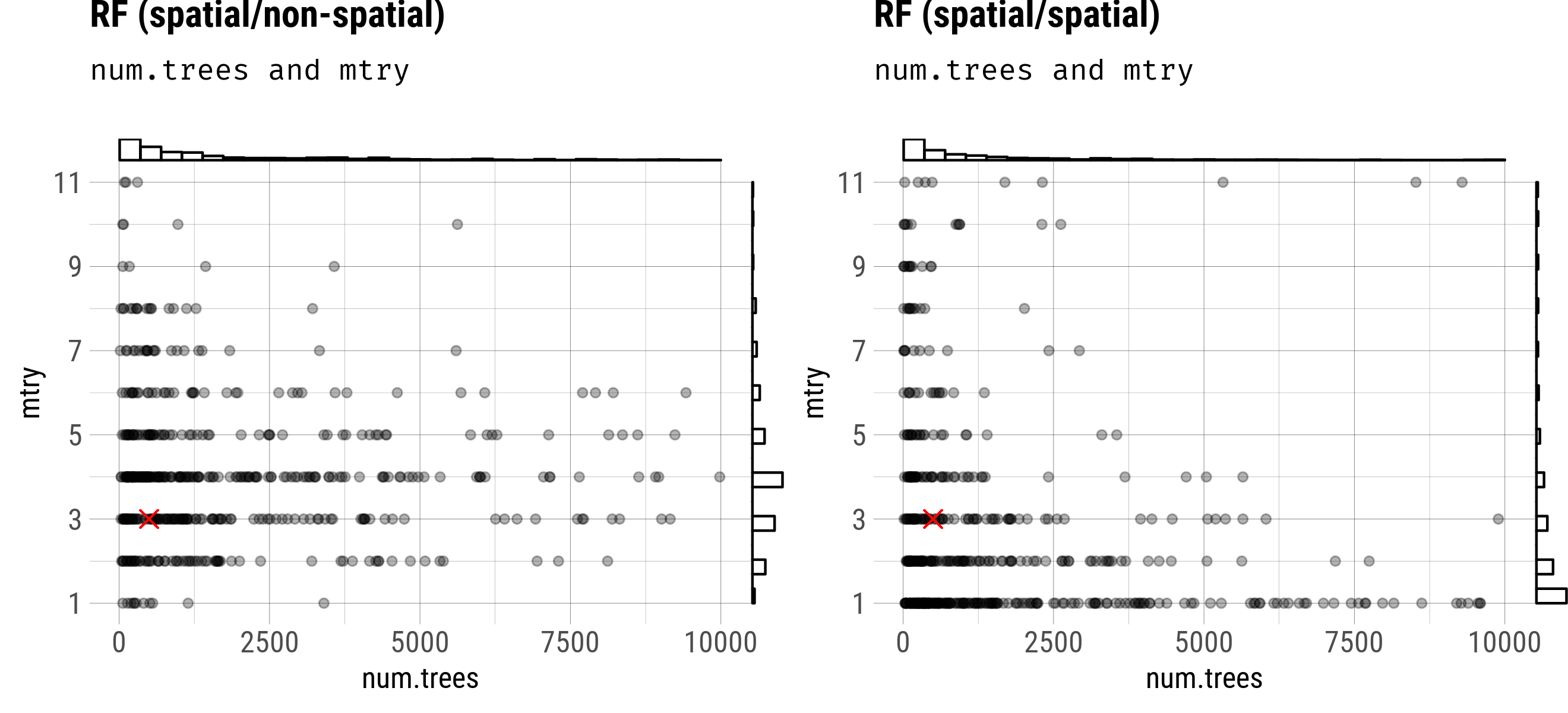 .font70[**Fig 7:** Best hyperparameter settings by fold (500 total) each estimated from 200 random search tuning iterations per fold using five-fold cross-validation. Split by spatial and non-spatial partitioning setup. Red crosses indicate default hyperparameter values. Black dots represent the winning hyperparameter setting out of each random search tuning of the respective fold.] --- # Discussion <i class="fa fa-comments"></i> ## Hyperparameter tuning * Saturates at ~ 50 repetitions and has a small effect for `SVM` and `BRT` (arbitrary defaults). * Almost no effect for `WKNN` and `RF` (reasonable defaults). * Default hyperparameters of `RF` (and all other learners) are not suitable for spatial data * They **possibly** lead to biased performance estimates as they cause fitted models to make use of the remaining spatial autocorrelation in the data. * Meaningful default values (`RF`, `WKNN`) have been estimated on non-spatial data sets. <i class="fa fa-exclamation-circle"></i> Always perform a spatial hyperparameter tuning for spatial data sets, even if it does not improve accuracy <i class="fa fa-exclamation-circle"></i> --- # References <i class="fa fa-copy"></i> <i class="fa fa-file-text-o" aria-hidden="true"></i> Bergstra, J., & Bengio, Y. (2012). Random search for hyperparameter optimization. J. Mach. Learn. Res., 13, 281–305. URL: http://dl.acm.org/citation.cfm?id=2188385.2188395. <i class="fa fa-file-text-o" aria-hidden="true"></i> Iturritxa, E., Mesanza, N., & Brenning, A. (2014). Spatial analysis of the risk of major forest diseases in Monterey pine plantations. Plant Pathology, 64, 880–889. doi:[10.1111/ppa.12328](http://onlinelibrary.wiley.com/doi/10.1111/ppa.12328/abstract). Probst, P, M. Wright and A. Boulesteix (2018). "Hyperparameters and Tuning Strategies for Random Forest". In: _ArXiv e-prints_. arXiv: 1804.03515 [stat.ML]. --- class: inverse, center, middle # Backup <i class="fa fa-plus-square"></i> <html><div style='float:left'></div><hr color='#EB811B' size=1px width=720px></html> --- # Backup <i class="fa fa-plus-square"></i> .center[ 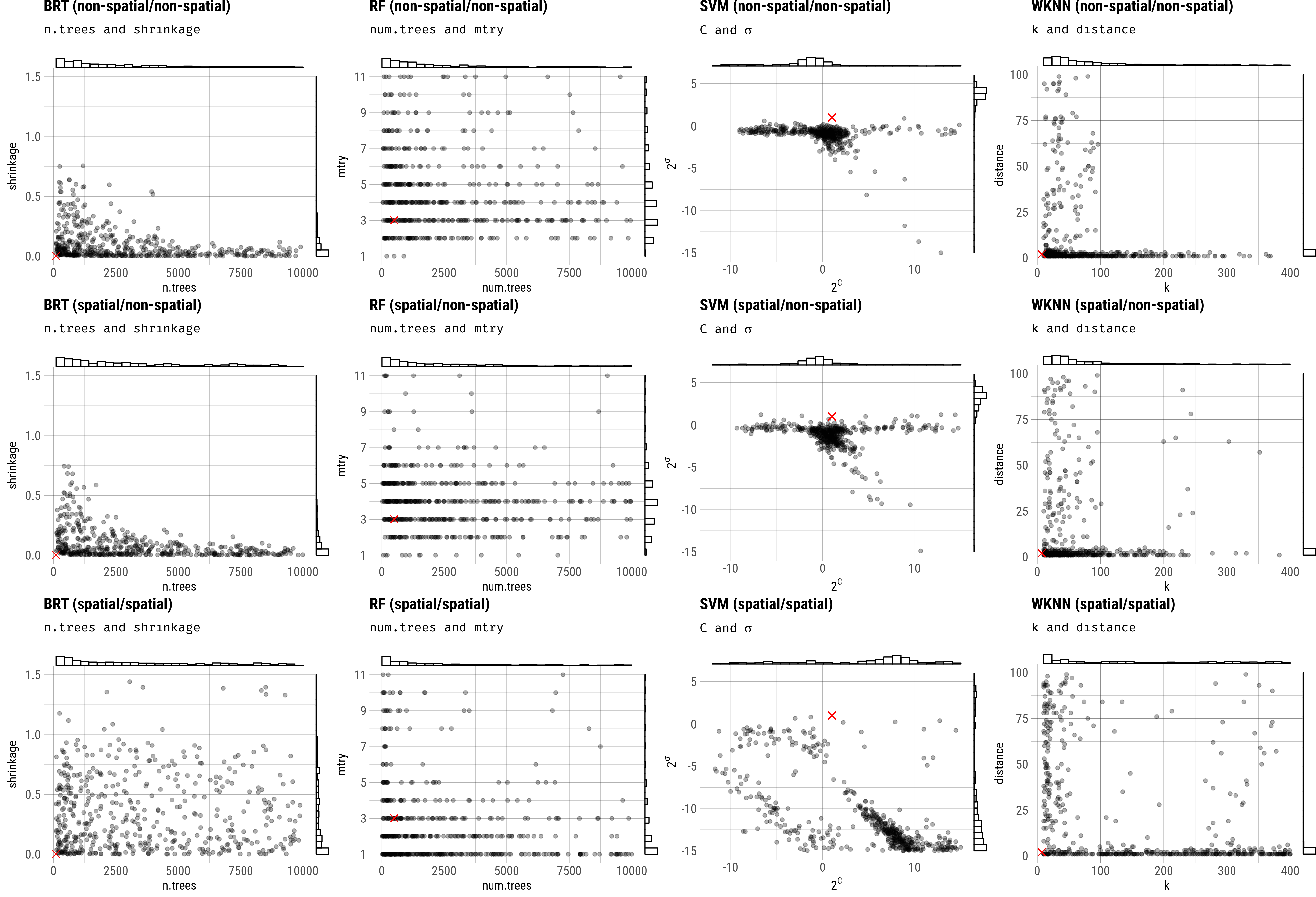 ] --- # Backup <i class="fa fa-plus-square"></i> <br> .center[ 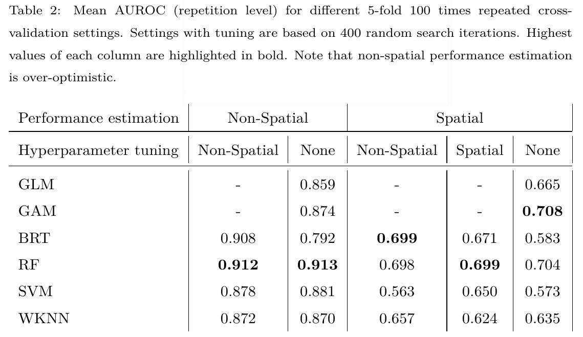 ]