FSU activity report: 03/2017

# FSU activity report: 03/2017 - 12/2017
## <html>
<div style="float:left">

</div>
<hr color='#EB811B' size=1px width=796px>
</html>
### Patrick Schratz, Jannes Muenchow, Marco Pena, Daphne Meyreiss, Alexander Brenning
### LIFE Healthy Forest Meeting, Vitoria, 13 Dec 2017

---

---

# Outline

1) Action A2.1.6: **Acquisition of hyperspectral imagery**

2) Action B1.1: **Spatial mapping using statistical and machine-learning data analysis**

---

# Action A2.1.6: Acquisition of hyperspectral imagery

---

# Acquisition of hyperspectral imagery

## Prior to March 2017

* Hyperspectral imagery was acquired by HAZI in September 2016 for all plots (28 in total)

* Unfortunately, one of the five demonstration plots ("hernani") was not covered by the flight mission

* FSU helped with the planning of the flight routes (Marco Pena)

* Hyperspectral sensors Hyperion-1 was decomissioned in January without prior notice

* Airborne AVIRIS data as a replacement not suitable (price, flights only in US)

* No other spaceborne hyperspectral sensor available

---

# Acquisition of hyperspectral imagery

## March 2017 - Now

We decided to acquire spaceborne multispectral Sentinel-2 data as an alternative for Hyperion-1 data.

**Aim:** Time-series analysis of the vegetation period for 2016 and 2017

## Why time-series analysis?

* Due to the offset in both spatial and radiometric-resolution (1m vs. 10m, 126 bands vs. 10 bands) it is not possible to directly compare multispectral images and hyperspectral images.

* Time-series analysis might reveal changes over time of infested trees by using various indices (e.g. vegetation indices).

* Possible trends can still be post-analysed with hyperspectral imagery from September 2016.

---

# Acquisition of hyperspectral imagery

Acquisition period: 
 * March 2016 - November 2016
 * March 2017 - November 2017
 * Repetition rate: 10 days
 
So far we acquired **391 images** (each 500MB) in total resulting combining to ~ **200GB** of raw data.

For every of the 27 plots we have **135** images. 
These got cropped to the respective plot extent leaving a total of **70 MB** for the complete time-series.
 
**Daphne Meyreiss** (student assistant) was in charge of the processing.

Pre-processing (Download, cropping) of all plots is planned to be finished at the end of 2017.

**Deliverable contributions:**
 * Remotely-sensed forest health map (06/2018) *B1*
 * Integrated analysis of characterization results at large scale (01/2019) *B1*
 * Maps of forest disease potential  (10/2018) *B1*
 
---

# Acquisition of hyperspectral imagery

## Plot "Caranca" with both hyperspectral airborne and multispectral Sentinel-2 image

.pull-left[.center[
Multispectral image (Sentinel-2, 10m)
</br>
![:scale 95%](figs/caranca_sentinel.png)
]]

---

# Action B1.1: Spatial mapping using statistical and machine-learning data analysis

---

# Action B1.1: Spatial mapping

**Analysis goal:** Which model performs best in classifying infested trees (Diplodia Pinea) using environmental variables as predictors?

**Predictors:** Temperature, precipitation, tree age, soil type, lithology type, pH value, hail damage, elevation, slope

**Related work:** Iturritxa et al. (2014): Spatial analysis of the risk Monterey pine plantations.

This worked analysed the influence of the predictor variables using parametric models (GLM, GAM) while the current analysis compared statistical and machine-learning models focusing on predictive performance.

---

# Action B1.1: Spatial mapping

## Key Points:

* State-of-the-art parametric and non-parametric models (BRT, GAM, GLM, KNN, RF, SVM)

* Accounting for spatial autocorrelation by using bias-reduced **spatial cross-validation**

* Extensive **hyperparameter tuning** of machine-learning models to ensure best possible performance results

\>>> "How-to" guide for bias-reduced spatial model comparison analysis.

---

# Action B1.1: Spatial mapping

## Performance results

---

# Action B1.1: Spatial mapping

## Exemplary hyperparameter tuning result

---

# Action B1.1: Spatial mapping

## Runtime comparison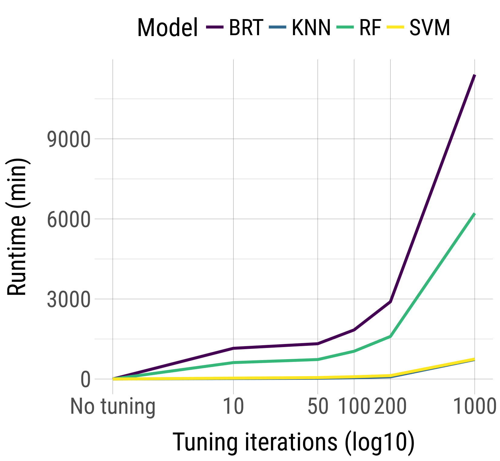

---

# Action B1.1: Spatial mapping

## Ridge regression analysis of hyperspectral data

**Goal:** Find vegetations indices which reveal a pattern in defoliation of infested trees

**Approach:** Calculate all possible vegetation indices + narrow band indices ( `\(\frac{B1 + B2}{B1 - B2)}\)` ) on different resolutions (1m - 5m). 
This results in a data set with 30k+ variables which are modelled using ridge regression (M. Pena).

**Data sets**: Demonstration plots (Laukiz I, Laukiz II, Oiartzun, Luiando)

---

# Action B1.1: Spatial mapping

## Ridge regression analysis of hyperspectral data

Pearson’s correlation coefficient between more than 30.000 indices and the observed defoliation in the field (Laukiz I)

---

# Action B1.1: Spatial mapping

## Ridge regression analysis of hyperspectral data

.center[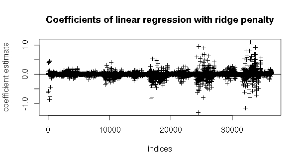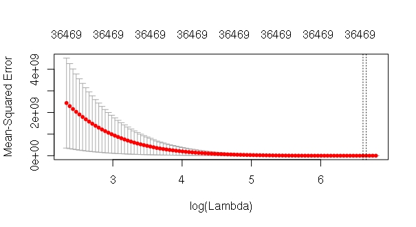
![:scale 50%](figs/Laukiz2_coeff_ridge_penalty.jpeg)
![:scale 50%](figs/Laukiz2_lambda_plot.jpeg)

]

---

# Action B1.1: Spatial mapping

## Milestone and deliverable contributions

* Guide with the identification and characterization of invasive and pathogenic agents (10/2018) *B1* *Deliverable*

* Integrated analysis of characterization results at large scale (01/2019) *B1* *Deliverable*

* Developed model of forest disease potential (10/2018) *B1* *Milestone*

* Data for spatial analysis compiled (10/2018) *B1* *Milestone*

* Final selection of algorithm for remotely-sensed forest health mapping (10/2018) *B1* *Milestone*

* Design and study of algorithms (10/2018) *B3* *Milestone*

---

# Outlook

---

# Outlook

* Modeling of pathogen **Armillaria** using environmental variables as predictors and utilizing the winning algorithm of the model comparison analysis (Random Forest)

* Model comparison analysis of **defoliation** using hyperspectral indices as predictors including hyperparameter tuning

* Time-series analysis of acquired **Sentinel-2 data**

* Analysis of **new in-situ data** acquired by NEIKER in October 2017 (received this week)