![]()
![]()
2. Linear algebra
2.1. Motivation
We are able to solve equations of the form: $ax + b = c$, where $a,b,c$ are real coefficients and $x$ is the unknown variable.
For example we can follow the next steps to solve the $5x + 3 = 13$ equation
$$\begin{align*} 5x + 3 &= 13 \quad | -3\\ 5x &= 10 \quad | : 5\\ x &= 2\\ \end{align*}$$or equivalently
$$\begin{align*} 5x + 3 &= 13 \quad | +(-3)\\ 5x &= 10 \quad | \cdot 5^{-1}= \frac{1}{5}\\ x &= 2\\ \end{align*}$$Let us consider the following set-up. You have beakfast together with some of your colleagues and you are paying by turn. You don't know the price of each ordered item, but you remember what was ordered on the previous three days and how much did your colleagues pay for it each time:
- 3 days ago your group has ordered 5 croissants, 4 coffees and 3 juices and they have payed 32.3 CHF.
- 2 days ago your group has ordered 4 croissant, 5 coffees and 3 juices and they payed 32.5 CHF.
- 1 day ago the group has ordered 6 croissants, 5 coffees and 2 juices and that costed 31 CHF.
Today the group has ordered 7 croissants, 4 coffees and 2 juices and you would like to know whether the amount of 35 CHF available on your uni card will cover the consumption or you need to recharge it before paying.
By introducing the notations
- $x_1$ for the price of a croissant,
- $x_2$ for the price of a coffee,
- $x_3$ for the price of a juice,
then our information about the consumption of the previous 3 days can be summarised in the form of the following 3 linear equations
$$\left\{\begin{align} &5\cdot x_1 + 4 \cdot x_2 + 3 \cdot x_3 = 32.3 \\ &4\cdot x_1 + 5 \cdot x_2 + 3 \cdot x_3 = 32.5 \\ &6\cdot x_1 + 5 \cdot x_2 + 2 \cdot x_3 = 31 \end{align}\right.$$
The quantity ordered on the current day is $7\cdot x_1 + 4 \cdot x_2 + 2 \cdot x_3$. To determine this one possibility is to calculate the price of each product separately, i.e. we solve the linear equation system first and then susbstitute the prices in the previous formula.
The above system in matrix form
$$
\left(\begin{array}{ccc}
5 & 4 & 3\\
4 & 5 & 3\\
6 & 5 & 2
\end{array}
\right)\cdot \left(\begin{array}{c}
x_1\\
x_2\\
x_3
\end{array}
\right) =
\left(\begin{array}{c}
32.3\\
32.5\\
31
\end{array}
\right)$$
If we introduce for the matrix, respectively the two vectors in the above formula the notations $A, x, b$, then we get
$$A \cdot x = b$$
One can observe that formally this looks the same as the middle state of our introductory linear equation with real coefficients $5x = 10$. So our goal is to perform a similar operation as there, namely we are looking for teh operation that would make $A$ dissappear from the left hand side of the equation. We will see later that this operation will be the inverse operation of multiplication by a matrix, namely multiplication by the inverse of a matrix.
In our applications we will encounter for example when deriving the weights of the multivariate linear regression, a matrix equation of the form: $A \cdot x + b = 0$. This example motivates the introduction of vector substraction, as well.
2.2. Vectors
Definition of vectors
Vectors are elements of a linear vector space. The vector space we are going to work with is $\mathbb{R}^n$, where $n$ is the dimension of the space and it can be $1, 2, 3, 4, ...$. An element of such a vector space can be described by an ordered list of $n$ components of the vector.
$x = (x_1, x_2, \ldots, x_n)$, where $x_1, x_2,\ldots,x_n \in \mathbb{R}$ is an element of $\mathbb{R}^n$.
Example
2.2.1. Geometrical representation of vectors
Below a 2-dimensional vector is represented. You can move its endpoints on the grid and you will see how do its components change.
from IPython.display import IFrame

IFrame("https://www.geogebra.org/classic/cnvxpycc", 800, 600)
Experiment with the 3-dimensional vector in the interactive window below.
IFrame("https://www.geogebra.org/classic/meg4scuj", 800, 600)
The following interactive window explains when are two vectors equal.
IFrame("https://www.geogebra.org/classic/fkkbkvuj", 800, 600)
2.2.2. Vector addition
Definition of vector addition
Vector addition happens component-wise, namely the sum of the vectors $x = (x_1, x_2, \cdots, x_n)$ and $y = (y_1, y_2, \cdots, y_n)$ is:
$$x+y = (x_1 + y_1, x_2+y_2, \ldots, x_n+y_n)$$There exist two approaches to visualise vector addition
- parallelogram method
- triangle method
Both are visualised below.
IFrame("https://www.geogebra.org/classic/jnchvrhg", 800, 600)
Below you can see another approach to vector addition.
IFrame("https://www.geogebra.org/classic/mzgchv22", 1200, 600)
2.2.3. Multiplication of vectors by a scalar
Definition of the multiplication by a scalar
This happens also component-wise exactly as addition, namely $$\lambda (x_1, x_2, \ldots, x_n) = (\lambda x_1, \lambda x_2, \ldots, \lambda x_n).$$
This operation is illustrated below
IFrame("https://www.geogebra.org/classic/gxhsev8k", 800, 800)
2.2.4. Vector substraction
Definition of vector substraction
Vector substraction happens component-wise, namely the difference of the vectors $x = (x_1, x_2, \cdots, x_n)$ and $y = (y_1, y_2, \cdots, y_n)$ is:
$$x-y = (x_1 - y_1, x_2 - y_2, \ldots, x_n -y_n)$$Observe that vector substraction is not commutative, i.e. $x-y \neq y-x$ in general.
2.2.5. Abstract linear algebra terminology
For any two elements $x,y \in \mathbb{R}^n$ it holds that $$x+y \in \mathbb{R}^n.$$ This property is called closedness of $\mathbb{R}^n$ w.r.t. addition.
Observe the commutativity of the addition on $\mathbb{R}^n$ is inherited by the vectors in $\mathbb{R}^n$, i.e. $$x + y = y + x$$ for any $x, y \in \mathbb{R}^n$.
Observe that addition is also associative on $\mathbb{R}^n$, i.e. $$x + (y + z) = (x + y) + z, \quad \mbox{ for any } x,y,z \in \mathbb{R}^n$$
If we add the zero vector $\mathbf{0} = (0, 0, ..., 0) \in \mathbb{R}^n$ to any other vector $x \in \mathbb{R}^n$ it holds that $$\mathbf{0} + x = x + \mathbf{0} = x.$$ The single element with the above property is called the neutral element w.r.t. addition.
For a vector $x = (x_1, x_2, \ldots, x_n)$ the vector $x^*$ for which $$x + x^* = x^* + x = \mathbf{0}$$ is called the inverse vector of $x$ w.r.t. addition.
What is the inverse of the vector $x = (2, 3, -1)$? Inverse: $-x = (-2,-3,1)$
What is the inverse of a vector $x = (x_1, x_2, \ldots, x_n)$? Inverse: $-x = (-x_1, -x_2, \ldots, -x_n)$
As every vector of $\mathbb{R}^n$ possesses an inverse, we introduce the notation $-x$ for its inverse w.r.t addition.
A set $V$ with an operation $\circ$ that satsifies the above properties is called a commutative or Abelian group in linear algebra. For us $V = \mathbb{R}^n$ and $\circ = +$.
The scalar mutiplication, that we have introduced, has the following properties
- associativity of multiplication: $(\lambda_1\lambda_2) x = \lambda_1 (\lambda_2x)$,
- distributivity: $(\lambda_1 + \lambda_2) x = \lambda_1 x + \lambda_2 x$ and $\lambda(x+y) = \lambda x + \lambda y$,
- unitarity: $1 x = x$, for all $x,y \in \mathbb{R}^n$ and $\lambda, \lambda_1, \lambda_2$ scalars.
Our scalars are elements of $\mathbb{R}$. This set is a field, i.e. the operations $\lambda_1+\lambda_2$, $\lambda_1-\lambda_2$, $\lambda_1\cdot\lambda_2$ make sense for any $\lambda_1, \lambda_2 \in \mathbb{R}$ and the $\lambda_1/\lambda_2 = \lambda_1 \cdot \lambda_2^{-1}$ can be performed also when $\lambda_2 \neq 0$.
A vector space consists of a set $V$ and a field $F$ and two operations:
- an operation called vector addition that takes two vectors $v,w \in V$, and produces a third vector, written $v+w \in V$,
- an operation called scalar multiplication that takes a scalar $\lambda \in F$ and a vector $v\in V$, and produces a new vector, written $cv \in V$, which satisfy all the properties enlisted above (5+3).
Remark
Observe that
$$x-y = x+(-y),$$
which means that the difference of $x$ and $y$ can be visualised as a vector addition of $x$ and $-y$.
$-y$ is here the inverse of the vector $y$ w.r.t. addition. Geometrically $-y$ can be represented by the same oriented segment as $y$, just with opposite orientation.
2.2.6. Modulus of a vector, length of a vector, size of a vector
The length of a vector or norm of a vector $x = (x_1, x_2, \cdots, x_n)$ is given by the formula $$||x|| = \sqrt{x_1^2 + x_2^2 + \cdots x_n^2}$$
Experiment with the interactive window below and derive the missing formula.
IFrame("https://www.geogebra.org/classic/mfzdes3n", 800, 600)
Each vector $x = (x_1, x_2, \ldots, x_n) \in \mathbb{R}^n$ is uniquely determined by the following two features:
- its magnitude / length / size / norm: $r(x) = ||x|| = \sqrt{x_1^2 + x_2^2 + \cdots +x_n^2}$,
- its direction: $e(x) = \frac{x}{||x||} = \frac{1}{\sqrt{x_1^2 + x_2^2 + \cdots +x_n^2}}(x_1, x_2, \ldots, x_n)$.
If the maginute $r \in \mathbb{R}$ and the direction $e \in \mathbb{R}^n$ of a vector is given, then this vector can be written as $re$.
Observe that $\frac{x}{||x||}$ has length $1$.
2.2.7. Dot product / inner product / scalar product
Definition of the dot product
The dot product / inner product / scalar product of two vectors $x = (x_1, x_2)$ and $y = (y_1, y_2)$ is denoted by $\langle x, y\rangle$ and it is equal to the scalar $x_1\cdot y_1+ x_2 \cdot y_2$.
This can be generalised to the vectors $x = (x_1, x_2, \cdots, x_n) \in \mathbb{R}^n$ and $y = (y_1, y_2, \cdots, y_n) \in \mathbb{R}^n$ as $\langle x, y\rangle = x_1\cdot y_1 + x_2 \cdot y_2 + \cdots + x_n\cdot y_n$.
Observe that as a consequence of the definition distributivity over addition holds, i.e. $\langle x , y + z\rangle = \langle x , y \rangle + \langle x , z \rangle$.
Furthermore $\lambda \langle x , y\rangle = \lambda \langle x, y\rangle = \langle x , \lambda y\rangle $.
The last two properties together are called also bilinearity of the scalar product.
Observe also that the scalar product is commutative, i.e. $\langle x, y\rangle = \langle y, x \rangle$.
Question: What's the relation between the length of a vector and the dot product?
Length of a vector: $||x|| = \sqrt{x_1^2+x_2^2 + \cdots x_n^2}$
The dot product of two vectors: $\langle x , y \rangle= x_1\cdot y_1 + x_2 \cdot y_2 + \cdots + x_n\cdot y_n$.
Substituting $x$ in the last equation instead of $y$, we obtain
$$\mathbf{\langle x , x \rangle} = x_1^2+x_2^2 + \cdots x_n^2 = \mathbf{||x||^2}$$Convention
When talking exclusively about vectors, for the simplicity of writing, we often think of them as row vectors. However, when matrices appear in the same context and there is a chance that we will multiply a matrix by a vector, it is important to specify also whether we talk about a row or column vector. In this extended context a vector is considered to be a column vector by default.
From now on we are going to follow also this convention and we are going to think of a vector always as a column vector.
Relationship of dot product and matrix multiplication
Even if we didn't define formally the matrix product yet, we mention its relationship with the dot product, because in mathematical formulas it proves to be handy to have an alternative way for writing the dot multiplication.
The following holds for any vectors $x,y \in \mathbb{R}^n$ $$\mathbf{\langle x,y \rangle} = x_1\cdot y_1 + x_2 \cdot y_2 + \cdots x_n \cdot y_n = (\begin{array}{cccc} x_1 & x_2 & \ldots & x_n \end{array})\cdot\left(\begin{array}{c} y_1\\ y_2\\ \vdots\\ y_n \end{array}\right) = \mathbf{x^T \cdot y},$$ where $\mathbf{x^T \cdot y}$ denotes the matrix product of the row vector $x_T$ and the column vector $y$.
Furthermore, observe that due to the commutativity of the dot product
$$x^T \cdot y = \langle x, y \rangle = \langle y, x\rangle = y^T \cdot x$$
2.2.8. The dot product and the cosine rule
Let us consider two vectors $u$ and $d$ and denote their angle by $\theta$. We construct the triangle having as sides the vectors $u$, $d$ and $u-d$. In the forthcoming we derive the formula $$\langle u, d \rangle = ||u||\cdot ||d||\cdot cos(\theta)$$ from the law of cosines.
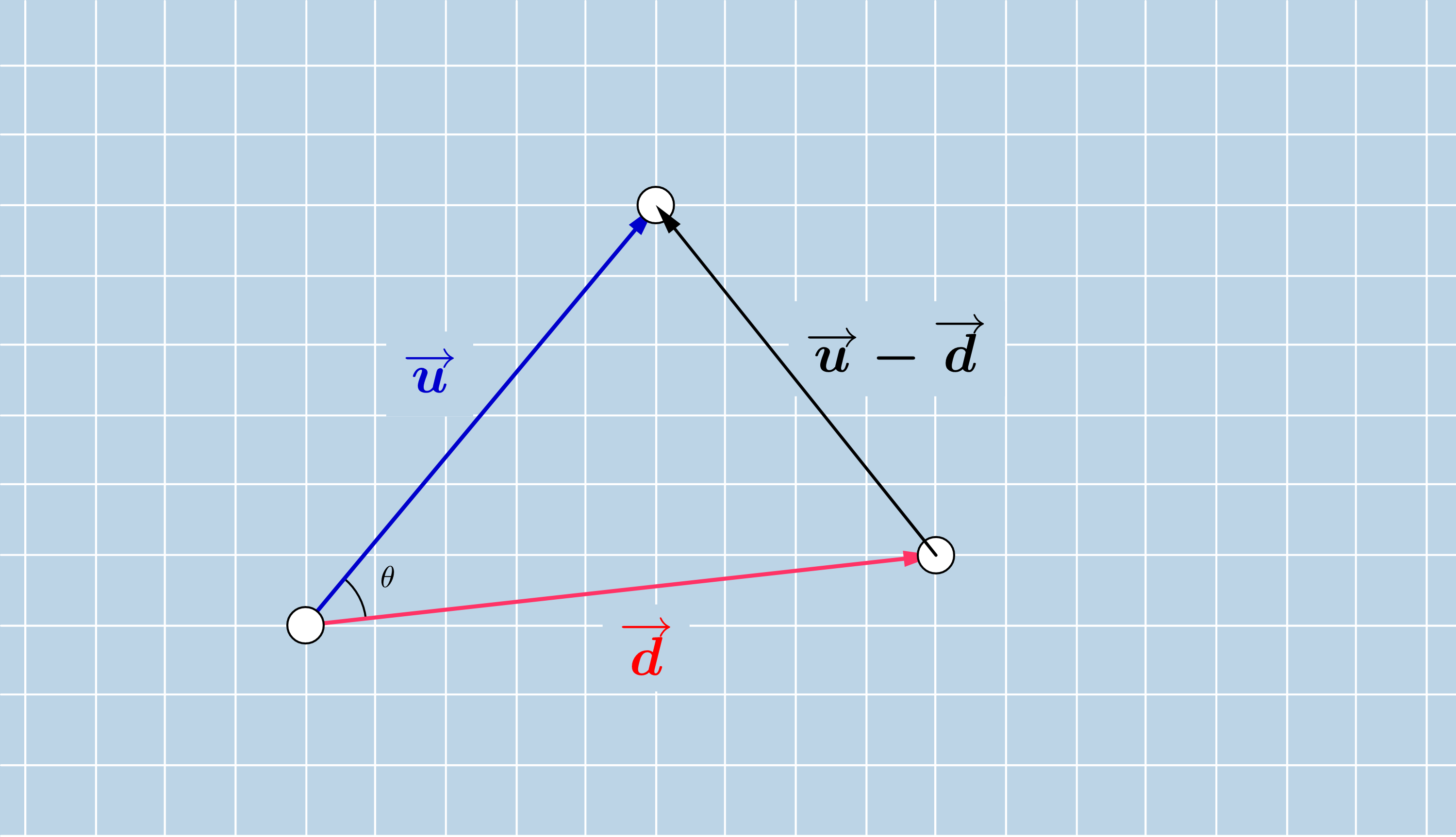
The law of cosines is a generalisation of the Pythagorean theorem in a triangle, which holds not just for right triangles. As the Pythagorean theorem, this formulates also a relationship between the lengths of the three sides. In a triangle with side lengths $a$, $b$ and $c$ and an angle $\theta$ opposite to the side with length $a$, the law of cosines claimes that
In our setting we can write for the side lengths the norm / length of the vectors $u$, $d$, respectively $u-d$. In this way we obtain
On the other hand using the relationship between the length of a vector and the dot product, we can write the following
Using the bilinearity and commutativity of the dot product we can continue by
$$\begin{align*}
||u-d||^2 = \langle u-d,u-d \rangle = \langle u, u\rangle - \langle d,u \rangle - \langle u,d \rangle - \langle d, d \rangle = ||u||^2 + ||d||^2- 2\langle d,u \rangle
\end{align*}$$
Summing up what did we obtain until now
$$\left\{
\begin{align*}
||u-d||^2 = ||u||^2 + ||d||^2 - 2\cdot||u||\cdot ||d||\cdot\cos(\theta)\\
||u-d||^2 = ||u||^2 + ||d||^2- 2\langle d,u \rangle
\end{align*}
\quad \right|
\Rightarrow \quad
||u||^2 + ||d||^2 - 2\cdot||u||\cdot ||d||\cdot\cos(\theta) = ||u||^2 + ||d||^2- 2\langle d,u \rangle
$$
or equivalently
$$ ||u||\cdot ||d||\cdot\cos(\theta) = \langle u,d \rangle$$
Observe that from the above cosine rule one can express $\cos(\theta)$ of the vectors $u$ and $d$ as
$$\cos(\theta) = \frac{\langle u, d\rangle }{||u|| \cdot ||d||}$$2.2.9. Scalar and vector projection
Scalar projection: length of the resulting projection vector, namely
where $\theta$ is the angle of the vectors $d$ and $u$.
Due the cosine rule that we have derived for the scalar product, we can substitute $\cos(\theta)$ by $\frac{\langle d,u\rangle}{||u|| \cdot ||d||}$ and we obtain the following formula for the length of the projection
$$||\pi_d(u)|| = \frac{\langle u, d \rangle}{||u|| \cdot ||d||} \cdot ||u|| = \frac{\langle u,d \rangle}{||d||}$$Vector projection: We have determined the magnite of the projection vector, the direction is given by the one of the vector $d$. These two characteristics do uniquely define the projection vector, thus we can write
$$\pi_d(u) = ||\pi_d(u)|| \frac{d}{||d||}= \mathbf{\frac{\langle u, d\rangle }{||d||} \frac{d}{||d||}} = \frac{d \langle u, d\rangle}{||d||^2} = \frac{d \langle d, u\rangle}{||d||^2}= \frac{d \cdot (d^T \cdot u)}{||d||^2}= \frac{(d \cdot d^T) \cdot u}{||d||^2} = \mathbf{\frac{d \cdot d^T}{||d||^2}\cdot u}$$The projection matrix $\frac{d \cdot d^T}{||d||^2}$ in $\mathbb{R}^n$ is an $n \times n$-dimensional matrix.
IFrame("https://www.geogebra.org/classic/qhhqpmrt", 1000, 600)
2.2.10. Quiz
Question 1
What is the dot product / scalar product of the vectors $x$ and $y$ given below?
$$\mbox{a) } x = \left( \begin{array}{c} 1\\ 2 \end{array} \right),\ y = \left( \begin{array}{c} 3\\ -2 \end{array} \right)$$$$\mbox{b) } x = \left( \begin{array}{c} 1\\ 2\\ -1 \end{array} \right),\ y = \left( \begin{array}{c} 3\\ -2\\ -1 \end{array} \right)$$Question 2
What is the length of the vectors $u = \left( \begin{array}{c} 4\\ 3 \end{array} \right)$ and $v = \left( \begin{array}{c} 1\\ 0\\ -1 \end{array} \right)$?
Question 3
What is the angle of the vectors $x$ and $y$ given below?
$$\mbox{a) } x = \left( \begin{array}{c} 2\\ 3\\ 2 \end{array} \right), y = \left( \begin{array}{c} 1\\ 0\\ -1 \end{array} \right)$$$$\mbox{b) } x = \left( \begin{array}{c} \sqrt{3}\\ 1 \end{array} \right), y = \left( \begin{array}{c} -\sqrt{2}/2\\ \sqrt{2}/2 \end{array} \right)$$Question 4
What is the length of the projection of vector $x$ to vector $y$, where $x$ and $y$ are the vectors from the previous question.
Question 5
Caculate the vector projection $\pi_u(x)$, where $u$ and $x$ are given as follows?
$$\mbox{a) } u = \left( \begin{array}{c} 1\\ 2 \end{array} \right),\ x = \left( \begin{array}{c} 3\\ -2 \end{array} \right)$$$$\mbox{b) } u = \left( \begin{array}{c} 1\\ 2\\ -1 \end{array} \right),\ x = \left( \begin{array}{c} 3\\ -2\\ -7 \end{array} \right)$$#from ipywidgets import widgets, Layout, Box, GridspecLayout
#from File4MCQ import create_multipleChoice_widget
#test = create_multipleChoice_widget("1. Question: What day of the week is it today the 1st of September 2020?", ['a. Monday', 'b. Tuesday', 'c. Wednesday'],'b. Tuesday','[Hint]:')
#test
2.2.11. Basis of a vectorspace
Definition of linear combination
A linear combination of the vectors $x^{(1)}, x^{(2)}, \ldots, x^{(m)} \in \mathbb{R}^n$ is a vector of $\mathbb{R}^n$, which can be written in the form of
$$\lambda_1x^{(1)} + \lambda_2 x^{(2)} + \cdots \lambda_m \cdot x^{(m)},$$where $\lambda_1, \lambda_2, \ldots, \lambda_m$ are real valued coefficients.
Example
Consider the vectors $x^{(1)} = \left( \begin{array}{c} 1 \\ 0\\ 2 \end{array} \right)$ and $x^{(2)} = \left( \begin{array}{c} 0 \\ 1\\ 0 \end{array} \right).$
Then
$$2 x^{(1)} + 3x^{(2)}= 2\left( \begin{array}{c} 1 \\ 0\\ 2 \end{array} \right) + 3 \left( \begin{array}{c} 0 \\ 1\\ 0 \end{array} \right) = \left( \begin{array}{c} 2 \\ 3\\ 4 \end{array} \right)$$is a linear combination of $x^{(1)}$ and $x^{(2)}$.
Definition of linear dependence
Let us consider a set of $m$ vectors $x^{(1)}, x^{(2)}, \ldots, x^{(m)}$ in $\mathbb{R}^n$. They are said to be linearly dependent if and only if there exist the not all zero factors $\lambda_1, \lambda_2, \ldots, \lambda_m \in \mathbb{R}$ such that
Remark
Observe that if $x^{(1)}, x^{(2)}, \ldots, x^{(m)}$ are dependent, then for some not all zero factors $\lambda_1, \lambda_2, \ldots, \lambda_m \in \mathbb{R}$ it holds that
We know that at least one of the factors is not zero, let us assume that $\lambda_i$ is such a factor. This means that from the above equation we can express the vector $x_i$ as a linear combination of the others.
Definition of linear independence
$m$ vectors $x^{(1)}, x^{(2)}, \ldots, x^{(m)}$ in $\mathbb{R}^n$ are linearly independent if there exist no such factors $\lambda_1, \lambda_2, \ldots, \lambda_m \in \mathbb{R}$ for which
and where at least one factor is different of zero.
Alternative definition of linear independence
Equivalently $x^{(1)}, x^{(2)}, \ldots, x^{(m)}$ in $\mathbb{R}^n$ are linearly independent if and only if the equation
holds just for $\lambda_1 = \lambda_2 = \cdots = \lambda_m = 0.$
Remark
If we write the vectors from the above equation by their components, the above equation can be equivalently transformed to
In the process of the above transformation we used tacitly the definition of the matrix product.
Definition of generator set / spanning set
Let us consider the set of vectors $S = \{x^{(1)}, x^{(2)}, \ldots, x^{(m)}\}$ in a vector space $V$ over a field $F$. $S$ is said to be a generator set of the vectors space $V$ if
that is every element of the vector space $V$ can be written a linear combination of the vectors $x^{(1)}, x^{(2)}, \ldots, x^{(m)}$.
Remark
The set of all linear combinations that can be formed from the elements of $S$: $\{\lambda_1x^{(1)} + \lambda_2 x^{(2)} + \cdots +\lambda_m x^{(m)}| \lambda_1, \lambda_2, \ldots, \lambda_m \in F\}$, is denoted by ${\rm span}(S)$.
Remark
With the help of the new notion of spanning set we can give an equivalent definition for linear dependence and independence of vectors:
- The vectors $x^{(1)}, x^{(2)}, \ldots, x^{(m)} \in \mathbb{R}^n$ are linearly dependent if and only if one of them belongs to the span of the others.
- The vectors $x^{(1)}, x^{(2)}, \ldots, x^{(m)} \in \mathbb{R}^n$ are linearly independent if and only if none of them belongs to the span of the others.
Definition of a basis
The vectors $x^{(1)}, x^{(2)}, \ldots, x^{(m)}$ of a vector space $V$ form a basis of $V$ if
$$\mbox{they are linearly independent}$$$$\mbox{&}$$$$\mbox{they form a generator set for }V$$Remark
If $S =\{x^{(1)}, x^{(2)}, \ldots, x^{(m)}\}$ is a generator set of a vector space $V$ over a field $F$, then each element of the space can be written az linear combination of the elements of $S$. Moreover, if this generator set contains linearly independent vectors, then the coefficients of the linear combination associated to a vector are unique and in this case we call the elements of $S$ a basis.
The fact that $x^{(1)}, x^{(2)}, \ldots, x^{(m)}$ are forming a generator set assures that every vector can be exppressed w.r.t. to the $x^{(1)}, x^{(2)}, \ldots, x^{(m)}$ (as a linear combination of $x^{(1)}, x^{(2)}, \ldots, x^{(m)}$).
The fact that $x^{(1)}, x^{(2)}, \ldots, x^{(m)}$ are linearly independent assures that every vector from their span is uniquely expressed as a linear combination of $x^{(1)}, x^{(2)}, \ldots, x^{(m)}$.
We express our vectors in a basis, because this gives a representation for all vectors and two vectors are equal in this representation if and only if the corresponding coordinates / components of the two vectors are the same.
Remark about the components of a vector and the canonical basis
The canonical basis of the vector space $\mathbb{R}^n$ is given by the vectors
A vector $x = \left( \begin{array}{c} x_1 \\ x_2 \\ \vdots \\ x_n \end{array} \right)$ can be written as the following linear combination of the canonical vectors
$$x = \left( \begin{array}{c} x_1 \\ x_2 \\ \vdots \\ x_n \end{array} \right) = x_1 \left( \begin{array}{c} 1 \\ 0 \\ \vdots \\ 0 \end{array} \right) + x_2 \left( \begin{array}{c} 0 \\ 1 \\ \vdots \\ 0 \end{array} \right) + \cdots + x_n \left( \begin{array}{c} 0 \\ 0 \\ \vdots \\ 1 \end{array} \right) = x_1 e_1 + x_2 e_2 + \cdots + x_n e_n,$$Observe that the components of the vector are exactly the coordinates of the vector in the canonical basis.
Exercise
What are the coordinates of the vector $x = \left(
\begin{array}{c}
1 \\
1
\end{array}
\right)$ in the basis given by the vectors $u = \left(
\begin{array}{c}
4 \\
3
\end{array}
\right)$ and $v = \left(
\begin{array}{c}
-3 \\
4
\end{array}
\right)$?
Can you give a formula suited to calculate the coordinates / components of an arbitrary vector in the new basis of $\mathbb{R}^2$?
2.3. Matrices
Definition of matrices, matrix addition, multiplication by a scalar of matrices
$n \times m$-dimensional matrices are elements of the set $\mathbb{R}^{n \times m}$.
We organise the elements of an $n \times m$-dimensional matrix in $n$ rows and $m$ columns.
For the notation of matrices we use often capital letters of the alphabet.
For a matrix $X \in \mathbb{R}^{n \times m}$ let us denote the element at the intersection of the $i$th row and $j$th column by $x_{i,j}$. Then we can define the matrix by its compenents in the following way
$$X = \left( \begin{array}{cccc} x_{1,1} & x_{1,2} & \cdots & x_{1,m}\\ x_{2,1} & x_{2,2} & \cdots & x_{2,m}\\ \vdots\\ x_{n,1} & x_{n,2} & \cdots & x_{n,m} \end{array} \right)$$Matrix addition and multiplication by a scalar happens component-wise, exactly as in the case of vectors. The sum of the matrices $X = (x_{i,j})_{i=\overline{1,n}, j = \overline{1,m}} \in \mathbb{R}^{n \times m}$ and $Y = (y_{i,j})_{i=\overline{1,n}, j = \overline{1,m}} \in \mathbb{R}^{n \times m}$ is the matrix
$$X+Y = (x_{i,j} + y_{i,j})_{i=\overline{1,n}, j = \overline{1,m}},$$that is
$$X+Y = \left( \begin{array}{cccc} x_{1,1} + y_{1,1} & x_{1,2} + y_{1,2} & \cdots & x_{1,m} + y_{1,m}\\ x_{2,1} + y_{2,1} & x_{2,2} + y_{2,2} & \cdots & x_{2,m} + y_{2,m}\\ \vdots\\ x_{n,1} + y_{n,1} & x_{n,2} + y_{n,2} & \cdots & x_{n,m} + y_{n,m} \end{array} \right)$$For $\lambda \in \mathbb{R}$ and $X = (x_{i,j})_{i=\overline{1,n}, j = \overline{1,m}} \in \mathbb{R}^{n \times m}$ we define the mutiplication of $X$ by the scalar $\lambda$ as the matrix
$$\lambda X = (\lambda x_{i,j})_{i=\overline{1,n}, j = \overline{1,m}}$$that is
$$\lambda X = \left( \begin{array}{cccc} \lambda x_{1,1} & \lambda x_{1,2} & \cdots & \lambda x_{1,m}\\ \lambda x_{2,1} & \lambda x_{2,2} & \cdots & \lambda x_{2,m}\\ \vdots\\ \lambda x_{n,1} & \lambda x_{n,2} & \cdots & \lambda x_{n,m} \end{array} \right)$$Remark
The set $\mathbb{R}^{n\times m}$ with the field $\mathbb{R}$ and the two, above defined operations (matrix addition and multiplication by a scalar) is a vector space. To check the necessary properties, the calculation happen in the same way as in case of the vectors.
Notation
We use the notation $\mathbf{x_{\cdot, j}}$ to refer to the $j$th column of a matrix.
We use the notation $\mathbf{x_{i, \cdot}}$ to refer to the $i$th row of a matrix.
2.3.1. Matrix multiplication
Definition of matrix multiplication
The product of the matrices $A =(a_{i,j})_{i,j} \in \mathbb{R}^{n \times m}$ and $B = (b_{i,j})_{i,j} \in \mathbb{R}^{m \times l}$ is the matrix $A\cdot B = \left(c_{i,j}\right)_{i,j} \in \mathbb{R}^{n \times l}$, where
$$c_{i,j} = \sum_{k = 0}^m a_{i,k}\cdot b_{k,j}$$Remark
Observe that in the product matrix $A \cdot B$ the element at the intersection of the $i$th row and $j$th column of the matrix can be calculated as a dot product of the $i$th row of $A$ and the $j$th column of $B$, that is
$\langle a_{i,\cdot}, b_{\cdot,j}\rangle$ and thus
Question
a) We have seen that the dot product is bilinear and it is commutative. Are these preserved by the matrix product?
b) What other properties does the matrix product have?
Answer
a) The matrix product is also bilinear, that is
$$(\lambda A) \cdot B = A \cdot (\lambda B) = \lambda(A\cdot B),$$for any matrices of matching dimension and a scalar $\lambda$.
If matrix $A$ is $n \times m$ dimesnional and $B$ is $p \times q$ dimensional then
- $A \cdot B$ is well defined if and only if $p = m$.
- $B \cdot A$ is well defined if and only if $q = n$. Assuming that both products $A \cdot B$ \and $B \cdot A$ are well defined,
- the dimension of the product matrix $A \cdot B$ will be $n \times n$,
- the dimension of the product matrix $B \cdot A$ will be $m \times m$.
The two product matrices are clearly different if $n \neq m$. But let's assume $n = m$ aslo holds, that is $A$ and $B$ are both $n\times n$ dimensional matrices. Let us compare the element on the position 1, 1 in the two product matrices
- in $A \cdot B$ on position 1, 1, we have the value $\langle a_{1,\cdot}, b_{\cdot, 1} \rangle$,
- in $B \cdot A$ on position 1, 1, we have the value $\langle b_{1,\cdot}, a_{\cdot, 1} \rangle = \langle a_{\cdot, 1}, b_{1, \cdot} \rangle$.
As in general $\langle a_{1,\cdot}, b_{\cdot, 1} \rangle \neq \langle a_{\cdot, 1}, b_{1, \cdot} \rangle$, we cannot use as general calculation rule that $A \cdot B = B \cdot A$.
b) The associativity of the matrix product is an important property, that is
$$A \cdot (B \cdot C) = (A \cdot B) \cdot C$$for any matrices of matching dimensions $A$, $B$ and $C$.
2.3.2. A matrix as a linear transformation and the change of basis formula
We can think of a matrix $A \in \mathbb{R}^{n\times m}$ as the linear transformation $T_A$ mapping a vector $v\in \mathbb{R}^m$ to the image vector $A \cdot v \in \mathbb{R}^n$, or shortly
$$T_A: v \to A \cdot v$$Observe that the canonical basis vectors $e_1, e_2,\ldots, e_m$ of $\mathbb{R}^m$ are mapped by the above transformation to the vectors
$$A\cdot e_1 = A \cdot \left( \begin{array}{c} 1 \\ 0 \\ \vdots \\ 0 \end{array} \right) = a_{\cdot, 1}, \quad A \cdot e_2 = A \cdot \left( \begin{array}{c} 0 \\ 1 \\ \vdots \\ 0 \end{array} \right) = a_{\cdot, 2}, \quad \ldots \quad A \cdot e_m = A \cdot \left( \begin{array}{c} 0 \\ 0 \\ \vdots \\ 1 \end{array} \right) = a_{\cdot, m}.$$Let us consider an arbitrarily chosen vector $v \in \mathbb{R}^m$, which with respect to the canonical basis $E \{e_1, e_2, \ldots, e_m\}$ has the coordinates $v_1, v_2, \ldots, v_m$, i.e.
$$[v]_{E} = \left( \begin{array}{c} v_1 \\ v_2 \\ \vdots \\ v_m \end{array} \right) $$By the considered matrix transformation $T_A$ this will be mapped to the vector $v'$, which w.r.t. the canonical basis has as coordinates the elements of the vector $A\cdot v$, i.e.
where in the last step we have used our previous observation that $A \cdot e_j = a_{\cdot, j}$ for any index $j \in \{1, 2, \ldots m\}$. By the definition of the span,
This shows that every element of the image space can be written as a linear combination of the vectors $a_{\cdot, 1}, a_{\cdot, 2}, \ldots, a_{\cdot, m}$, thus $\{a_{\cdot, 1}, a_{\cdot, 2}, \ldots, a_{\cdot, m}\}$ is a generator set of the images of the matrix transformation. If the transformation doesn't produce dimensionality reduction, then this will be also a basis of the image space. Let us assume that this is the case and by the transformation the canonical basis gets mapped into the basis, whose elments are the columns of $A$.
Observe also that the matrix transformation does the following $$[v]_E = \left( \begin{array}{c} v_1 \\ v_2 \\ \vdots \\ v_m \end{array} \right) \mapsto [v']_{\{a_{\cdot, 1}, a_{\cdot, 2}, \ldots, a_{\cdot, m}\}} = \left( \begin{array}{c} v_1 \\ v_2 \\ \vdots \\ v_m \end{array} \right) $$
We derive the change of basis formula from the observation that if the coordinates of a vector w.r.t. the basis $\{a_{\cdot, 1}, a_{\cdot, 2}, \ldots, a_{\cdot, m}\}$ are $v_1, v_2, \ldots, v_m$, then the canonical coordinates of this vector are $a_{\cdot, 1} v_1 + a_{\cdot, 2} v_2 + \cdots a_{\cdot, 1} v_m = A \cdot \left( \begin{array}{c} v_1 \\ v_2 \\ \vdots \\ v_m \end{array} \right) = A \cdot v$, that is
$$ \mathbf{[v']_E} = a_{\cdot, 1} v_1 + a_{\cdot, 2} v_2 + \cdots a_{\cdot, 1} v_m = A \cdot \left( \begin{array}{c} v_1 \\ v_2 \\ \vdots \\ v_m \end{array} \right) = \mathbf{A \cdot [v']_{\{a_{\cdot, 1}, a_{\cdot, 2}, \ldots, a_{\cdot, m}\}}}$$Focusing just on the emphasised parts of the above equality
$$[v']_E = A \cdot [v']_{\{a_{\cdot, 1}, a_{\cdot, 2}, \ldots, a_{\cdot, m}\}}$$This formula is a relation between the coordinates of the same vector in the two coordinate systems, which are linked by the matrix $A$. That's why this formula is called the change of basis formula and the matrix $A$ is called the change of basis matrix.
As the basis of the original vectors space is mapped to the basis of the image space to visualise geometrically the transformation produced by $T_1$, we often take a look at how does the canonical basis change.
IFrame("https://www.geogebra.org/m/VVdWf2fe", 600, 600)
Question
- What did you observe in the above video?
- What is the image of a line after a linear trasformation?
- What feature do change with the transformation?
- What kind of features stay unchanged?
In the below interactive window you can see the effect of transforming the elements of $\mathbb{R}^2$ by multiplying them from the left by the marix $m$. The canonical basis $e_1$, $e_2$ is transformed into the basis $e_1'$, $e_2'$. You can change the transformation by moving the tips of $e_1'$, $e_2'$. Meanwhile you also see how does the vector $w$ get transformed. You can also change the vector $w$ by moving its tip.
Question
Try to create some degenerate transformation. How is $m$ in such cases?
Answer
When the new basis vectors $e_1'$ and $e_2'$ are parallel, then the image space is reduced to a one dimensional space, as both canonical basis element $e_1$ and $e_2$ are mapped into the same vector.
IFrame("https://www.geogebra.org/classic/ncp2peap", 1000, 600)
2.3.3. Gaussian elimination to solve a system of linear equations
Exercise 1
Calculate the solution of the following linear system
$$\left\{
\begin{align*}
x + 2y &= 19\\
3y &= 6
\end{align*}
\right.
$$
If we have to solve a linear equation system like
one of the first techniques that we learn in is the elimination of one of the variables from one equation. We can achieve this by adding a proper mutiple of the other equation to the current one.
Let's eliminate the variable $y$ from the second equation. For this we mutiply the first equation by $2$ and add the so resulting equation to the second one.
Now we have obtained a system, which has a triangular form. Such systems are easy to solve by calculating the second variable, then sustituting its value in the first equation.
Exercise 2
Calculate the solution of the following linear system
$$\left\{
\begin{align*}
x - 2y + 3z &= 9\\
2y + z &= 0\\
-3z &= -6
\end{align*}
\right.
$$
The same approach as by the previous system works also here:
- first we determine the value of $z$,
- then we substitute $z$ into the previous two equations,
- from the second equation now we can determine $y$,
- we substitue the value of $y$ also into the first equation,
- from the first equation we can calculate $x$.
This approach can be extended to arbitrarily large systems, as well.
Exercise 3
Calculate the solution of the following linear system
$$\left\{
\begin{align*}
x + 2y + 3z = 8\\
3x + 2y + z = 4\\
2x + 3y + z = 5
\end{align*}
\right.
$$
We are going to solve this system by applying row transformations to it, which help to transform the system equivalently into one of a triangular or diagonal form. Then we can apply the procedure from before ( in case of triangular form) or just read the solution (in case of diagonal form). This procedure to solve the system is called Gaussian elimination.
You can learn the steps of the Gaussian elimination by practicing it with the test tool made you available on Ilias.
Exercise
Calculate the solution of the previous croissant, coffe, juice problem
$$\left\{\begin{align} &5\cdot x_1 + 4 \cdot x_2 + 3 \cdot x_3 = 32.3 \\ &4\cdot x_1 + 5 \cdot x_2 + 3 \cdot x_3 = 32.5 \\ &6\cdot x_1 + 5 \cdot x_2 + 2 \cdot x_3 = 31 \end{align}\right.$$2.3.4. Inverse of a matrix
Question What is the product of the matrices $I = \left( \begin{array}{cc} 1 & 0\\ 0 & 1 \end{array} \right)$ and $A = \left( \begin{array}{cc} 2 & 3\\ 4 & 5 \end{array} \right)? $
Our previous observation is generalised in the following definition.
Definition of the unit matrix
The square matrix $I_n \in \mathbb{R}^{n \times n}$ having ones just on the diagonal and all other elements being equal to $0$ has the property that
$$I_n \cdot A = A \cdot I_n = A$$for any $A \in \mathbb{R}^{n \times n}$.
Definition of the invers matrix
A square matrix $A \in \mathbb{R}^{n \times n}$ is invertible if there exists a square matrix $A^{-1}\in \mathbb{R}^{n\times n}$ such that
$$A \cdot A^{-1} = A^{-1} \cdot A = I_n.$$The matrix $A^{-1}$ with the above properties is the inverse matrix of $A$.
Question
Do all matrices have an inverse?
Remark
Once we have introduced the notion of inverse matrix, another possibility to solve a linear equation of the form
is to multiply from the left by the inverse of the matrix $A$ and obtain
$$ \begin{align*} A^{-1} \cdot (A \cdot x) &= A^{-1}\cdot b\\ (A^{-1} \cdot A) \cdot x &= A^{-1} \cdot b\\ I_n \cdot x& = A^{-1} \cdot b\\ x &= A^{-1}\cdot b \end{align*}$$The inverse caculated by Gaussian elimination
Determine the inverse of the matrix
$$A = \left( \begin{array}{ccc} 1 & 2 & 3\\ 3 & 2 & 1\\ 2 & 3 & 1 \end{array} \right).$$The matrix we are looking for satisfies the following equation $$A \cdot A^{-1} = I_3.$$
Let us denote the columns of the invers matrix $A^{-1}$ by $x,y,z \in \mathbb{R}^3$. We are going to determine them from the relation
$$A \cdot \left( \begin{array}{ccc} \uparrow & \uparrow & \uparrow\\ x & y & z\\ \downarrow & \downarrow & \downarrow \end{array} \right) = \left( \begin{array}{ccc} 1 & 0 & 0\\ 0 & 1 & 0\\ 0 & 0 & 1 \end{array} \right). $$Observe that the above relationship is equivalent to
$$\begin{align*} \left( \begin{array}{ccc} \uparrow & \uparrow & \uparrow\\ A\cdot x & A\cdot y & A \cdot z\\ \downarrow & \downarrow & \downarrow \end{array} \right) = \left( \begin{array}{ccc} \uparrow & \uparrow & \uparrow\\ e_1 & e_2 & e_3\\ \downarrow & \downarrow & \downarrow \end{array} \right)\\ \\ A\cdot x = e_1\quad \mbox{and} \quad A \cdot y = e_2 \quad \mbox{and} \quad A \cdot z = e_3 \end{align*},$$where we have used the fact that the $i$th column ($i \in \{1, 2, 3\}$) of the product matrix is obtained by multiplying the first matrix just by the $i$th column of the second matrix.
Observe that we can solve the above three equations and calculate the vectors $x$, $y$ and $z$ following the very same procedure of Gaussian elimination. Due to the fact the coefficient matrix $A$ is the same for all three equations, we can perform these three Gaussian eliminations in parallel.
2.3.5. The determinant
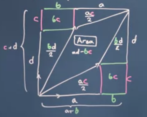
Definition of the determinant (for a $2\times 2$ matrix)
The determinant of the matrix
$$A = \left( \begin{array}{cc} a & b\\ c & d \end{array} \right) \in \mathbb{R}^{2 \times 2}$$is denoted by $\det(A)$ and can be calculated as $a\cdot d - b \cdot c$.
The absolut value of the determinant and the area of the parallelipiped
Observe that the above determinant is exactly the area of the parallelogram spanned by the vectors
$\left(
\begin{array}{c}
a\\
c
\end{array}
\right)$ and $\left(
\begin{array}{c}
b\\
d
\end{array}
\right)$
if the second vector is situated into a positive direction w.r.t. the first one. Otherwise the determinant is has a negative sign, but its absolute value is still equal to the area.
The exact definition of the determinant is for higher dimensional matrices is overwhelming. For our calculations it is enough to know that the absolute value of is always equal to the volume of the parallelipiped spanned by the column vectors of the matrix.
Characterisation of linear dependence with the help of the determininant A reformulation of the definition of linear dependency says that the vectors $v_1, v_2, \ldots, v_n \in mathbb{R}^n$ are linearly dependent if they do not span the whole space $\mathbb{R}^n$. This situation is characterised by the fact the parallelipiped spanned by these vectors is degenerate and its volume is 0.
Let us denote the matrix containing on its column the vectors $v_1, v_2, \ldots, v_n$ by $V$. By the relation between the volume of the parallelipiped mentioned before and $\det(V)$, we can claim the following
"The vectors $v_1, v_2, \ldots, v_n \in \mathbb{R}^n$ are linearly dependent is and only if $\det(V) = 0$, where the matrix containing on its column the vectors $v_1, v_2, \ldots, v_n$."
Furthermore, equivalently
"The vectors $v_1, v_2, \ldots, v_n \in \mathbb{R}^n$ are linearly independent is and only if $\det(V) \neq 0$, where the matrix containing on its column the vectors $v_1, v_2, \ldots, v_n$."
Exercise
Let us consider a $2 \times 2$ dimensional real matrix with non-zero determinant given as $A = \left( \begin{array}{cc} a & b\\ c & d \end{array} \right)$
Show that
$$A^{-1} = \frac{1}{ad-bc}\left( \begin{array}{cc} d & -b\\ -c & a \end{array} \right)$$Exercise
The reference vectors (basis vectors) of our friend used to express vectors $\in \mathbb{R}^2$ are different from the canonical ones: $u = \left( \begin{array}{c} 2\\ 3 \end{array} \right)$, $v = \left(\begin{array}{c} 3\\ 4 \end{array} \right)$. He would like to perform a rotation by $60^°$ in his coordinate system.
We know that in the canonical coordinate system a rotation can be achieved by mutiplying the vector from left by the rotation matrix
Can you give a formula that would perform the rotation in the basis of our friend?
Answer
We know the transformation matrix describing the phenomenon in the canonical basis:
$$R_{60^°} = \left( \begin{array}{cc} \cos(60^°) & -\sin(60^°)\\ \sin(60^°) & \cos(60^°) \end{array} \right) = \left( \begin{array}{cc} \frac{1}{2} & -\frac{\sqrt{3}}{2}\\ \frac{\sqrt{3}}{2} & \frac{1}{2} \end{array} \right)$$We need to rewrite it in the basis determined by the vectors $u$ and $v$. Namely we would like to provide the matrix transformation that maps a vector given in the basis of the friend into the image vector (which is just the rotation by $60^°$ of the starting vector) expressed also in the basis of the friend.
The recipe is the following:
- We start with a vector $x$ expressed in the basis of the friend as $\left(\begin{array}{c} x_1\\ x_2 \end{array}\right)$, i.e. $[x]_{\{u,v\}} = \left(\begin{array}{c} x_1\\ x_2 \end{array}\right)$.
- We express its coordinates w.r.t. the canonical basis by the change of basis formula
- We apply the transformation matrix, which describes the rotation in the canonical basis. The coordinates of the rotated vector in the canonical basis will be
- Lastly we express the rotated vector in the basis of the friend. As the transformation from the coordinates of the friend to the canonical ones is described by the matrix $\left(\begin{array}{cc} 2 & 3\\ 3 & 4 \end{array}\right)$, the inverse mapping transforming the canonical coordinates of a vector to the coordinates w.r.t. the basis of the friend is described by the inverse of this mapping, that is the inverse of the matrix $\left(\begin{array}{cc} 2 & 3\\ 3 & 4 \end{array}\right)$. Thus the result vector expressed in the coordinates of the friend is
Finally the mapping
$$\left(\begin{array}{c} x_1\\ x_2 \end{array}\right) \mapsto \left(\begin{array}{cc} 2 & 3\\ 3 & 4 \end{array}\right)^{-1} \cdot \left( \begin{array}{cc} \frac{1}{2} & -\frac{\sqrt{3}}{2}\\ \frac{\sqrt{3}}{2} & \frac{1}{2} \end{array} \right) \cdot \left(\begin{array}{cc} 2 & 3\\ 3 & 4 \end{array}\right) \cdot \left(\begin{array}{c} x_1\\ x_2 \end{array}\right)$$is the linear mapping given by the matrix
$$\left(\begin{array}{cc} 2 & 3\\ 3 & 4 \end{array}\right)^{-1} \cdot \left( \begin{array}{cc} \frac{1}{2} & -\frac{\sqrt{3}}{2}\\ \frac{\sqrt{3}}{2} & \frac{1}{2} \end{array} \right) \cdot \left(\begin{array}{cc} 2 & 3\\ 3 & 4 \end{array}\right)$$In general if $C$ is the change of basis vector describing the tranformation from the coordinates given in the basis $\{c_{\cdot, 1}, \ldots, c_{\cdot, m}\}$ to the canonical coordinates, i.e.
$$C\cdot [x]_{\{c_{\cdot, 1}, \ldots, c_{\cdot, m}\}} = [x]_{\{e_{\cdot, 1}, \ldots, e_{\cdot, m}\}}$$and $T$ is the matrix which describes the desired transformation in the canonical basis, then the same transformation w.r.t. the basis $\{c_{\cdot, 1}, \ldots, c_{\cdot, m}\}$ is described by the matrix
$$C^{-1} \cdot T \cdot C.$$2.3.6. Orthogonal matrices and Gram-Schmidt orthogonalisation
Definition of orthogonal matrices A square matrix $Q \in \mathbb{R}^{n\times n}$ is said to be orthogonal if
$$Q \cdot Q^T = Q^T \cdot Q= I_n.$$This is equvalent to the fact that the columns of the matrix $Q$ form an orthogonal basis of $\mathbb{R}^n$.
Furthermore, this is also equivalent to the fact that the rows of the matrix $Q$ form an orthogonal basis of $\mathbb{R}^n$.
Remark
Orthogonal matrices have the nice property that their transposed is their inverse. That's why we like to work with them more than with other matrices. Consequently we prefer also the orthonormal basis to the other ones.
Definition of orthogonal basis and orthonormal basis
A basis $\{b_1, b_2, \ldots, b_n\}$ of a vectors space $V$ is called orthogonal if the basis vectors are pairwise orthogonal to each other, i.e. $\langle b_i, \rangle b_j = 0$ for any $i \neq j$.
If in addition each basis vector has norm 1, then the basis is called orthonormal.
How can we transform a basis into an orthonormal basis?
The video shows us exactly such an orthogonalisation.
Question
What do you observe? Identify the steps that are performed.
IFrame("https://www.geogebra.org/classic/cyvs2mur", 800, 600)
The process you could observe in the video is called Gram-Schmidt orthogonalisation. In the forthcoming we explain the steps in detail.
Gram-Schmidt orthogonalisation
Let's see how can we transform a basis to an orthonormal basis in $\mathbb{R}^n$.
Let us consider a vector space $V$ with a basis given by the vectors $x_1, x_2, \ldots x_n$. We will modify the basis iteratively, changing at each step just one of the elements of the basis.
Step 1: We change the basis element $x_1$ by normalising it. The new basis is now compound of
$$u_1 = \frac{x_1}{||x_1||}, x_2, \ldots, x_n$$
Step 2: We modify the basis element $x_2$. We would like that this new basis element $v_2$ is orthogonal to the first one and ${\rm span}(\{u_1, v_2\}) = {\rm span}(\{u_1, x_2\})$. From this condition we get that $v_2$ should be the projection of $x_2$ to the orthogonal complement of $\{x_1\}$ or equivalently $v_2 = x_2 - \pi_{u_1}{x_2}$
The new basis is now compound of
$$u_1 = \frac{x_1}{||x_1||}, v_2 = x_2 - \pi_{u_1}{x_2}, x_3 \ldots, x_n$$
Step 3: We normalise $v_2$. The new basis is now compound of
$$u_1, u_2 = \frac{v_2}{||v_2||}, x_3 \ldots, x_n$$
Step 4: We modify the basis element $x_3$. We would like that this new basis element $v_3$ is orthogonal to the previous two ones $u_1$ and $u_2$ and ${\rm span}(\{u_1, u_2, v_3\}) = {\rm span}(\{u_1, u_2, x_3\})$. From this condition we get that
The new basis is compound of
$$u_1, u_2, v_3 = x_3 - \pi_{u_1}(x_3) - \pi_{u_2}(x_3), x_4 \ldots, x_n$$
Step 5: We normalise $v_3$. The new basis is
$$u_1, u_2, u_3 = \frac{v_3}{||v_3||}, x_4 \ldots, x_n$$
We continue this process so until all the basis vectors are exchanged.
Remark
Observe that the above transformations are all such linear transformation that preserves the linear independence of the vectors of the basis in each step. This is crutial to make sure that we end up also with a basis.
Remark
If we start to orthogonalise a set of vectors about which we don't know whether they are linearly independent, then during the iterative transformation it might happen that some of the new vectors will be $\mathbf{0}$. We realise this latest when we would like to normalise thsi vector and we cannot divide by its norm. If we encounter this situation, this means that the original vectors that we started with were not linearly independent.
Exercise
Determine the transformation matrix, which is describing the reflection w.r.t. the vectors $\left( \begin{array}{c} 1\\ 0\\ 2 \end{array} \right)$ and $\left( \begin{array}{c} 0\\ 2\\ 2 \end{array} \right)$.
2.3.7. Eigenvectors, eigenvalues
Eigenvectors of a matrix $A$ are the vectors, which are just scaled by a factor when appliying the matrix transformation on them. The eigenvalues are the corresponding factors.
Use this informal definition of eigenvalues and eigenvectors to answer the following exercise.
Exercise
Associate the following transformations in $\mathbb{R}^2$ to the number of eigenvectors that they have:
- Rotation in $\mathbb{R}^2$
- Rotation in $\mathbb{R}^3$
- Scaling along one axis
- Scaling along 2 axis
- Multiplication by the identity matrix
Number of eigenvectors:
a. every vector is an eigenvector
b. the transformation has exactly 2 eigenvectors
c. the transformation has exactly one eigenvectors
d. the transformation can have none or two eigenvectors
It can be handy to use the below tool for visualising the eigenvectors.
IFrame("https://www.geogebra.org/classic/ncp2peap", 1000, 600)
Formal definition of eigenvectors and eigenvalues
Let us consider a square matrix $A \in \mathbb{R}^{n \times n}$. We say that the non-zero vector $v \in \mathbb{R}^n$ is an eigenvector of $A$ and $\lambda$ is the associated eigenvalue if
$$A \cdot v = \lambda v.$$Remark
As a consequence of the above definition an eigenvalue $\lambda$ should satisfy
or equivalently
As the vector $(A - \lambda I_n) \cdot v$ is a linear combination of the columns of $A - \lambda I_n$ with not all zero coefficients, the above equation tells the columns of the matrix $A - \lambda I_n$ are linearly dependent. Using the characterisation of linear dependency with the help of determinants, this is equivalent to the fact that
$$\det(A-\lambda I_n) = 0$$For our setting the expression on the left hand side will be a polynomial of order $n$ in $\lambda$, which is called the characteristic polynomial of $A$. The solutions of the characteristic polinomial will be our eigenvalues.
After determining an eigenvalue $\lambda^*$, we can calculate the corresponding eigenvector(s), by solving the equation
$$(A - \lambda^* I_n) \cdot v = \mathbf{0}$$3. Homework
Read through the linear algebra part of this course and summarise the elevant formulas a cheat sheet.