![]()
![]()
3. Calculus
Agenda
- differentiation of univariate functions
- rules of differentiation
- differentiation of multivariate functions (the Jacobian, the Hessian)
- chain rule for univariate and multivariate functions
- the Taylor approximation
- the Newton-Raphson method
- gradient descent method
- backpropagation
3.1. Motivation
Find the optimal value of the model parameters of a neuronal network.
3.2. Functions
A function $f:A \to B$ associates to each element of the set $A$ an element of the set $B$.
For our future context $A = \mathbb{R}^n$ and $B = \mathbb{R}^m$ for some natural numbers $n$ and $m$.
3.2.1. Differentiation of a function (univariate case)
For a function $f:\mathbb{R} \to \mathbb{R}$ we would like characterise its local linear behavior. Therefore we take two points $x$ and $x+\Delta x$ and their corresponding values $f(x)$ and $f(x+\Delta x)$. We are going to connect these points by a line and we will calculate the gradient of this line
$$m = \frac{\Delta f}{\Delta x} = \frac{f(x+\Delta x)-f(x)}{(x+\Delta x) - x} = \frac{f(x+\Delta x)-f(x)}{\Delta x}$$Now we are going to take smaller and smaller values for the increment $\Delta x$. We define the derivative of $f$ in point $x$ as the value of the above quotient when $\Delta x$ is getting infinitesimally small.
The mathematically exact formula for the derivative is
$$f'(x) = \lim\limits_{\Delta x \to 0} \frac{f(x+\Delta x)-f(x)}{\Delta x}$$from IPython.display import IFrame
IFrame("https://www.geogebra.org/classic/enyhcvgw", 1100, 900)
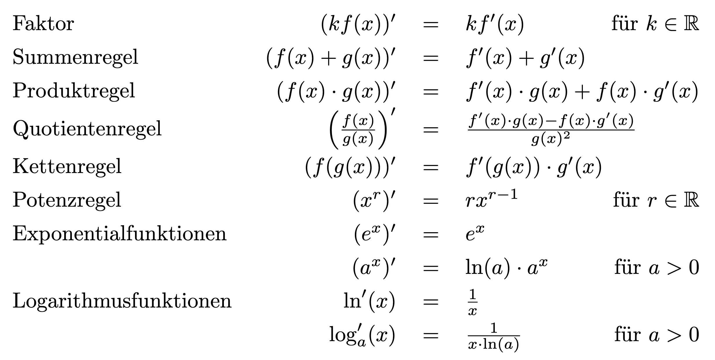
3.2.2. Differentiation rules
3.2.3. Differentiation of a function (multivariate case)
When the function $f:\mathbb{R}^n \to \mathbb{R}$ depends on more variables $x_1, x_2, \ldots, x_n$ and it is nice enough, we can calculate its partial derivatives w.r.t. each variable. The partial derivative of the function $f$ in a point $x^* =(x_1^*, x_2*, \ldots, x_n^*)$ w.r.t. the variable $x_1$ can be calculated by fixing the values of the other parameters to be equal to $x_2^*, \ldots, x_n^*$ and derivating the so resulting function by its only parameter $x_1$.
To describe the formula in a mathematical exact way let us consider the function $g: \mathbb{R} \to \mathbb{R}$ defined by the formula
$$g(x_1) = f(x_1, x_2^*, \ldots, x_n^*)$$Then the partial derivative of $f$ w.r.t. $x_1$ is denoted by $\frac{\partial f}{\partial x_1}$ and is equal to the derivative of $g$ in the point $x_1*$, that is
$$\frac{\partial f}{\partial x_1}(x_1^*,, x_2^*, \ldots, x_n^*) = g'(x_1)$$Alternatively we can use for this partial derivative also other notations like the shorter
$$\frac{\partial f}{\partial x_1}(x^*) \quad \mbox{or} \quad \partial_{x_1} f(x*)$$When it clear that we are performing our calculations in the point $x^*$ and there is no source for confusion, we can omit $x^*$ also and work just with
$$\frac{\partial f}{\partial x_1} \quad \mbox{or} \quad \partial_{x_1} f$$We can proceed similarly in the case of the other variables to calculate all partial derivatives
$$\frac{\partial f}{\partial x_2}(x^*), \quad \frac{\partial f}{\partial x_3}(x^*), \quad \ldots \quad, \frac{\partial f}{\partial x_n}(x^*)$$The row vector of all partial derivatives is called the gradient of the function or the Jacobian of it, that is $$ \nabla f = \left( \frac{\partial f}{\partial x_1}, \frac{\partial f}{\partial x_2}, \ldots \frac{\partial f}{\partial x_n}\right)$$
The gradient or Jacobian of the function $f$ has the following two properties, which are crutial for our forthcoming applications:
- in a fixed point $x* =(x_1^*, x_2*, \ldots, x_n*)$ the gradient/ Jacobian $\nabla f$ points up the hill along the steepest direction
- its length is proportional to the steepness.
Further generalisation
For a function $f: \mathbb{R}^n \to \mathbb{R}^m$ having also a multivariate output, we can take each output and calculate its partial derivatives w.r.t. each input variable $x_1, x_2, \ldots, x_n$. For the first output we will have $n$ partial derivatives,i.e.
And for each output the same will happen. We will organise these partial derivatives in a matrix in such a way that in the $i$th row the derivatives of $f_i$ will be enlisted, and at the intersection of $i$th row and $j$th column the derivative
$$\frac{\partial f_i}{\partial x_j}$$will be stored.
This way we obtain the matrix
$$\nabla f = \left( \begin{array}{cccc} \frac{\partial f_1}{\partial x_1} & \frac{\partial f_1}{\partial x_2} & \cdots & \frac{\partial f_1}{\partial x_n}\\ \frac{\partial f_2}{\partial x_1} & \frac{\partial f_2}{\partial x_2} & \cdots & \frac{\partial f_2}{\partial x_n}\\ \vdots & \vdots & \ddots & \vdots\\ \frac{\partial f_m}{\partial x_1} & \frac{\partial f_m}{\partial x_2} & \cdots & \frac{\partial f_m}{\partial x_n} \end{array} \right)$$This matrix is called the Jacobian of the function $f$.
3.2.4. Higher order differentials (uni- and multivariate case)
For a function $f: \mathbb{R}\to \mathbb{R}$ we can calculate its derivative in each point, this means that the derivative $f'$ of the function is again a function mapping each point $x \in \mathbb{R}$ to the derivative $f'(x)$.
Now we could differentiate again each the first order derivative $f'$ and as such we get to the second order derivative, i.e.
$$f''(x) = \lim\limits_{\Delta x \to 0}\frac{f'(x+\Delta x) - f'(x)}{\Delta x}$$The second order derivative can be again derivated and this way we obtain the $3$rd order derivative of a function.
Multivariate case
We extend the notion of second order derivative to a function $f: \mathbb{R}^n \to \mathbb{R}$.
Consider as starting point the Jacobian of the function (which corresponds to the derivative from the univariate case). Let us calculate all partial derivatives of the first order partial derivatives from
$$\nabla f = \left( \frac{\partial f}{\partial x_1}, \frac{\partial f}{\partial x_2}, \ldots \frac{\partial f}{\partial x_n}\right),$$and organize them in the following way in a matrix
$$\nabla^2 f = \left( \begin{array}{cccc} \frac{\partial^2 f}{\partial x_1\partial x_1} & \frac{\partial^2 f}{\partial x_1\partial x_2} & \cdots & \frac{\partial^2 f}{\partial x_1\partial x_n} \\ \frac{\partial^2 f}{\partial x_2\partial x_1} & \frac{\partial^2 f}{\partial x_2\partial x_2} & \cdots & \frac{\partial^2 f}{\partial x_2\partial x_n} \\ \vdots & \vdots & \ddots & \vdots\\ \frac{\partial^2 f}{\partial x_n\partial x_1} & \frac{\partial^2 f}{\partial x_n\partial x_2} & \cdots & \frac{\partial^2 f}{\partial x_n\partial x_n} \end{array} \right)$$then the resulting matrix is called the Hessian matrix.
The value of the Hessian matrix can be used
- to derive better local approximation for a function than the linear one,
- to find out whether a critical point is a minimum or maximim point or saddle point (exacly as the second order derivative helps us determine whether a critical point is an extreme point of the function).
IFrame("https://www.geogebra.org/classic/kc2umqak", 1000, 800)
Taylor polynomial of order $n$
The Taylor polynomial of order $n$ of a smooth enough function $f: \mathbb{R} \to \mathbb{R}$ around the point $x = x_0$ is given by the following formula
$$p(x) = \frac{f(x_0)}{0!} + \frac{f'(x_0)}{1!}(x-x_0) + \frac{f''(x_0)}{2!} + \cdot + \frac{f^{(n)}(x_0)}{n!} (x-x_0)^n$$Where $0! = 0$ by convention.
If the function is nice enough, then the approximation error:
$f(x) - p(x)$ is of magnitude $(x-x_0)^n$.
Remark
The above polinomial has the property that the function value and the first $n$ derivatives of the original function $f$ and the polynomial $p$ are exactly the same in the point $x=x_0$. This polynomial is uniquely defined.
The Taylor approximation of a multivariate function For a function $f: \mathbb{R}^n \to \mathbb{R}$ the Taylor approximation of order 1 is
$$l(x) = \frac{f(x_0)}{0!} + \frac{\nabla f(x_0)}{1!}\cdot (x-x_0),$$where $\nabla f(x_0)$ denotes the Jacobian of the function in point $x_0$ and this row vector is multiplied by the column vector $x-x_0$ in the above formula.
For a function $f: \mathbb{R}^n \to \mathbb{R}$ the Taylor approximation of order 2 is
$$q(x) = \frac{f(x_0)}{0!} + \frac{1}{1!}\nabla f(x_0)\cdot (x-x_0) + \frac{1}{2} (x-x_0)^T \cdot \nabla^2 f(x_0) \cdot (x-x_0),$$where $\nabla^2 f(x_0)$ denotes the Hessian of the function in point $x_0$ and this matrix is multiplied from left by the row vector $(x-x_0)^T$ nd from the right by the column vector $x-x_0$ in the above formula.
3.3.2. The Newton-Raphson method
The Newton-Raphson method is used to find the approximate a root of a function.
Observe how does it work and identify the steps of the method.
IFrame("https://www.geogebra.org/classic/mm9xvyxr", 800, 600)
The Newton-Raphson method is an iterative method.
We cosider a function $f:\mathbb{R} \to \mathbb{R}$
The purpose of this method is to approximate roots of the function, i.e. such $x$ values for which $f(x) = 0$.
Let us assume that we know the value of the function in a point $x_0$, i.e we know $f(x_0)$. We approximate the behaviour of the function by the tangent line
$$f(x) \simeq l(x) = f(x_0) + f'(x_0)\cdot (x-x_0)$$and we solve the equation
$$l(x) = 0$$The solution of this will be denoted by $x_1$ and by solving the above linear equation we obtain that
$$x_1 = x_0 - \frac{f(x_0)}{f'(x_0)}$$$x_1$ is our second approximation for a root of $f$.
If we continue the process now by constructing the tangent line in $x_1$ and defining the next point as an intersection of the tangent with the $x$-axis, then
$$x_2 = x_1 - \frac{f(x_0)}{f'(x_0)}$$will be our third approximation for the root.
If the function is nice enough, then this method converges to a root of the function.
3.3.3. Gradient descent method
The gradient descent method is similar to the Newton-Raphson one in the sense that we perform an iterative step in the steepest direction. The difference is that the goal of this process is to minimise a cost function $C: \mathbb{R} \to \mathbb{R}$ (or $C: \mathbb{R} \to \mathbb{R}$ in the multivariate case). We update the gradient in every iterative step and we move along the steepest gradient downwards, i.e.
$$x_{n+1} = x_{n} - \lambda \nabla f(x_n).$$IFrame("https://www.geogebra.org/classic/xfa7y3wc", 800, 600)
3.3.4. Backpropagation
See the blackboard