The IS-LM model

EC 235 | Fall 2023

Materials

Required readings:

Blanchard, ch. 5.

Prologue

The previous two chapters introduced the goods and financial markets, respectively.

In the first, we explored the determinants of aggregate demand (Z), and how equilibrium can be reached when production (Y) is met by aggregate expenditures.

In the second, we saw that the interest rate plays a key role in the demand for and supply of money, and how equilibrium may be reached through monetary policy.

However, just looking at these two markets on their own is not sufficient to fully understand the macroeconomy.

Prologue

Now we turn to the IS-LM model, which combines the goods and money markets for a more comprehensive macroeconomic analysis.

The IS relation

Recall aggregate demand in a closed economy:

\[ Z = C + \bar{I} + G \]

And we assumed that C is a function of disposable income (Y_D), and I and G were exogenously determined.

Moving on, we will abandon the assumption that aggregate investment (I) is given.

The IS relation

Aggregate investment is in fact far from constant and depends primarily on two factors:

The level of sales;
The interest rate.

First, firms facing increases in sales will need to invest further in order to increase production.

Second, firms almost never have the entirety of funds to finance themselves to make such investments. Thus, they need to borrow from the money market.

The IS relation

Given this motivation, we may write the investment function as:

\[ I = I(Y, i) \hspace{1cm} \dfrac{\partial I}{\partial Y} > 0 \ \ ; \ \ \dfrac{\partial I}{\partial i} < 0 \]

In words, an increase in output (Y) increases investment; and an increase in the interest rate (i) decreases investment.

The IS relation

Now we can rewrite the aggregate demand function Z as:

\[ Z = C(Y_D) + I(Y,i) + G \]

And we know that equilibrium in the goods market (Y = Z) also implies that investment equals savings:

\[ I = S \]

The IS relation

The name IS comes from Investment-Saving.

Thus, let us use this last equilibrium condition to derive the IS curve.

Intuitively, we would like to find all combinations of the interest rate (i) and output (Y) that bring equilibrium to the goods market.

The IS relation

What factors will affect the slope of the the IS curve?

What factors will shift the IS curve?

The LM relation

Now, we turn to the financial market.

We all know that the demand for money (M^D) depends on income (Y) and on the interest rate (i):

\[ M^D = PY \cdot L(i) \]

And equilibrium in the money market is reached when the supply of money (M^S) is met by money demand:

\[ M^D = M^S \]

The LM relation

The name LM comes from Liquidity-Money.

Thus, let us use this last equilibrium condition to derive the LM curve.

Intuitively, we would like to find all combinations of the interest rate (i) and output (Y) that bring equilibrium to the money market.

The LM relation

What factors will affect the slope of the the LM curve?

What factors will shift the LM curve?

The IS-LM model

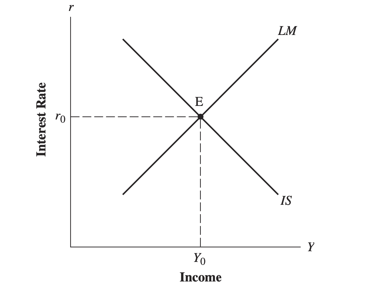
The IS-LM model

The upward-sloping LM schedule shows the points of equilibrium for the money market.

The downward- sloping IS schedule shows the points of equilibrium for the goods market.

The point of intersection between the two schedules is the (only) point of general equilibrium for the two markets.

The IS-LM model

Let us now explore this further with an example.