The goods market
EC 235 | Fall 2023
Materials
Required readings:
- Blanchard, ch. 3.
The composition of GDP
After reviewing some of the most important macroeconomic variables—output, (un)employment, and inflation—, it is time to start diving into the actual name of this course:
- Macroeconomic Theory!
And we will start this process by looking at the composition of aggregate output (GDP).
Never forget:
\[ \text{GDP} = C + I + G + (X - IM) \]
The composition of GDP
Again:
\[ \text{GDP} = C + I + G + (X - IM) \]
where:
- C: aggregate consumption;
- I: aggregate investment;
- G: government expenditures;
- X: exports;
- IM: imports.
The composition of GDP
Important remarks:
Investment (I) in the macro sense is NOT the same as purchasing financial assets!
I also includes changes in inventories;
Government spending (G) does NOT include transfer payments (e.g., Medicare and Social Security);
The difference between exports and imports (X - IM) is also known as the trade balance.
The composition of GDP
The demand for goods
Defining the whole economy’s demand for goods and services (goods, for short) as Z, we can write the following identity:
\[ Z \equiv C + I + G + (X - IM) \]
For simplicity’s sake, our analysis will start off by assuming a closed economy (i.e., a country that does not do business with the rest of the world):
\[ Z \equiv C + I + G \]
Now, we can start modeling the (macro)economy.
The demand for goods
Now, we can start modeling the (macro)economy.
But what perspective are we adopting to model the macroeconomy?
The demand for goods
The demand for goods
Starting off with aggregate consumption (C), it is a positive function of disposable income (YD):
\[ C = C(Y_D) \]
where
\[ \hspace{1cm} \dfrac{\partial{C}}{\partial{Y_D}} > 0 \]
Here, C(YD) denotes a behavioral equation representing the aggregate consumption function of this economy.
The demand for goods
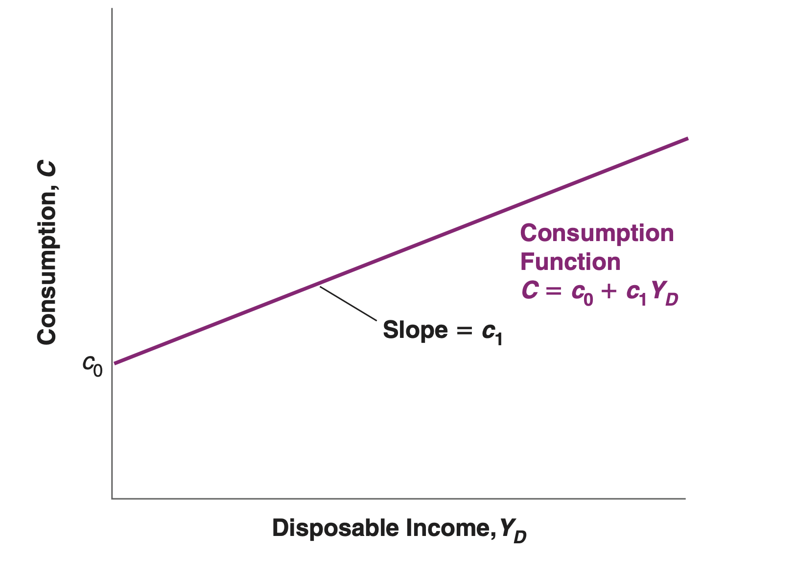
The simplest way to define the functional form of the consumption function is through a linear representation like
\[ C = c_0 + c_1Y_D \]
In words:
Aggregate consumption is a linear function of disposable income;
c0 represents autonomous consumption (i.e., independent of income);
c1 is the economy’s (marginal) propensity to consume.
- What does c1 represent?
The demand for goods
The demand for goods
Since YD = Y - T, we can rewrite the consumption function as
\[ C = c_0 + c_1\underbrace{(Y - T)}_{\text{disposable income}} \]
What are the effects of:
Aggregate income (Y) on consumption?
Taxes (T) on consumption?
The demand for goods
Moving on to aggregate investment, I, we will assume (for the time being) that it is given exogenously:
\[ I = \bar{I} \]
We will relax this assumption later on.
The demand for goods
Finally, government spending (G) denotes one component of fiscal policy.
The other are Net Taxes (T).
We will also assume that public spending and taxes are exogenous.
The demand for goods
Now we are ready to write a more detailed equation for aggregate demand:
\[ Z \equiv c_0 + c_1(Y - T) + \bar{I} + G \]
Equilibrium output
Equilibrium output
Equilibrium in the goods market requires that production Y be equal to the demand for goods Z:
\[ Y = Z \]
Let us explore this scenario in three ways:
- Algebraically;
- Graphically;
- Verbally.
Investment = Saving
Investment = Saving
An alternative way of looking at the equality between production and demand is to focus on investment (I) and saving (S).
Private saving (S) (i.e., consumers’ saving) is the remainder of their disposable income after consumption:
\[ S \equiv Y_D - C \]
Or, equivalently,
\[ S \equiv Y - T - C \]
Investment = Saving
The previous identity concerns the private sector.
We can include the public sector by recalling aggregate output (Y):
\[ Y = C + I + G \]
Subtract taxes (T) and consumption (C) on both sides:
\[ Y - C - T = I + G - T \]
Investment = Saving
\[ \underbrace{Y - C - T}_S = I + G - T \]
\[ S = I + G - T \]
\[ I = S + (T - G) \]
The left-hand side is the sum of private and public saving.
Investment = Saving
\[ I = S + (T - G) \]
This relation states that equilibrium in the goods market requires that aggregate investment equals saving—the sum of private and public saving.
In other words, what firms want to invest must be equal to what people and the government want to save.
Investment = Saving
Starting from:
\[ S_p = Y - T - C \]
Using the definition of aggregate consumption (C), find an expression for aggregate saving (S) containing autonomous consumption (c0) and the marginal propensity to save (1 - c1).
EC 235 - Prof. Santetti