Welcome! 👋

The practical component of the Statistical Modeling & Causal Inference course relies largely on R programming. Today will center around some of the necessary skills to perform the assignments for this course.

This week’s primer will be divided in two parts. Today, we will focus on three aspects:

First, we will speak about the R and RStudio infrastructure setup.
Second, we will remind you of the most important data structures in R and we will practice some basic commands to get you up to speed with working in R.
Third, we will discuss some best practices in R.

But first things first: Have you all successfully installed R and RStudio? Otherwise, install R first, then install RStudio - or think about updating R, RStudio, and your installed packages.

R and RStudio: Basics

The RStudio interface

RStudio is an integrated development environment (IDE) for R. Think of RStudio as a front that allows us to interact, compile, and render R code in a more instinctive way. The following image shows what the standard RStudio interface looks like:

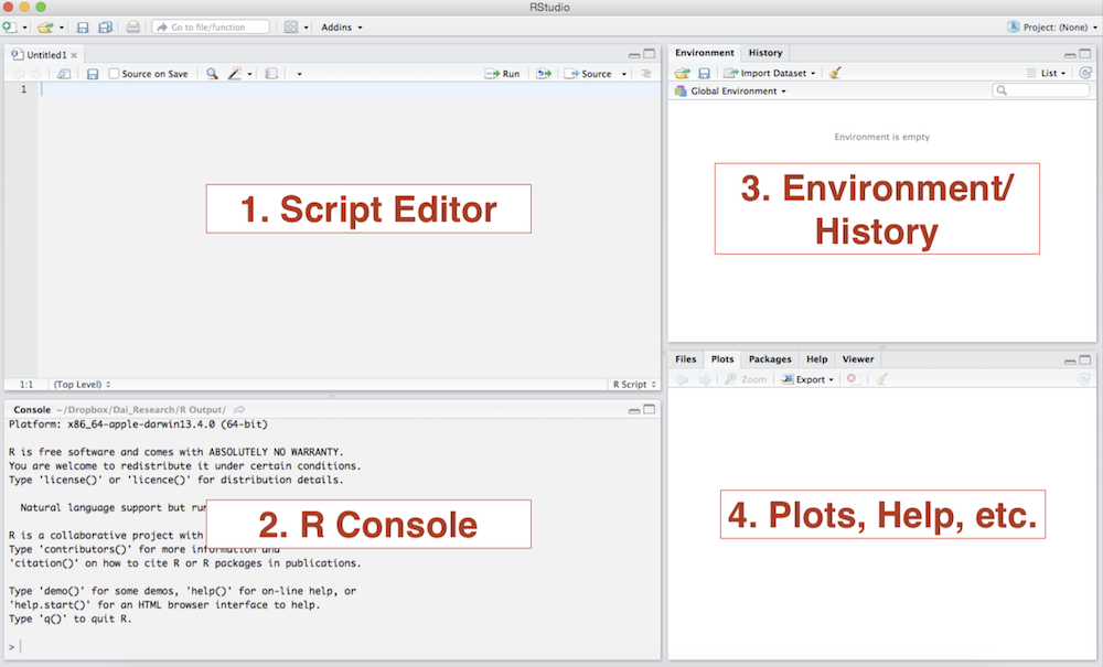
RStudio Interface

Console: The console provides a means to interact directly with R. You can type some code at the console and when you press ENTER, R will run that code. Depending on what you type, you may see some output in the console or if you make a mistake, you may get a warning or an error message.
Script editor: You will utilize the script editor to complete your assignments. The script editor will be the space where files will be displayed. For example, once you download and open the bi-weekly assignment .Rmd template, it will appear here. The editor is a where you should place code you care about, since the code from the console cannot be saved into a script.
Environment: This area holds the abstractions you have created with your code. If you run myresult <- 5+3+2, the myresult object will appear there.
Plots and files: This area will be where graphic output will be generated. Additionally, if you write a question mark before any function, (i.e. ?mean) the online documentation will be displayed here.

Getting Help 🔎

The key to learning R is: Google! We can give you an overview over basic R functions, but to really learn R you will have to actively use it yourself, trouble shoot, ask questions, and google! Help pages such as http://stackoverflow.com offer a rich archive of questions and answers by the R community. For example, if you google “recode data in r” you will find a variety of useful websites explaining how to do this on the first page of the search results. Also, don’t be surprised if you find a variety of different ways to execute the same task.

RStudio also has a useful help menu. In addition, you can get information on any function or integrated data set in R through the console, for example:

?plot

In addition, there are a lot of free R comprehensive guides, such as Quick-R at http://www.statmethods.net or the R cookbook at http://www.cookbook-r.com.

Executing a line of code

To execute a single line of code. In RStudio, with the curser in the line you want R to execute,

Press command + return (on macOS) or Crtl + Enter (on Windows).

To execute multiple lines of code at once, highlight the respective portion of the code and then run it using the operations above.

Arithmetic in `R` 👨‍🏫

You can use R as a calculator!

	Operator	Example
Addition	`+`	`2+4`
Subtraction	`-`	`2-4`
Multiplication	`*`	`2*4`
Division	`/`	`4/2`
Exponentiation	`^`	`2^4`
Square Root	`sqrt()`	`sqrt(144)`
Absolute Value	`abs()`	`abs(-4)`

4*9

## [1] 36

sqrt(144)

## [1] 12

Logical operators 🤔

	Operator
Less than	`<`
Less than or equal to	`<=`
Greater than	`>`
Greater than or equal to	`>=`
Exactly equal to	`==`
Not equal to	`!=`
Not `x`	`!x`
`x` or `y`	`x \| y`
`x` and `y`	`x & y`

Logical operators are incredibly helpful for any type of exploratory analysis, data cleaning and/or visualization task.

4 > 2

## [1] TRUE

4 <= 2

## [1] FALSE

Objects in R

R stores information as an object. You can name objects whatever you like. Just remember to not use names that are reserved for build-in functions or functions in the packages you use, such as sum, mean, or abs. Most of the time, R will let you use these as names, but it leads to confusion in your code.

Assigning values to objects

A few things to remember

Do not use special characters such as $ or %. Common symbols that are used in variable names include . or _.
Remember that R is case sensitive.
To assign values to objects, we use the assignment operator <-. Sometimes you will also see = as the assignment operator. This is a matter of preference and subject to debate among R programmers. Personally, I use <- to assign values to objects and = within functions.
The # symbol is used for commenting and demarcation. Any code following # will not be executed.

Below, R stores the result of the calculation in an object named result. We can access the value by referring to the object name.

result <- 5/3
result

## [1] 1.666667

If we assign a different value to the object, the value of the object will be changed.

result <- 5-3
result

## [1] 2

Data Types in R

There are four main variable types you should be familiar with:

Numerical: Any number. Integer is a numerical variable without any decimals.
Character: This is what Stata (and other programming languages such as Python) calls a string. We typically store any alphanumeric data that is not ordered as a character vector.
Logical: A collection of TRUE and FALSE values.
Factor: Think about it as an ordinal variable, i.e. an ordered categorical variable.

Data Structures in R

R has many data structures, the most important ones for now are:

Vectors
Lists
Matrices
Data frames
Factors

Here is a short overview with a few related operations that you can apply to the different structures.

Vectors

my_vector <- c(1, 2, 3)
my_character_vector <- c("Welcome", "everyone")
length(my_vector)

## [1] 3

str(my_character_vector)

##  chr [1:2] "Welcome" "everyone"

Matrices

my_matrix <- matrix(nrow=3, ncol=3)
dim(my_matrix)

## [1] 3 3

Lists

my_list <- list(1, "a", TRUE)
my_list[2]

## [[1]]
## [1] "a"

my_list[[2]]

## [1] "a"

Data Frames

my_df <- data.frame(id = letters[1:10], x = 1:10, y = 11:20)

Some useful operations to learn something about a data frame - more on this in a moment!

head(my_df)
tail(my_df)
dim(my_df)
nrow(my_df)
ncol(my_df)
str(my_df)
names(my_df)

Factors

# direct creation of factors
my_factor <- factor(c("single","single","married","married","single"))

# turning vectors into factors
my_vector <- c("single","single","married","married","single")
my_factor <- as.factor(my_vector)

levels(my_factor)

## [1] "married" "single"

If you are thrilled by object classes in R by now, here is more.

Vectors ⬇️

Let’s first focus on vectors as building blocks of most data structures you’ll be working with.

A vector is one of the simplest type of data you can work with in R. “A vector or a one-dimensional array simply represents a collection of information stored in a specific order” (Imai 2017: 14). It is essentially a list of data of a single type (e.g. numerical, character, or logical).

To create a vector, we use the function c() (concatenate) to combine separate data points. The general format for creating a vector in R is as follows: name_of_vector <- c("what you want to put into the vector")

Suppose, we have data on the population in millions for the five most populous countries in 2016. The data come from the World Bank.

pop1 <- c(1379, 1324, 323, 261, 208)
pop1

## [1] 1379 1324  323  261  208

We can use the function c() to combine two vectors. Suppose we had data on 5 additional countries.

pop2 <- c(194, 187, 161, 142, 127)
pop <- c(pop1, pop2)
pop

##  [1] 1379 1324  323  261  208  194  187  161  142  127

First, lets check which variable type our population data were stored in. The output below tells us that the object pop is of class numeric, and has the dimensions [1:10], that is 10 elements in one dimension.

str(pop)

##  num [1:10] 1379 1324 323 261 208 ...

Suppose, we wanted to add information on the country names. We can enter these data in character format. To save time, we will only do this for the five most populous countries.

cname <- c("CHN", "IND", "USA", "IDN", "BRA")
str(cname)

##  chr [1:5] "CHN" "IND" "USA" "IDN" "BRA"

Now, lets code a logical variable that shows whether the country is in Asia or not. Note that R recognizes both TRUE and T (and FALSE and F) as logical values.

asia <- c(TRUE, TRUE, F, T, F)
str(asia)

##  logi [1:5] TRUE TRUE FALSE TRUE FALSE

Lastly, we define a factor variable for the regime type of a country in 2016. This variable can take on one of four values (based on data from the Economist Intelligence Unit): Full Democracy, Flawed Democracy, Hybrid Regimes, and Autocracy. Note that empirically, we don’t have a “hybrid category” here. We could define an empty factor level, but we will skip this step here.

regime <- c("Autocracy", "FlawedDem", "FullDem", "FlawedDem", "FlawedDem")
regime <- as.factor(regime)
str(regime)

##  Factor w/ 3 levels "Autocracy","FlawedDem",..: 1 2 3 2 2

Data types are important! R will not perform certain operations if you don’t get the variable type right. The good news is that we can switch between data types. This can sometimes be tricky, especially when you are switching from a factor to a numerical type.

Sometimes you have to do a work around, like switching to a character first, and then converting the character to numeric. You can concatenate commands: myvar <- as.numeric(as.character(myvar)).

We won’t go into this too much here; just remember: Google is your friend!

Let’s convert the factor variable regime into a character. Also, for practice, lets convert the asia variable to character and back to logical.

regime <- as.character(regime)
str(regime)

##  chr [1:5] "Autocracy" "FlawedDem" "FullDem" "FlawedDem" "FlawedDem"

asia <- as.character(asia)
str(asia)

##  chr [1:5] "TRUE" "TRUE" "FALSE" "TRUE" "FALSE"

asia <- as.logical(asia)
str(asia)

##  logi [1:5] TRUE TRUE FALSE TRUE FALSE

Exercise 1: Why won’t R let us do the following?

no_good <- (a,b,c)

no_good_either <- c(one, two, three)

Exercise 2: What’s the difference? (Bonus: What do you think is the class of the output vector?)

diff <-c(TRUE,"TRUE")

Exercise 3: What is the class of the following vector?

vec <- c("1", "2", "3")

Vector operations

You can do a variety of things like have R print out particular values or ranges of values in a vector, replace values, add additional values, etc. We will not get into all of these operations today, but be aware that (for all practical purposes) if you can think of a vector manipulation operation, R can probably do it.

We can do arithmatic operations on vectors! Let’s use the vector of population counts we created earlier and double it.

pop1

## [1] 1379 1324  323  261  208

pop1_double <- pop1 * 2
pop1_double

## [1] 2758 2648  646  522  416

Exercise 4: What do you think this will do?

pop1 + pop2

Exercise 5: And this?

pop_c <- c(pop1, pop2)

Functions

There are a number of special functions that operate on vectors and allow us to compute measures of location and dispersion of our data.

	Function
`min()`	Returns the minimum of the values or object.
`max()`	Returns the maximum of the values or object.
`sum()`	Returns the sum of the values or object.
`length()`	Returns the length of the values or object.
`mean()`	Returns the average of the values or object.
`median()`	Returns the median of the values or object.
`var()`	Returns the variance of the values or object.
`sd()`	Returns the variance of the values or object.

min(pop)

## [1] 127

max(pop)

## [1] 1379

mean(pop)

## [1] 430.6

Exercise 6: Using functions in R, how else could we compute the mean population value?

## [1] 430.6

Accessing elements of vectors - Indexing

There are many ways to access elements that are stored in an object. Here, we will focus on a method called indexing, using square brackets as an operator.

Below, we use square brackets and the index 1 to access the first element of the top 5 population vector and the corresponding country name vector.

pop1[1]

## [1] 1379

cname[1]

## [1] "CHN"

We can use indexing to access multiple elements of a vector. For example, below we use indexing to implicitly print the second and fifth elements of the population and the country name vectors, respectively.

pop[c(2,5)]

## [1] 1324  208

cname[c(2,5)]

## [1] "IND" "BRA"

We can assign the first element of the population vector to a new object called first.

first <- pop[1]

Below, we make a copy of the country name vector and delete the last element. Note, that we can use the length() function to achieve the highest level of generalizability in our code. Using length(), we do not need to know the index of the last element of out vector to drop the last element.

cname_copy <- cname
## Option 1: Dropping the 5th element
cname_copy[-5]

## [1] "CHN" "IND" "USA" "IDN"

## Option 2 (for generalizability): Getting the last element and dropping it.
length(cname_copy)

## [1] 5

cname_copy[-length(cname_copy)]

## [1] "CHN" "IND" "USA" "IDN"

Indexing can be used to alter values in a vector. Suppose, we notice that we wrongly entered the second element of the regime type vector (or the regime type changed).

regime

## [1] "Autocracy" "FlawedDem" "FullDem"   "FlawedDem" "FlawedDem"

regime[2] <- "FullDem"
regime

## [1] "Autocracy" "FullDem"   "FullDem"   "FlawedDem" "FlawedDem"

Exercise 7: We made even more mistakes when entering the data! We want to subtract 10 from the third and fifth element of the top 5 population vector. How would you do it?

More functions

The myriad of functions that are either built-in to base R or parts of user-written packages are the greatest stength of R. For most applications we encounter in our daily programming practice, R already has a function, or someone smart wrote one. Below, we introduce a few additional helpful functions from base R.

	Function
`seq()`	Returns sequence from input1 to input2 by input3.
`rep()`	Repeats input1 input2 number of times.
`names()`	Returns the names (labels) of objects.
`which()`	Returns the index of objects.

Let’s create a vector of indices for our top 5 population data.

cindex <- seq(from = 1, to = length(pop1), by = 1)
cindex

## [1] 1 2 3 4 5

Suppose we wanted to only print a sequence of even numbers between 2 and 10. We can do so by adjusting the by operator.

seq(2, 10, 2)

## [1]  2  4  6  8 10

We can use the rep() function to repeat data.

rep(30, 5)

## [1] 30 30 30 30 30

Suppose, we wanted to record whether we had completed the data collection process for the top 10 most populous countries. First, suppose we completed the process on every second country.

completed <- rep(c("yes","no"), 5)
completed

##  [1] "yes" "no"  "yes" "no"  "yes" "no"  "yes" "no"  "yes" "no"

Now suppose that we have completed the data collection process for the first 5 countries, but not the latter 5 countries (we don’t have their names, location, or regime type yet).

completed2 <- rep(c("yes","no"), each = 5)
completed2

##  [1] "yes" "yes" "yes" "yes" "yes" "no"  "no"  "no"  "no"  "no"

We can give our data informative labels. Let’s use the country names vector as labels for our top 5 population vector.

names(pop1)

## NULL

cname

## [1] "CHN" "IND" "USA" "IDN" "BRA"

names(pop1) <- cname
names(pop1)

## [1] "CHN" "IND" "USA" "IDN" "BRA"

pop1

##  CHN  IND  USA  IDN  BRA 
## 1379 1324  323  261  208

We can use labels to access data using indexing and logical operators. Suppose, we wanted to access the population count for Brazil in our top 5 population data.

pop1[names(pop1) == "BRA"]

## BRA 
## 208

Exercise 8 Access all top 5 population ratings that are greater or equal than the mean value of population ratings.

## [1] 699

##  CHN  IND 
## 1379 1324

Exercise 9 Access all top 5 population ratings that are less than the population of the most populous country, but not the US.

##  IND  IDN  BRA 
## 1324  261  208

Working with R

R Packages 📦

For the most part, R Packages are collections of code and functions that leverage R programming to expand on the basic functionalities. There are a plethora of packages in R designed to facilitate the completion of tasks, built by the R community. In later parts of this course, you will also learn how to write packages yourself.

Unlike other programming languages, in R you only need to install a package once. The following times you will only need to load the package. As a good practice I recommend running the code to install packages only in your R console, not in the code editor. You can install a package with the following syntax

install.packages("name_of_your_package") #note that the quotation marks are mandatory at this stage

Once the package has been installed, you just need to “call it” every time you want to use it in a file by running:

library("name_of_your_package") #either of this lines will require the package
library(name_of_your_package) #library understands the code with, or without, quotation marks

It is extremely important that you do not have any lines installing packages for your assignments because the file will fail to knit

Working directory 🏠

The working directory is just a file path on your computer that sets the default location of any files you read into R, or save out of R. Normally, when you open RStudio it will have a default directory (a folder in your computer). You can check you directory by running getwd() in your console:

#this is the default in my case
getwd()
#[1] "/Users/l.oswald"

When your RStudio is closed and you open a file from your finder in MacOS or file explorer in Windows, the default working directory will be the folder where the file is hosted

Setting your working directory

You can set you directory manually from RStudio: use the menu to change your working directory under Session > Set Working Directory > Choose Directory.

You can also use the setwd() function:

setwd("/path/to/your/directory") #in macOS
setwd("c:/path/to/your/directory") #in windows

However, you should keep in mind that writing out your whole directory path when setting your working directory is NOT a generalizable solution. When others open your R-Script, they won’t be able to run it on their machine without manually changing the path. This is bad practice. But there is a better option:

Working with R Projects

Another option that allows you to circumvent the folder structure mess to some degree are R Projects.

They allow you to keep all the files associated with a project together — input data, R scripts, analytical results, figures etc. When you open a Project you will find a .Rproj file. This file contains all the meta information relevant to your project: settings, working directory, open scripts, encoding etc. If you are curious what exactly lies within it.

Time for more examples!

Below, we will use use the foreign package to import a .csv file. To make the foreign package available for use, install it and then use the library() command to load it. While packages need to be installed only once, the library() command needs to be run every time you want to use a particular package. On many machines, the foreign package is pre-installed. We install it above for practice purposes.

#install.packages("foreign") #alternatively use "Install" button 
library(foreign)

In this example, we will use a subset of data from the Armed Conflict Location & Event Data Project (ACLED), which offers real-time data and analysis on political violence and protests around the world. The ACLED_countries.csv dataset includes the count of riot and protest events from January 2000 to December 2019 for many countries.¹

Importing data

Most data formats we commonly use are not native to R and need to be imported. Luckily, there is a variety of packages available to import just about any non-native format. One of the essential libraries is called foreign and includes functions to import .csv, .dta (Stata), .dat, ,.sav (SPSS), etc.

mydata <- read.csv("data/ACLED_countries.csv",
                   stringsAsFactors = F)

Data Frames ⬇️➡️

Let’s now go a bit deeper with data frames, a structure you’ll probably encounter every time you work with R.

Let’s find out what these data look like. First, use the str() function to explore the variable names and which data class they are stored in. Note: int stands for integer and is a special case of the class numeric.

str(mydata)

## 'data.frame':    103 obs. of  5 variables:
##  $ country                : chr  "Afghanistan" "Albania" "Algeria" "Angola" ...
##  $ region                 : chr  "Southern Asia" "Europe" "Northern Africa" "Middle Africa" ...
##  $ nconflicts             : int  40765 582 7362 1108 3118 12627 1861 16802 293 215 ...
##  $ nconflict_no_fatalities: int  23946 581 5321 728 3110 12578 1846 13114 293 165 ...
##  $ fatalities             : int  119973 1 8451 13788 8 59 22 4640 0 114 ...

If we are only interested in what the variables are called, we can use the names() function.

names(mydata)

## [1] "country"                 "region"                 
## [3] "nconflicts"              "nconflict_no_fatalities"
## [5] "fatalities"

We can alter the names of vectors by using the names() function and indexing. Because data frames are essentially just combinations of vectors, we can do the same for variable names inside data frames. Suppose we want to change the variable nconflicts.

names(mydata)[3] <- "nconflict"
names(mydata)

## [1] "country"                 "region"                 
## [3] "nconflict"               "nconflict_no_fatalities"
## [5] "fatalities"

We can use the summary() function to get a first look at the data.

summary(mydata)

##    country             region            nconflict      
##  Length:103         Length:103         Min.   :    1.0  
##  Class :character   Class :character   1st Qu.:  315.5  
##  Mode  :character   Mode  :character   Median : 1250.0  
##                                        Mean   : 6216.3  
##                                        3rd Qu.: 5993.5  
##                                        Max.   :70734.0  
##  nconflict_no_fatalities   fatalities      
##  Min.   :    1           Min.   :     0.0  
##  1st Qu.:  289           1st Qu.:    17.5  
##  Median : 1037           Median :   236.0  
##  Mean   : 4667           Mean   :  9543.3  
##  3rd Qu.: 4536           3rd Qu.:  7020.0  
##  Max.   :63665           Max.   :119973.0

A data frame has two dimensions: rows and columns.

nrow(mydata) # Number of rows

## [1] 103

ncol(mydata) # Number of columns

## [1] 5

dim(mydata) # Rows first then columns.

## [1] 103   5

Accessing elements of a data frame - Indexing 2

As a rule, whenever we use two-dimensional indexing in R, the order is: [row, column]. To access the first row of the data frame, we specify the row we want to see and leave the column slot following the comma empty.

mydata[1, ]

We can use the concatenate function c() to access multiple rows (or columns) at once. Below we print out the first and second row of the dataframe.

mydata[c(1,2), ]

We can also access a range of rows by separating the minimum and maximum value with a :. Below we print out the first five rows of the dataframe.

mydata[1:5,]

If we try to access a data point that is out of bounds, R returns the value NULL.

mydata[3,7]

## NULL

Exercise 10 Access the element of the dataframe mydata that is stored in row 1, column 1.

## [1] "Afghanistan"

Exercise 11 Access the element of the data frame mydata that is stored in column 3, row 100.

## [1] 503

The `$` operator

The $ operator in R is used to specify a variable within a data frame. This is an alternative to indexing.

mydata$nconflict

##   [1] 40765   582  7362  1108  3118 12627  1861 16802   293   215   459    52
##  [13]   765  2105  7760  1919  2621  4625   912   411   312 14519   112 10260
##  [25]    50   191   190  5122   215   197  1446   858  1312  1121   151 67561
##  [37]  3371  5708 22354  1580  1838   491   374  6427   289    39   319    41
##  [49]  2956    83  1294  8857  1365   512   384  3193   598   444   213  2177
##  [61]  1250  9070   682  5143   971 15011   275     9 54496  6568  9690     5
##  [73]   243  1134  3734   370  6096   963  1275  1079 29667 11667  6227     2
##  [85]  3855 12528 70734    68   782  7420   321  5756     1 10334    21  4866
##  [97] 30131     4   102   503 45298  1148  5891

`table()` function

The table() function can be used to tabularize one or more variables. For example, lets find out how many observations (i.e. individual countries) we have per region.

table(mydata$region)

## 
## Caucasus and Central Asia            Eastern Africa                    Europe 
##                         8                        13                        15 
##             Middle Africa               Middle East           Northern Africa 
##                         8                        15                         7 
##        South-Eastern Asia           Southern Africa             Southern Asia 
##                         8                         8                         6 
##            Western Africa 
##                        15

Using logical operations, we can create more complex tabularizations. For example, below, we show how many countries have above average number of conflict events per region.

summary(mydata$nconflict)

##    Min. 1st Qu.  Median    Mean 3rd Qu.    Max. 
##     1.0   315.5  1250.0  6216.3  5993.5 70734.0

table(mydata$region, mydata$nconflict > mean(mydata$nconflict))

##                            
##                             FALSE TRUE
##   Caucasus and Central Asia     7    1
##   Eastern Africa                9    4
##   Europe                       14    1
##   Middle Africa                 7    1
##   Middle East                  10    5
##   Northern Africa               3    4
##   South-Eastern Asia            5    3
##   Southern Africa               7    1
##   Southern Asia                 2    4
##   Western Africa               14    1

Exercise 12: How would you access all elements of the variable country using indexing rather than the $ operator?

## [1] "Afghanistan" "Albania"     "Algeria"     "Angola"      "Armenia"    
## [6] "Azerbaijan"

## [1] "Afghanistan" "Albania"     "Algeria"     "Angola"      "Armenia"    
## [6] "Azerbaijan"

Exercise 13: How would you find the maximum value for number of events using the $ operator?

## [1] 70734

Exercise 14: Print the country that corresponds to the maximum world population value using the $ operator and indexing!

## [1] "Syria"

Exercise 15: Print out every second element from the variable country using indexing methods and the sequence function seq().

## [1] "Afghanistan"            "Algeria"                "Armenia"               
## [4] "Bahrain"                "Belarus"                "Bosnia and Herzegovina"

NAs in `R`

NA is how R denotes missing values. For certain functions, NAs cause problems.

vec <- c(4, 1, 2, NA, 3)
mean(vec) #Result is NA!

## [1] NA

sum(vec) #Result is NA!

## [1] NA

We can tell R to remove the NA and execute the function on the remainder of the data.

mean(vec, na.rm = T)

## [1] 2.5

sum(vec, na.rm = T)

## [1] 10

Adding observations

First, lets add another observation to the data. Suppose we wanted to add an observation for Germany, which will be a missing value. We can use the same operations we used for vectors to add data. Here, we will use the rbind() function to do so. rbind() stands for “row bind.” Save the output in a new data frame!

obs <- c("Germany", "Europe", NA, NA, NA)
mydata_new <- rbind(mydata, obs)
dim(mydata_new)

## [1] 104   5

Adding variables

We can also create new variables that use information from the existing data. If we know the number of conflict events without fatalities by country, we can calculate the number of conflict events with fatalities to generate the variable nconflict_fatalities. By using the $ operator, we can directly assign the new variable to the data frame mydata_new.

mydata$nconflict_fatalities <- mydata$nconflict - mydata$nconflict_no_fatalities
head(mydata, 3) #prints out the first 3 rows of the data frame

We could also compute the average number of fatalities per conflict, computed as the sum of fatalities (fatalities variable) divided by the number of conflicts (nconflict variable).

mydata$av_fatalities <- mydata$fatalities/mydata$nconflict

Working with R II

Saving data 💾

Suppose we wanted to save this newly created data frame. We have multiple options to do so. If we wanted to save it as a native .RData format, we would run the following command.

# Make sure you specified the right working directory!
save(mydata, file = "mydata_new.RData")

Most of the time, however, we would want to save our data in formats that can be read by other programs as well. .csv is an obvious choice.

write.csv(mydata_new, file = "mydata_new.csv")

Dealing with errors in R ⛔

Errors in R occur when code is used in a way that it is not intended. For example when you try to add two character strings, you will get the following error:

"hello" + "world"
Error in "hello" + "world": non-numeric argument to binary operator

Normally, when something has gone wrong with your program, R will notify you of an error in the console. There are errors that will prevent the code from running, while others will only produce warning messages. In the following case, the code will run, but you will notice that the string “three” is turned into a NA.

as.numeric(c("1", "2", "three"))
Warning: NAs introduced by coercion
[1]  1  2 NA

Since we will be utilizing widely used packages and functions in the course of the semester, the errors that you may come across in the process of completing your assignments will be common for other R users. Most errors occur because of typos. A Google search of the error message can take you a long way as well. Most of the times the first entry on stackoverflow.com will solve the problem.

The double colon operator ::

You may have noted in the previous section that the functions were preceded by their package name and two colons, for example: readr::read_rds(). The double colon operator :: helps us ensure that we select functions from a particular package. We utilize the operator to explicitly state where the function is coming. This may become even more important when you are doing data analysis as part of a team further in your careers. Though it is likely that this will not be a problem during the course, we can try to employ the following convention package_name::function() to ensure that we will not encounter errors in our knitting process:

dplyr::select()

Let’s look at what happens when we load tidyverse.

library(tidyverse)

#── Attaching packages ──────────────────────────────────────────────────────────────────────────── tidyverse 1.3.0 #──
#✓ ggplot2 3.3.2     ✓ purrr   0.3.4
#✓ tibble  3.0.3     ✓ dplyr   1.0.2
#✓ tidyr   1.1.2     ✓ stringr 1.4.0
#✓ readr   1.3.1     ✓ forcats 0.5.0
#── Conflicts ─────────────────────────────────────────────────────────────────────────────── tidyverse_conflicts() #──
#x dplyr::filter() masks stats::filter()
#x dplyr::lag()    masks stats::lag()

You may notice that R points out some conflicts where some functions are being masked. The default in this machine will become the filter() from the dplyr package during this session. If you were to run some code that is based on the filter() from the stats package, your code will probably result in errors.

Best practices 🦸

Let us conclude the tutorial with some notes on best practices in R. There is a multitude of collections on best practices online, for example, some very useful ones are here.

Script structure

When structuring your scripts, remember a few things

Libraries go first
Hard coded variables (e.g. when reading in data) go second
Relative paths over absolute paths (give your friends and colleagues a chance to execute your scripts without trouble)

Naming conventions

In summary, we can say: always use easy to interpret names and don’t use whitespaces in file or variable names! Some good examples:

my_file.R
my_vector <- c(1,2,3)
this_function()

Spacing

It is somewhat easier to read if you generally leave a space after a comma

my_function(1:10, c(2, 4))

Repetition

When you start copying and pasting code (creating a lot of redundancy), you might want to consider slimming down your code by creating a function. Functions? Let us leave this as a note of caution and maybe return to functions and efficient code at the very end of our session tomorrow! :-)

Project structure 🗂

R projects are only as useful as the organization within them. A structure like the following one would be a good starting point.

.
+-- src
+-- output
|   +-- figures
|   +-- tables
+--data
|   +-- raw
|   +-- processed
|
+-- README.md
+-- run_analyses.R 
+-- .gitignore

The overview can be adapted to requirements inherent to any given project. It might be interesting to spend a little more time looking into the different folders and what they should contains.

Data Folder

The data folder is, as the name suggests, where your data goes. The “raw” folder should contain the original data that will need to be wrangled and manipulated. It might be that your data is stored in an online relational database, or needs to be accessed through an API. In such cases the raw folder can be dispensed with.

Once you have shaped your data into a format that suits your analysis, the data should be stored in the “processed” folder. If you need to perform certain intermediate steps it might also be an idea to create a dedicated “temp” folder.

src folder

This is the folder that should contain your code. You should aim to emulate the workflow of standard data science project within this folder. It is best to separate different aspects of your project into separate scripts. The names of these scripts should be named so as to make it clear what step of the project they represent (i.e. “2-preprocess-data”, “3-descriptives” etc.). These scripts should sequentially be executed through a main runner script. This can be done calling the source() function.

relative paths

Within a given script you should always use relative paths. To access your processed data folder you can use the following file path "./data/processed.RDa". The “.” represents your current working directory, which is set automatically when you open a new R-project.

Actually learning R 🎒

Again, the key to learning R is: Google! We can only give you an overview over basic R functions, but to really learn R you will have to actively use it yourself, trouble shoot, ask questions, and google! It is very likely that someone else has had the exact same or just similar enough issue before and that the R community has answered it with 5+ different solutions years ago. 😉

Sources

This script draws heavily on the materials for the Introduction to R workshop within the Data Science Seminar series at Hertie, created by Therese Anders.

Economist Intelligence Unit (2017): Democracy Index. https://infographics.economist.com/2017/DemocracyIndex/.

Imai, Kosuke (2017): Quantitative Social Science. An Introduction. Princeton and Oxford: Princeton University Press.

Raleigh, Clionadh, Andrew Linke, Håvard Hegre and Joakim Karlsen. 2010. Introducing ACLED – Armed Conflict Location and Event Data. Journal of Peace Research 47(5), 651-660.

World Bank (2017): Population, total. https://data.worldbank.org/indicator/sp.pop.totl?end=2016&start=2015.

ACLED uses the following definition: “A protest describes a non-violent, group public demonstration, often against a government institution. Rioting is a violent form of demonstration,” see Raleigh, C. and C. Dowd (2015): Armed Conflict Location and Event Data Project (ACLED) Codebook.)↩︎

A work by Lisa Oswald

Prepared for Statistical Modeling & Causal Inference, taught by Simon Munzert

Hertie School, Berlin

R-Primer 1

Getting you up to speed with R