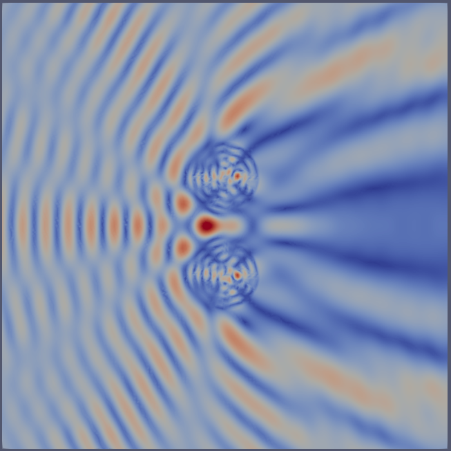
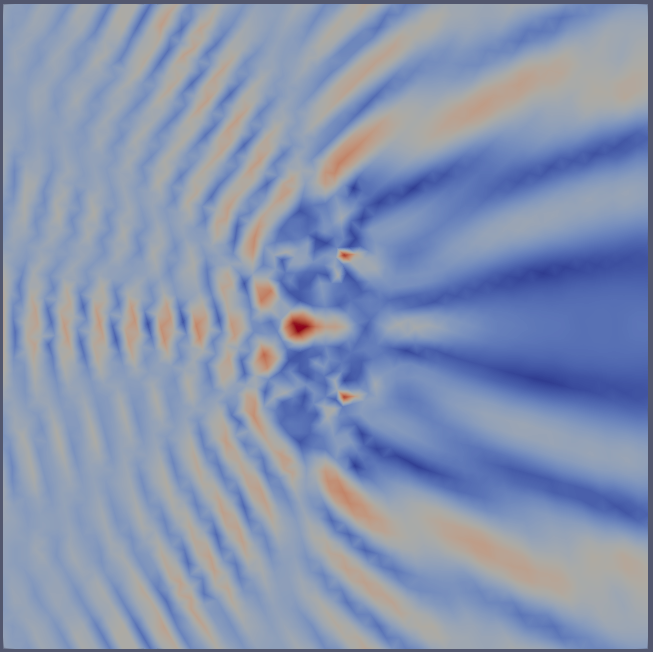
The Helmholtz equation
In this tutorial, we will learn:
- How to solve PDEs with complex-valued fields,
- How to import and use high-order meshes from Gmsh,
- How to use high order discretizations,
- How to use UFL expressions.
Problem statement
We will solve the Helmholtz equation subject to a first order absorbing boundary condition:
$$ \begin{align*} \Delta u + k^2 u &= 0 && \text{in } \Omega,\\ \nabla u \cdot \mathbf{n} - \mathrm{j}ku &= g && \text{on } \partial\Omega, \end{align*} $$where $k$ is a piecewise constant wavenumber, $\mathrm{j}=\sqrt{-1}$, and $g$ is the boundary source term computed as
$$g = \nabla u_\text{inc} \cdot \mathbf{n} - \mathrm{j}ku_\text{inc}$$for an incoming plane wave $u_\text{inc}$.
Interfacing with GMSH
In [4]:
from dolfinx.io import gmshio
from mesh_generation import generate_mesh

# MPI communicator
comm = MPI.COMM_WORLD

file_name = "domain.msh"
generate_mesh(file_name, lmbda, order=mesh_order)
mesh, cell_tags, _ = gmshio.read_from_msh(file_name, comm,
                                          rank=0, gdim=2)
Info    : Reading 'domain.msh'...
Info    : 15 entities
Info    : 2985 nodes
Info    : 1444 elements
Info    : Done reading 'domain.msh'
Material parameters
In [5]:
W = dolfinx.fem.FunctionSpace(mesh, ("DG", 0))
k = dolfinx.fem.Function(W)
k.x.array[:] = k0
k.x.array[cell_tags.find(1)] = 3 * k0
Boundary source term
$$g = \nabla u_{inc} \cdot \mathbf{n} - \mathrm{j}ku_{inc}$$where $u_{inc} = e^{-jkx}$, the incoming wave, is a plane wave propagating in the $x$ direction.
In [10]:
n = ufl.FacetNormal(mesh)
x = ufl.SpatialCoordinate(mesh)
uinc = ufl.exp(1j * k * x[0])
g = ufl.dot(ufl.grad(uinc), n) - 1j * k * uinc
Variational form
$$ -\int_\Omega \nabla u \cdot \nabla \bar{v} ~ dx + \int_\Omega k^2 u \,\bar{v}~ dx - j\int_{\partial \Omega} ku \bar{v} ~ ds = \int_{\partial \Omega} g \, \bar{v}~ ds \qquad \forall v \in \widehat{V}. $$
In [11]:
element = ufl.FiniteElement("Lagrange", mesh.ufl_cell(), degree)
V = dolfinx.fem.FunctionSpace(mesh, element)

u = ufl.TrialFunction(V)
v = ufl.TestFunction(V)
In [12]:
a = - ufl.inner(ufl.grad(u), ufl.grad(v)) * ufl.dx \
    + k**2 * ufl.inner(u, v) * ufl.dx \
    - 1j * k * ufl.inner(u, v) * ufl.ds
L = ufl.inner(g, v) * ufl.ds
Linear solver
In [13]:
opt = {"ksp_type": "preonly", "pc_type": "lu"}
problem = dolfinx.fem.petsc.LinearProblem(a, L, petsc_options=opt)
uh = problem.solve()
uh.name = "u"
Post-processing with Paraview
In [18]:
from dolfinx.io import XDMFFile, VTXWriter
u_abs = dolfinx.fem.Function(V, dtype=np.float64)
u_abs.x.array[:] = np.abs(uh.x.array)
XDMFFile
In [19]:
# XDMF writes data to mesh nodes
with XDMFFile(comm, "out.xdmf", "w") as file:
    file.write_mesh(mesh)
    file.write_function(u_abs)
VTXWriter
In [20]:
# VTX can write higher order functions
with VTXWriter(comm, "out_high_order.bp", [u_abs]) as f:
    f.write(0.0)