The Stokes equations
\begin{align*}
-\Delta \mathbf{u} + \nabla p &= \mathbf{f} &&\text{in } \Omega,\\
\nabla \cdot \mathbf{u} &= 0 &&\text{in } \Omega,\\
\mathbf{u} &= \mathbf{0}&&\text{on } \partial\Omega.
\end{align*}
In this tutorial you will learn how to:
- Create manufactured solutions with UFL
- Use block-preconditioners
Defining a manufactured solution
In [4]:
def u_ex(x):
    sinx = sin(pi * x[0])
    siny = sin(pi * x[1])
    cosx = cos(pi * x[0])
    cosy = cos(pi * x[1])
    c_factor = 2 * pi * sinx * siny
    return c_factor * as_vector((cosy * sinx, - cosx * siny))

def p_ex(x):
    return sin(2 * pi * x[0]) * sin(2 * pi * x[1])
In [5]:
def source(x):
    u, p = u_ex(x), p_ex(x)
    return - div(grad(u)) + grad(p)
Defining the variational form
$$\begin{align}
A w &= b,\\
\begin{pmatrix}
A_{\mathbf{u},\mathbf{u}} & A_{\mathbf{u},p} \\
A_{p,\mathbf{u}} & 0
\end{pmatrix}
\begin{pmatrix} u\\ p \end{pmatrix}
&= \begin{pmatrix}\mathbf{f}\\ 0 \end{pmatrix}
\end{align}$$
In [6]:
def create_bilinear_form(V, Q):
    u, p = TrialFunction(V), TrialFunction(Q)
    v, q = TestFunction(V), TestFunction(Q)
    a_uu = inner(grad(u), grad(v)) * dx
    a_up = inner(p, div(v)) * dx
    a_pu = inner(div(u), q) * dx
    return fem.form([[a_uu, a_up], [a_pu, None]])
In [7]:
def create_linear_form(V, Q):
    v, q = TestFunction(V), TestFunction(Q)
    domain = V.mesh
    x = SpatialCoordinate(domain)
    f = source(x)
    return fem.form([inner(f, v) * dx,
                     inner(fem.Constant(domain, 0.), q) * dx])
Create a block preconditioner
In [10]:
def create_preconditioner(Q, a, bcs):
    p, q = TrialFunction(Q), TestFunction(Q)
    a_p11 = fem.form(inner(p, q) * dx)
    a_p = fem.form([[a[0][0], None],
                    [None, a_p11]])
    P = fem.petsc.assemble_matrix_nest(a_p, bcs)
    P.assemble()
    return P
Assemble the nested system
In [11]:
def assemble_system(lhs_form, rhs_form, bcs):
    A = fem.petsc.assemble_matrix_nest(lhs_form, bcs=bcs)
    A.assemble()

    b = fem.petsc.assemble_vector_nest(rhs_form)
    fem.petsc.apply_lifting_nest(b, lhs_form, bcs=bcs)
    for b_sub in b.getNestSubVecs():
        b_sub.ghostUpdate(addv=PETSc.InsertMode.ADD,
                          mode=PETSc.ScatterMode.REVERSE)
    spaces = fem.extract_function_spaces(rhs_form)
    bcs0 = fem.bcs_by_block(spaces, bcs)
    fem.petsc.set_bc_nest(b, bcs0)
    return A, b
PETSc Krylov Subspace solver
In [12]:
def create_block_solver(A, b, P, comm):
    ksp = PETSc.KSP().create(comm)
    ksp.setOperators(A, P)
    ksp.setType("minres")
    ksp.setTolerances(rtol=1e-9)
    ksp.getPC().setType("fieldsplit")
    ksp.getPC().setFieldSplitType(PETSc.PC.CompositeType.ADDITIVE)

    nested_IS = P.getNestISs()
    ksp.getPC().setFieldSplitIS(("u", nested_IS[0][0]),
                                ("p", nested_IS[0][1]))

    # Set the preconditioners for each block
    ksp_u, ksp_p = ksp.getPC().getFieldSplitSubKSP()
    ksp_u.setType("preonly")
    ksp_u.getPC().setType("gamg")
    ksp_p.setType("preonly")
    ksp_p.getPC().setType("jacobi")

    # Monitor the convergence of the KSP
    ksp.setFromOptions()
    return ksp
Solving the Stokes problem with a block-preconditioner
In [14]:
def solve_stokes(u_element, p_element, domain):
    V = fem.FunctionSpace(domain, u_element)
    Q = fem.FunctionSpace(domain, p_element)

    lhs_form = create_bilinear_form(V, Q)
    rhs_form = create_linear_form(V, Q)

    bcs = create_velocity_bc(V)
    nsp = create_nullspace(rhs_form)
    A, b = assemble_system(lhs_form, rhs_form, bcs)
    assert nsp.test(A)
    A.setNullSpace(nsp)

    P = create_preconditioner(Q, lhs_form, bcs)
    ksp = create_block_solver(A, b, P, domain.comm)

    u, p = fem.Function(V), fem.Function(Q)
    w = PETSc.Vec().createNest([u.vector, p.vector])
    ksp.solve(b, w)
    assert ksp.getConvergedReason() > 0
    u.x.scatter_forward()
    p.x.scatter_forward()
    return compute_errors(u, p)
Crouzeix-Raviart
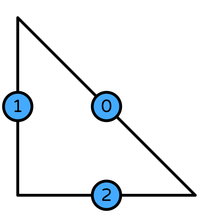

In [18]:
element_u = VectorElement("CR", "triangle", 1)
element_p = FiniteElement("DG", "triangle", 0)
error_plot(element_u, element_p, 1)

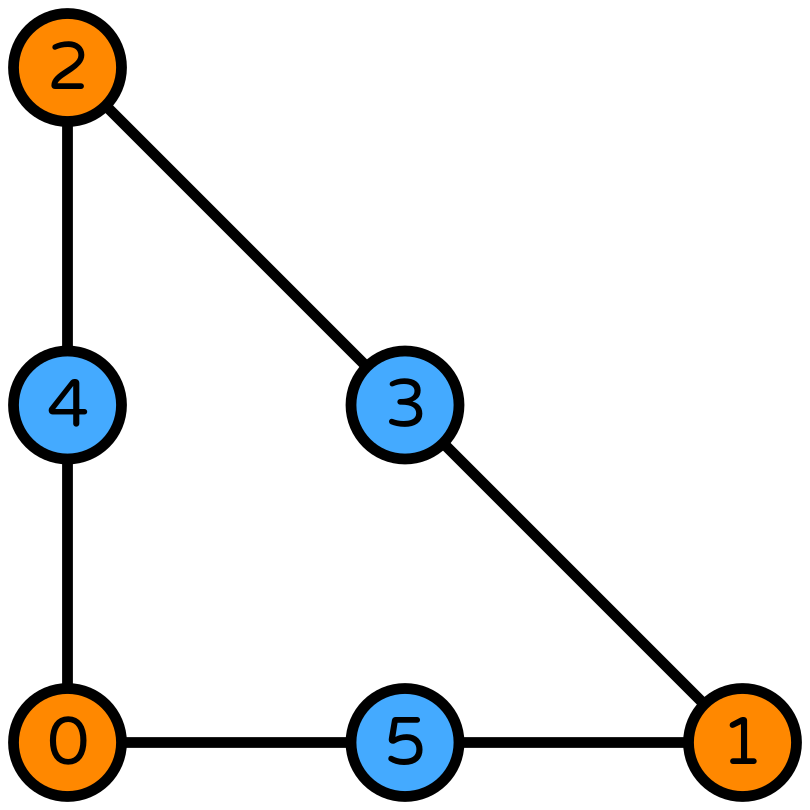
Piecewise linear pressure space

In [19]:
enriched_element = (
    FiniteElement("Lagrange", "triangle", 2)
    + FiniteElement("Bubble", "triangle", 3))
element_u = VectorElement(enriched_element)
element_p = FiniteElement("DG", "triangle", 1)
error_plot(element_u, element_p, 2)

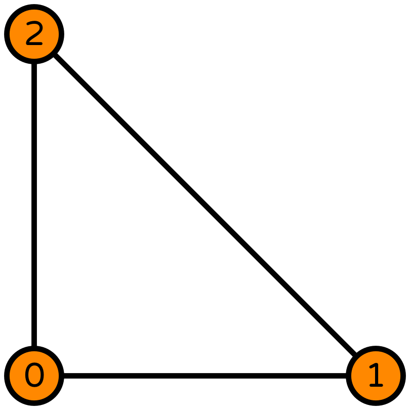
Taylor-Hood Element

In [24]:
element_u = VectorElement("CG", "triangle", 3)
element_p = FiniteElement("CG", "triangle", 2)
error_plot(element_u, element_p, 3)
