class: center, middle, inverse, title-slide .title[ # Lecture 07 ] .subtitle[ ## Policymaking Under Uncertainty ] .author[ ### Ivan Rudik ] .date[ ### AEM 4510 ] --- exclude: true ``` r if (!require("pacman")) install.packages("pacman") ``` ``` ## Loading required package: pacman ``` ``` r pacman::p_load( tidyverse, xaringanExtra, rlang, patchwork, nycflights13 ) source("R/video_helpers.R") options(htmltools.dir.version = FALSE) knitr::opts_hooks$set(fig.callout = function(options) { if (options$fig.callout) { options$echo <- FALSE } knitr::opts_chunk$set( cache = TRUE, cache.extra = list(tools::md5sum("R/video_helpers.R")), echo = TRUE, fig.align = "center" ) options }) ``` ``` ## Warning in xaringanExtra::style_panelset(panel_tab_color_active = "red"): 'xaringanExtra::style_panelset' is deprecated. ## Use 'style_panelset_tabs' instead. ## See help("Deprecated") ``` ``` ## Warning in style_panelset_tabs(...): The argument names of `style_panelset()` ## changed in xaringanExtra 0.1.0. Please refer to the documentation to update to ## the latest names. ``` ``` ## NULL ``` --- # Roadmap 1. Motivating examples of environmental uncertainty 2. Weitzman: taxes versus standards under MD and MAC uncertainty 3. Manne–Richel: abatement today under uncertainty about the future --- class: inverse, center, middle name: uncertainty # Uncertainty and the environment <html><div style='float:left'></div><hr color='#EB811B' size=1px width=796px></html> --- # Learning about arctic sea ice <video width="900" controls preload="metadata" style="display:block;margin:auto;" onplay="document.querySelectorAll('video').forEach(v => { if (v !== this) v.pause(); });"><source src="videos/07-uncertainty-arctic-sea-ice.mp4" type="video/mp4"><track kind="captions" src="videos/07-uncertainty-arctic-sea-ice.en.vtt" srclang="en" label="English" default></video> --- # Uncertainty in marginal damages It is very likely that we don’t know much about how damaging a particular pollutant is¹ .footnote[ ¹This is even ignoring the fact that we probably don't even know the slope of the marginal damage curve ] -- What are the actual health effects? -- Who are affected? -- Given health effects and affected groups, how do we value lives/health? -- How do we value threatened environmental amenities? --- # Climate change .pull-left[ <center> <img src="files/09-climate-sens.png" alt="" width="100%" /> </center> ] .pull-right[ These are our best estimates of the distribution of the .hi[equilibrium climate sensitivity:] how much the earth warms on average if we double CO₂ concentrations Uncertainty in ECS means we are uncertain about the true costs of emitting a ton of CO₂ (the social cost of CO₂) ] --- # Climate change .pull-left[ <center> <img src="files/09-damages.png" alt="" width="100%" /> </center> Rudik (2020) ] .pull-right[ There's also uncertainty over how costly a given amount of warming will be - How bad is 1 degree of warming for agricultural yields? These are distributions of damages to global GDP at given levels of warming ] --- # Uncertainty Uncertainty can factor into environmental policy-making in a number of ways: -- - Uncertainty in marginal damages (MD) -- - Uncertainty in marginal abatement costs (MAC) The type of uncertainty can have implications for instrument choice --- # Policy under uncertainty .pull-left[  ] .pull-right[ With .hi[perfect information] we can achieve the efficient outcome using either a tax `\(\tau\)` or an emission standard `\(\bar{E} = E^*\)` Will this hold true even with uncertainty about MD or MAC? ] --- # Policy under MD uncertainty <style> /* Each pause replaces the graph while retaining the paragraphs already shown. */ .md-uncertainty-step:has(~ .md-uncertainty-step), .mac-uncertainty-step:has(~ .mac-uncertainty-step) { display: none; } </style> .md-uncertainty-step[ .pull-left[  ] .pull-right[ If we are uncertain about MD how should we set policy? Suppose we have a best estimate, `\(MD_e\)` ] ] -- .md-uncertainty-step[ .pull-left[  ] .pull-right[ If we are uncertain about MD how should we set policy? Suppose we have a best estimate, `\(MD_e\)` Unfortunately our estimate was wrong, and the true MD curve is given by `\(MD_h\)` or `\(MD_l\)` ] ] -- .md-uncertainty-step[ .pull-left[  ] .pull-right[ If we are uncertain about MD how should we set policy? Suppose we have a best estimate, `\(MD_e\)` Unfortunately our estimate was wrong, and the true MD curve is given by `\(MD_h\)` or `\(MD_l\)` Let's say the actual MD is `\(MD_l\)`, what happens under our policies? ] ] --- # Policy under MD uncertainty .pull-left[  ] .pull-right[ First: what tax and standard does the regulator set? ] --- # Policy under MD uncertainty .pull-left[  ] .pull-right[ First: what tax and standard does the regulator set? The regulator selects a standard where she thinks MAC = MD: E_e The regulator selects a tax where she thinks MAC = MD: `\(\tau\)`_e With these two policies in place, what does the firm do? ] --- # Policy under MD uncertainty .pull-left[  ] .pull-right[ The firm emits at E_e under both the tax and standard We get the same outcome Is there any deadweight loss? If so, how much? ] --- # Policy under MD uncertainty .pull-left[  ] .pull-right[ We actually want to be at E^* We are emitting too little because we overestimated damages What is the DWL associated with under-emission? ] --- # Policy under MD uncertainty .pull-left[  ] .pull-right[ DWL comes from abatement costs in excess of the avoided damages This is the area in red With uncertain MD, we do not get the efficient outcome! ] --- # Policy under MAC uncertainty .mac-uncertainty-step[ .pull-left[  ] .pull-right[ Now suppose the regulator does not know the firms' .hi[MAC curves] The regulator's best estimate is `\(MAC_e\)` ] ] -- .mac-uncertainty-step[ .pull-left[ 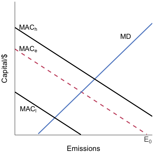 ] .pull-right[ Now suppose the regulator does not know the firms' .hi[MAC curves] The regulator's best estimate is `\(MAC_e\)` The true MAC may instead be `\(MAC_h\)` or `\(MAC_l\)` ] ] -- .mac-uncertainty-step[ .pull-left[ 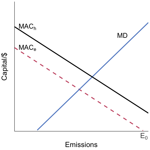 ] .pull-right[ Now suppose the regulator does not know the firms' .hi[MAC curves] The regulator's best estimate is `\(MAC_e\)` The true MAC may instead be `\(MAC_h\)` or `\(MAC_l\)` Suppose the true MAC is `\(MAC_h\)` ] ] --- # Policy under MAC uncertainty .pull-left[ 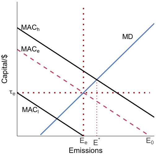 ] .pull-right[ The regulator again sets a standard of E_e and a tax of `\(\tau_e\)` We know the efficient level of emissions is E^* What level of emissions do we actually get? ] --- # Policy under MAC uncertainty .pull-left[  ] .pull-right[ Under a standard we get E_e ] --- # Policy under MAC uncertainty .pull-left[ 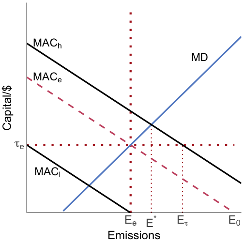 ] .pull-right[ Under a standard we get E_e Under a tax we get `\(E_\tau\)` Since we get different levels of emissions under the two policies, they may give us different levels of deadweight loss Let's see ] --- # Policy under MAC uncertainty .pull-left[  ] .pull-right[ The DWL under a standard is given by the .hi-red[red] area This is caused by .hi[too little emissions] ] --- # Policy under MAC uncertainty .pull-left[  ] .pull-right[ The DWL under a standard is given by the .hi-red[red] area This is caused by .hi[too little emissions] The DWL under a tax is given by the .hi-blue[blue] area This is caused by .hi[too many emissions] ] --- # Policy under MAC uncertainty .pull-left[  ] .pull-right[ The DWLs are similar-ish in size Why do we get the DWLs? ] --- # Policy under MAC uncertainty .pull-left[  ] .pull-right[ .hi[Standard:] we under estimated the MAC and thought it'd be cheaper to abate than it actually was, so we set too stringent of a standard .hi[Tax:] we under estimated the MAC and thought it'd be cheaper to abate than it actually was, so we set too low of a tax The same error leads to different qualitative outcomes ] --- # Policy under MAC uncertainty .pull-left[  ] .pull-right[ Which policy performs better depends on the relative slopes of the MAC and MD curves Now consider an example where the MD curve is relatively .hi[steep] Try to solve for the policy choices and DWLs yourself ] --- # Policy under MAC uncertainty .pull-left[  ] .pull-right[ If the MD curve is relatively steep a standard performs better, the .hi-red[red] DWL is smaller than the .hi-blue[blue] DWL Why? Taxes allow firms to choose the quantity If the MD is relatively steep, an error in the quantity of emissions is very costly ] --- # Steep MDs A steep MD means the marginal external cost of emissions increases rapidly -- Any examples? -- One would be if there exist .hi[tipping points] in the climate system: - Melt-back of Arctic summer sea ice - Evidence that this is happening even without much additional warming - Sea ice reflects light and cools polar regions - This has big effects on air and ocean circulation Collapse of Greenland ice sheet: could lead to a 7m rise in sea level --- # Policy under MAC uncertainty .pull-left[  ] .pull-right[ If MD is .hi[perfectly steep], the efficient quantity is pinned down exactly The standard still gives `\(E_e = E^*\)`, so there is .hi[no DWL under the standard] The tax still lets emissions move to `\(E_\tau\)` when MAC is higher than expected ] --- name: perfectly-steep-intuition # Perfectly steep MD and instrument choice If MD is .hi[perfectly steep], damages spike at `\(E^*\)`, so we do not need to know MAC to identify the efficient quantity A .hi[standard] set at `\(E^*\)` pins down emissions at the efficient quantity -- Under a .hi[tax], firms choose emissions where `\(MAC = \tau\)`, so unknown MAC prevents us from reliably hitting `\(E^*\)` -- The tax can cause .hi[too much abatement], or .hi[too little abatement] and emissions beyond the damage threshold, potentially causing catastrophic damages --- # Tipping points Collapse of western Antarctic ice sheet - Potential for immediate sea level rise -- Die-back of Amazonian rainforest - Species loss - Effects on rainfall patterns in other parts of the world -- Collapse of West African monsoon season and many others --- # Policy under MAC uncertainty .pull-left[  ] .pull-right[ Now what if MD is very flat? Solve for the regulator's chosen policies and their associated DWL ] --- # Policy under MAC uncertainty .pull-left[  ] .pull-right[ If the MD curve is relatively flat a tax performs better, the .hi-blue[blue] DWL is smaller than the .hi-red[red] DWL Why? ] --- # Policy under MAC uncertainty .pull-left[  ] .pull-right[ Marginal damages are relatively constant no matter the quantity while abatement costs can change rapidly It's valuable to let the firm flexibly choose abatement Taxes impose a constant incentive on the firm, closer representation of the MD ] --- # Policy under MAC uncertainty .pull-left[  ] .pull-right[ If MD is .hi[perfectly flat], the efficient price is pinned down exactly The tax still gives `\(\tau_e = MD\)`, so the firm chooses `\(E_\tau = E^*\)` There is .hi[no DWL under the tax], while the standard still fixes the wrong quantity ] --- name: perfectly-flat-intuition # Perfectly flat MD and instrument choice If MD is .hi[perfectly flat], the marginal external cost of emissions is known and constant, so we do not need to know MAC to identify the efficient price A .hi[tax] set at `\(\tau = MD\)` makes the firm pay that cost and choose `\(MAC = MD\)`, even though the regulator does not know MAC -- Under a .hi[standard], the implicit marginal price of emissions is MAC at the allowed quantity and depends on the firm's unknown MAC -- The implicit price can be .hi[too high or too low] relative to MD, so the standard can cause .hi[too much or too little abatement] --- # The Manne-Richel model Two periods (current and future) -- Two possible states of nature in the future (“good” with probability (1-p) and “bad” with probability p) -- In the bad state, the climate is .hi[very] sensitive to greenhouse gases; in the good state, it is less sensitive -- Each state requires different abatement to avoid climate catastrophe | State | Probability | Cumulative Abatement Required | |------- |:-------------: |:-------------------------------: | | Good | 1-p | 0 | | Bad | p | 1 | --- # The Manne-Richel model Greenhouse gases are stock pollutants -- Since greenhouse gases are very long-lived, abatement activity is cumulative (doing abatement activity today is as good as doing abatement activity in the future) -- a₁: current abatement a₂: future abatement a₁+a₂: aggregate abatement --- # The Manne-Richel model If we do a₁ units of abatement today in the future we need to do: -- 1 - a₁ units with probability p (bad state) -- 0 with probability 1-p (good state) -- Suppose abatement cost is given by: `\(C(a) = 0.5 a^2\)` -- What is the regulator's problem? --- # The Manne-Richel model `$$\min_{a_1} E[TC] = \underbrace{\frac{1}{2}a_1^2}_{\text{current cost}} + (1-p)\times \underbrace{0}_{\text{good state cost}} + p \times \underbrace{\frac{1}{2}(1-a_1)^2}_{\text{bad state cost}}$$` -- The first-order condition is: `$$\frac{d E[TC]}{da_1} = a^*_1 - p(1-a^*_1) = 0$$` -- This gives us that: `$$a^*_1 = \frac{p}{1+p}$$` --- # The Manne-Richel model `$$a^*_1 = \frac{p}{1+p}$$` If there is any chance of a bad state (p > 0), it is optimal to do *some* abatement today -- If a bad state is guaranteed (p = 1), we want `\(a^*_1 = 1/2, a^*_2 = 1/2\)` -- You can think about this as basically buying insurance --- # The Manne-Richel model It makes sense to do some abatement today, even if we are not sure there will be bad climate change, because the MAC is cheap for the first few units -- In marginal terms: we want to equate the MAC today with the *expected* MAC in the future so that on average, we can't reallocate abatement and be better off -- `$$a^*_1 = p(1-a^*_1)$$`