Modelling
Reporting, summarising and communicating models in R
Last session we talked a bit about how you might scrape data from the web. Collecting data is not an end in itself, rather the first step in answering your research question. When it comes to analysing trends, testing hypotheses, and predicting outcomes, modelling enters the picture. In this session, we won’t focus on the statistical considerations that inform your model choice, but rather show you how to:
- Use formulas to specify multiple models
- Process (estimate) model results with
broom - Summarise outputs with
modelsummary - Communicate results through plots and tables
The Model Workflow with R
While the last session dealt with one of the flashier aspects of data science (Web-Scraping), today we will return to the bread and butter 🍞 of any dedicated data scientist’s tool kit - modelling!
But if we aren’t even talking about Machine Learning, Deep Learning or model choice, why bother? Well, as with most things, it is worth revisiting fundamentals from time to time. By investing just a little more effort here, we can create much better reports and papers!
In general, remember that your basic workflow for evaluating and reporting models is as follows:
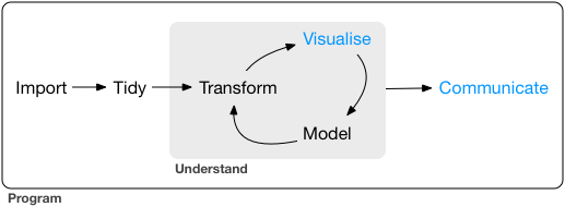
Today we will mostly deal with the “Model” and “Communicate” steps shown in the graph.
Setup
Before we start coding, we need to load several packages as well as our data. We’ll be using data from the World Health Organization on life expectancy.
# load packages
pacman::p_load(kableExtra, tidyverse, broom, modelsummary, specr, janitor, modelr, wesanderson)

# load data
life_expec_dat <- read_csv("life_expectancy.csv") |>
  janitor::clean_names() |>
  mutate(large = if_else(population > 50000000, 1, 0))  # pop size > 50M
head(life_expec_dat)
Using Formulas in R 👨🏫
R, as a programming language, was specifically designed with
statistical analysis in mind. Therefore the founding fathers of R 🙌 -
in their infinite wisdom - decided to create a special object class
(called formula) to help with running models.
Syntax
A quick recap of the syntax used within formulas. The ~
sign generally differentiates between dependent and independent
variables. The + sign is used to distinguish between
independent variables. Here are a few more common formula inputs that
are useful to know:
y ~ x1 + x2 # standard formula

y ~ . # include all other columns in data as x vars

y ~ x1 * x2 # interaction terms

y ~ x + I(x^2) # higher order terms
Formulas are generally straightforward to work with. To avoid any potential errors, you should follow these two steps:
Step 1: Create a string containing the written formula.
## [1] "life_expectancy ~ gdp"Step 2: Transform the string into R’s
formula class. Only then will your modeling function accept
it as input.
## life_expectancy ~ gdpHere is the proof that both ways of doing it are identical.
reg1 <- lm(form, data = life_expec_dat)
reg2 <- lm(life_expectancy ~ gdp, data = life_expec_dat)

reg1$coefficients == reg2$coefficients
## (Intercept) gdp
## TRUE TRUEIteration
We encourage you to fit many models, ranging from simple to complex. Formulas can help with making this process iterative.
Often, the modelling process requires you to run the same specification with multiple configurations of both dependent and independent variables. Model formulas make running many similar models much easier:
Step 1: Define a function that let’s you plug in
different variables for x or y. The function
should take the x and/or y variable(s) as a
string and return a model object.
# function to include different y variables
lm_fun_iter_y <-  function(dep_var) {
  lm(as.formula(paste(dep_var, "~ gdp")), data = life_expec_dat)
}

# function to include different x variables
lm_fun_iter_x <- function(indep_var) {
  lm(as.formula(paste("life_expectancy ~", paste(indep_var, collapse = "+"))), data = life_expec_dat)
}
Notice: Considering your model will
likely include many independent variables, it’s unlikely that you’ll run
a simple bivariate regression. Therefore, we need to use a nested paste
function that combines (with collapse()) all independent
variables contained in a character vector with +.
Step 2: Use map() (refer to lab
session 4) to iteratively apply the model to each variable contained
in a character vector of variables:
# create vector of variables to iterate over
vars <- life_expec_dat |>
  select(-c("life_expectancy", "country")) |>
  names()
vars
## [1] "year" "status"
## [3] "adult_mortality" "infant_deaths"
## [5] "alcohol" "percentage_expenditure"
## [7] "hepatitis_b" "measles"
## [9] "bmi" "under_five_deaths"
## [11] "polio" "total_expenditure"
## [13] "diphtheria" "hiv_aids"
## [15] "gdp" "population"
## [17] "thinness_1_19_years" "thinness_5_9_years"
## [19] "income_composition_of_resources" "schooling"
## [21] "large"## [[1]]
##
## Call:
## lm(formula = as.formula(paste("life_expectancy ~", paste(indep_var,
## collapse = "+"))), data = life_expec_dat)
##
## Coefficients:
## (Intercept) year
## -635.872 0.351
##
##
## [[2]]
##
## Call:
## lm(formula = as.formula(paste("life_expectancy ~", paste(indep_var,
## collapse = "+"))), data = life_expec_dat)
##
## Coefficients:
## (Intercept) statusDeveloping
## 79.2 -12.1
....This returns output from all of the models that you’ve just run.
Given that there are now quite a few models, it might be a good idea to
keep the names of the independent variables that you feed into the
model. You can do this with purrr::set_names().
# run a bivariate model for each column
biv_model_out_w_names <-  vars |>
  set_names() |>
  map(lm_fun_iter_x)

biv_model_out_w_names$year # we can now easily index independent vars
##
## Call:
## lm(formula = as.formula(paste("life_expectancy ~", paste(indep_var,
## collapse = "+"))), data = life_expec_dat)
##
## Coefficients:
## (Intercept) year
## -635.872 0.351Say that you’re interested in seeing what effect gdp has
on life_expectancy, but you suspect that other covariates
such as alcohol consumption, health care expenditure, average body mass
index and the propagation of aids also have an effect. On top of this,
it’s possible that these variables might have different affects on
life_expectancy depending on how they interact with each
other. We can determine which independent variables are robustly
associated with the dependent variable by generating models for every
possible combination of independent variables and then looking into the
distribution of effects across these models.
Let’s review the code introduced in the lecture:
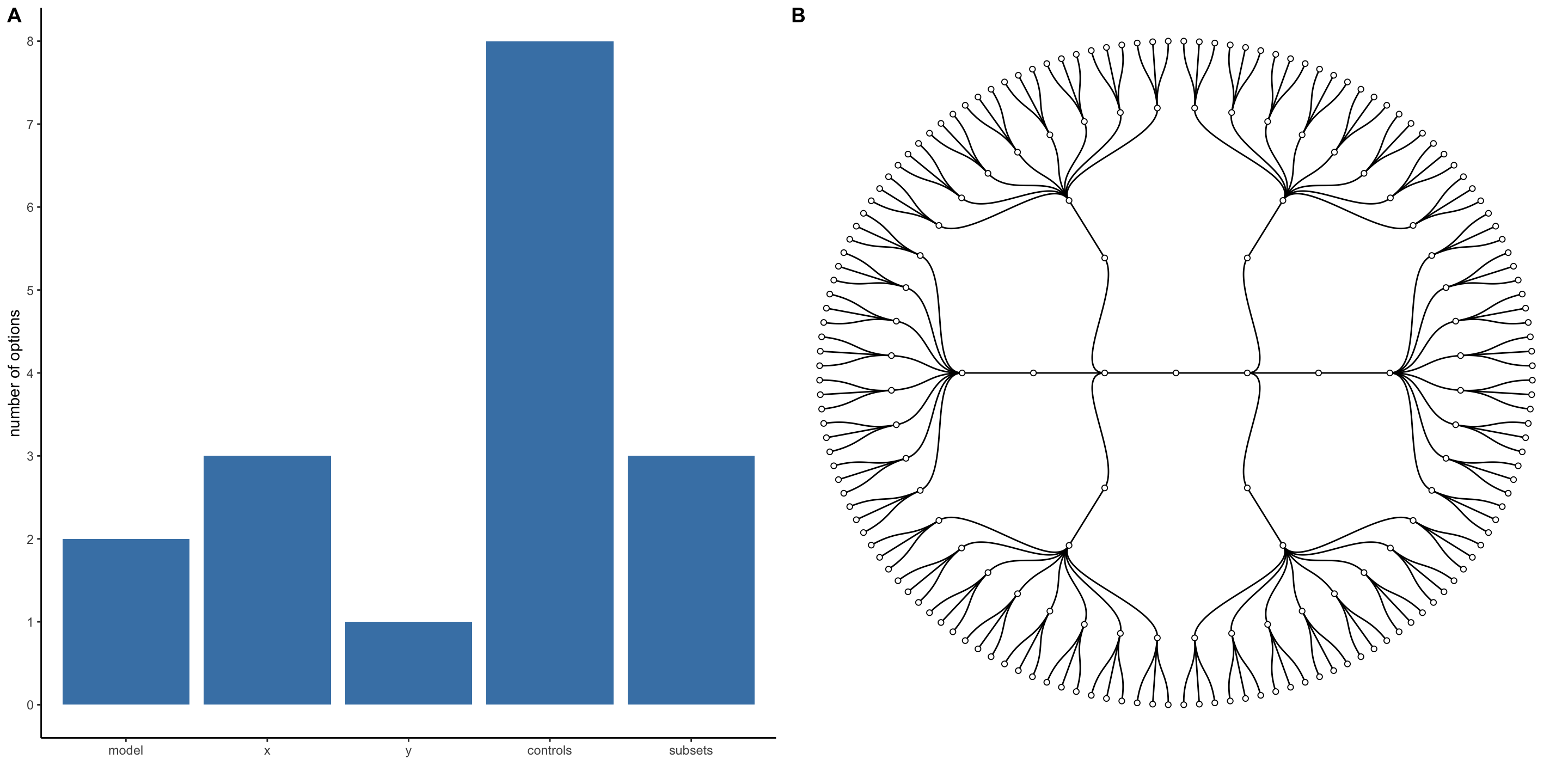
Step 1: Find out how many possible combinations of independent and dependent variables exist:
combinations <-
   map(1:5, function(x) {combn(1:5, x)}) |> # create all possible combinations (assume we have 5 covariates)
   map(ncol) |> # extract number of combinations
   unlist() |> # pull out of list structure
   sum() # compute sum
combinations
## [1] 31Step 2: Write a function that can run all possible combinations in one go:
combn_models <- function(depvar, covars, data) {

  # initialize empty list
  combn_list <- list()

  # generate list of covariate combinations
  for (i in seq_along(covars)) {
    combn_list[[i]] <- combn(covars, i, simplify = FALSE)
  } # what is combn?

  # unlist to make object easier to work with
  combn_list <-
    unlist(combn_list, recursive = FALSE)

  # function to generate formulas
  gen_formula <- function(covars, depvar) {
    form <-
      as.formula(paste0(depvar, " ~ ", paste0(covars, collapse = "+")))
    form
  }

  # generate formulas
  formulas_list <-
    purrr::map(combn_list, gen_formula, depvar = depvar)

  # run models
  models_list <- purrr::map(formulas_list, lm, data = data)
  models_list
}
Step 3: Apply the function to our case:
depvar <- "life_expectancy"
covars <-  c("gdp", "percentage_expenditure", "alcohol", "bmi", "hiv_aids")
multiv_model_out <- combn_models(depvar = depvar, covars = covars, data = life_expec_dat)

# check whether we have the correct number of models
length(multiv_model_out)
## [1] 31As you can see, the function introduced in the lecture is quite
powerful, but it is by no means the only option for testing multiple
model specifications. Depending on the type of analysis that you plan to
perform, certain R packages enable you run many different combinations
of regression models with just a few lines of code. For example, the we
can perform multiple
estimations with the fixest package.
Specification Curve Analysis ⤴️
In the example above, we consciously chose which models to run. Ideally, this decision should be grounded in theory and knowledge of the subject matter. Alternatively, some researchers argue that such choices are inherently arbitrary, potentially resulting in biased model specification. They propose taking a more analytical approach to model specification which they refer to as Specification Curve Analysis, or Multiverse Analysis.
We can implement this approach using the specr package.
In simple terms, it works as follows:
Step 1: Specify a list of reasonable “model ingredients” for each model parameter:
specs <- specr::setup(
  data = life_expec_dat,
  y = c("life_expectancy"), # add dependent variable
  x = c("gdp", "log(gdp)", "I(gdp^2)"), # add independent variables
  model = c("lm", "glm"), # specify model types
  controls = c("population", "alcohol", "bmi"), # specify controls
  as.list(distinct(life_expec_dat, status)) # specify subgroup
  )

summary(specs, rows = 20)
## Setup for the Specification Curve Analysis
## -------------------------------------------
## Class: specr.setup -- version: 1.0.0
## Number of specifications: 144
##
## Specifications:
##
## Independent variable: gdp, log(gdp), I(gdp^2)
## Dependent variable: life_expectancy
## Models: lm, glm
## Covariates: no covariates, population, alcohol, bmi, population + alcohol, population + bmi, alcohol + bmi, population + alcohol + bmi
## Subsets analyses: Developing, Developed, all
##
## Function used to extract parameters:
##
## function (x)
## broom::tidy(x, conf.int = TRUE)
## <environment: 0x10b045b28>
##
##
## Head of specifications table (first 20 rows):Step 2: Run Specification Curve Analysis:
Step 3: Inspect the specification curve to understand how robust your findings are to different analytical choices.
These plots help to illustrate where and when you had to make a choice and how many models you might alternatively have specified.
More concretely you could also look at some summary statistics for your p-values across the different model specifications:
Note that statistic mad stands for median absolute deviation.
A more intuitive way of inspecting the results might be to visualise them.
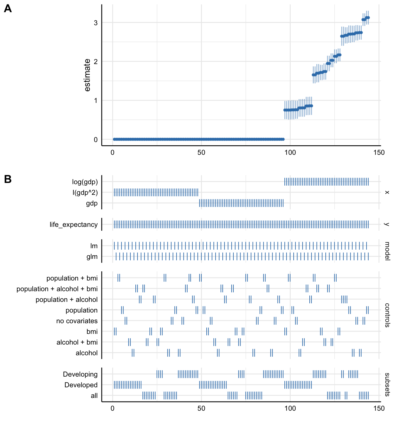
Plot A denotes:
- X-axis = ordered model specifications (from most negative effect to most positive effect)
- Y-axis = standardized regression coefficient for the IV-DV relationship
- Points = the standardized regression coefficient for each specific model
- Error bars = 95% confidence intervals around the point estimate
Plot B denotes:
- X-axis = ordered model specifications (the same as panel A)
- Y-axis (right) = analytic decision categories
- Y-axis (left) = specific analytic decisions within each category
- Lines = indicates whether a specific analytic decision was true for that particular model specification
Any comments on the above plot? 🤔
Interpretable Effect Sizes 🔎
While these plots make it easy to compare effects across coefficients, unit changes may not be comparable across variables. We can address this problem in several ways:
- Re-scale variables to show intuitive unit changes in X (e.g., $1k instead of $1)
- Re-scale to full scale (minimum to maximum) changes in X
- Standardise variables to show standard deviation changes in X
Let’s try standardising our variables to address the problem.
# copy our data
life_expec_dat_stand <- life_expec_dat

# standardise  variables
life_expec_dat_stand <- life_expec_dat_stand |>
  mutate(gdp = effectsize::standardise(gdp))

# specify reasonable model "ingredients"
specs_stand <- specr::setup(
  data = life_expec_dat_stand,
  y = c("life_expectancy"), # add dependent variable
  x = c("gdp", "log(gdp)", "I(gdp^2)"), # add independent variables
  model = c("lm", "glm"), # specify model types
  controls = c("population", "alcohol", "bmi"), # specify controls
  as.list(distinct(life_expec_dat_stand, status)) # specify subgroup
  )

# run specification curve analysis
results_stand <- specr::specr(specs_stand)

# plot entire visualization
plot(results_stand) 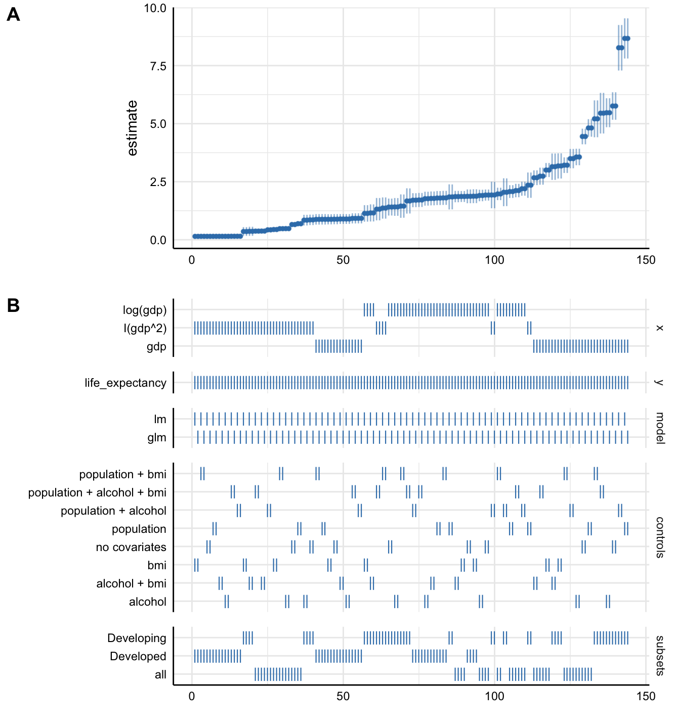
Note that any re-scaling operation will affect how you interpret the
coefficients! For more details, check out the effectsize
package.
Without putting much thought into our model, it looks like
gdp (depending on the specification) can either have a
small positive effect or a substantial positive effect on
life_expectancy. This just goes to show how
careful one has to approach the task of correctly
specifying a model!
Watch Out!
Be careful and selective when you use specification curve analysis! It is not a tool that you should apply to each and every potential paper. Especially, if you have not taken a course on causal inference. Specification curve analysis, when it includes variables that act as colliders or mediators, might actually legitimise an otherwise wrongly specified model!
Model Output with broom 🧹
In the lecture we saw that lists of different combinations of model specifications can be unwieldy. Simon also pointed out that we are interested in three main aspects of our model outputs:
- Estimated coefficients and associated standard errors, t-statistics, p-values, confidence intervals
- Model summaries including goodness of fit measures, information on model convergence, number of observations used
- Observation-level information that arises from the estimated model, such as fitted/predicted values, residuals, estimates of influence
Extracting this information from the model output is possible but not straightforward:
## List of 13
##  $ coefficients : Named num [1:2] 64.763 0.955
##   ..- attr(*, "names")= chr [1:2] "(Intercept)" "alcohol"
##  $ residuals    : Named num [1:2735] 0.227 -4.873 -4.873 -5.273 -5.573 ...
##   ..- attr(*, "names")= chr [1:2735] "1" "2" "3" "4" ...
##  $ effects      : Named num [1:2735] -3617.34 202.2 -4.78 -5.18 -5.48 ...
##   ..- attr(*, "names")= chr [1:2735] "(Intercept)" "alcohol" "" "" ...
##  $ rank         : int 2
##  $ fitted.values: Named num [1:2735] 64.8 64.8 64.8 64.8 64.8 ...
##   ..- attr(*, "names")= chr [1:2735] "1" "2" "3" "4" ...
....##
## Call:
## .f(formula = .x[[i]], data = ..1)
##
## Residuals:
## Min 1Q Median 3Q Max
## -33.96 -4.72 1.62 6.41 20.76
##
## Coefficients:
## Estimate Std. Error t value Pr(>|t|)
....Tidying Model Objects
Luckily, we don’t have to deal with this. We can use the tidyverse’s broom
package which is part of a collection of packages used for modeling that
adhere to tidyverse principles referred to as tidymodels. Tidymodels offers a
lot of cool packages that have their own tutorials, so check them out!
💪.
In today’s session, we will only focus on broom. As a
refresher, here are the three key broom functions that you should
know:
tidy(): Summarizes information about model components.
glance(): Reports information about the entire model.
augment(): Adds information about observations to a dataset.
Doesn’t this look so much tidier?
Broom with Many Models
Where broom really shines is when it comes to dealing
with multiple models like we have in our multiv_model_out.
It allows us to easily move away from hard-to-deal-with lists while
retaining each of the three important model outputs. Since our example
replicates several variables in different models, we include the
.id argument in map(). This adds a column to
our tibble which will contain a model identifier. In
our example, the identifier of each model corresponds with the index
number of the model output.
multiv_model_out_broom <- map_dfr(multiv_model_out[1:3],
                                  broom::tidy, .id = "model_type")
multiv_model_out_broom
Now that we have multiple model outputs in a format that we can work
with, it is time to start thinking about visualising our results. You
can plot the residuals, the goodness of fit statistics etc. Similarly,
you could also use glance() to provide some robustness
statistics or descriptive tables.
The next section will focus on how to present your results!
Results with modelsummary 🥼
For this we will use the modelsummary package by Vincent
Arel-Bundock’s. Though there are many packages to choose from when
it comes to communicating your results, we highly recommend you give
modelsummary a shot!
One reason that we like this package is that it combines both approaches of presenting model results, either as a table or as a coefficient plot. As we saw in the lecture, each method has its advantages and its drawbacks. Therefore, we will cover both here.
Using Regression Tables
The workhorse function in modelsummary is unsurprisingly
modelsummary(). 🤔
Here we only need to input the models list as the function does all of the tidying for us.
| (1) | |
|---|---|
| (Intercept) | 61.451 |
| (0.293) | |
| gdp | 0.000 |
| (0.000) | |
| percentage_expenditure | 0.000 |
| (0.000) | |
| alcohol | 0.394 |
| (0.034) | |
| bmi | 0.167 |
| (0.007) | |
| hiv_aids | −0.779 |
| (0.023) | |
| Num.Obs. | 2313 |
| R2 | 0.631 |
| R2 Adj. | 0.630 |
| AIC | 14787.7 |
| BIC | 14828.0 |
| Log.Lik. | −7386.873 |
| RMSE | 5.90 |
It looks pretty solid already, but can definitely be improved upon.
For example, we can set acceptable number of digits:
We can also report only the C.I. by getting rid of the p-values and intercept term:
model_table <- modelsummary(multiv_model_out[[31]],
             output = "kableExtra",
             fmt = "%.2f",  # 2-digits and trailing 0
             estimate  = "{estimate}",
             statistic = "conf.int",
             coef_omit = "Intercept")
Wouldn’t it look more professional if our coefficients began with capital letter? And how about we get rid of some of the bloated goodness of fit statistics?
mod_table <- modelsummary(multiv_model_out[31],
             output = "default",
             fmt = "%.2f",  # 2-digits and trailing 0
             estimate  = "{estimate}",
             statistic = "conf.int",
             coef_omit = "Intercept",
             coef_rename=c("gdp"="Gdp",
                           "bmi"="Avg. BMI",
                           "alcohol" = "Alcohol Consum.",
                           "hiv_aids"= "HIV cases",
                           "percentage_expenditure" = "Health Expenditure (% of GDP)",
                           "life_expectancy" = "Life Expectancy"),
             gof_omit = 'DF|Deviance|Log.Lik|AIC|BIC',
             title = 'A Most Beautiful Regression Table')
When using the kableExtra package, you can even
post-process your table:
mod_table |>
  kable_styling(bootstrap_options = c("striped", "hover", "condensed", "responsive"), full_width = F, fixed_thead = T) |>
  row_spec(3, color = 'red') |>
row_spec(5, background = 'lightblue')| (1) | |
|---|---|
| Gdp | 0.00 |
| [0.00, 0.00] | |
| Health Expenditure (% of GDP) | −0.00 |
| [−0.00, 0.00] | |
| Alcohol Consum. | 0.39 |
| [0.33, 0.46] | |
| Avg. BMI | 0.17 |
| [0.15, 0.18] | |
| HIV cases | −0.78 |
| [−0.82, −0.73] | |
| Num.Obs. | 2313 |
| R2 | 0.631 |
| R2 Adj. | 0.630 |
| RMSE | 5.90 |
Using Plots
If you are looking for an alternative way to present your results, you might also consider a nice coefficient plot 🎨
Again, modelsummary provides a very accessible function
for this: modelplot(). As with the regression table, you
input the Model List and not the tidied
output. The tidying happens under the hood.
# to avoid overplotting, we define a smaller list of models
models <- list(
  "Bivariate OLS" = lm(life_expectancy ~ gdp, data = life_expec_dat),
  "Multivariate OLS" = lm(life_expectancy ~ gdp + total_expenditure + population + alcohol + bmi, data = life_expec_dat),
  "Interaction" = lm(life_expectancy ~  gdp + total_expenditure + population + gdp*total_expenditure, data = life_expec_dat),
  "Polynomial" = lm(life_expectancy ~ gdp + I(gdp^2), data = life_expec_dat)
  )

# plot
modelplot(models, coef_omit = "Intercept") 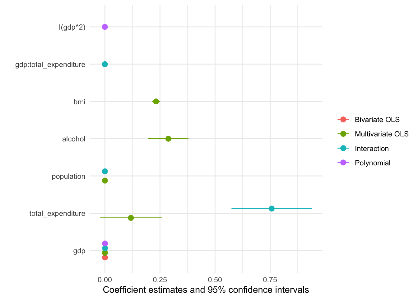
Now we just need to customise the plot to our liking:
modelplot(models, coef_omit = "Intercept") +
    labs(x = 'Coefficients',
         y = 'Term names',
         title = 'Linear regression models of "Life expectancy"',
caption = "Comparing multiple models, the data originated at the WHO") 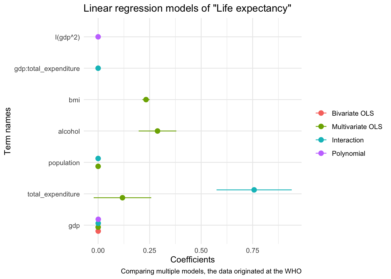
We will cover data visualisation with R in much greater detail in the next session, so hopefully the section on coefficient plot will be made clearer then!
Appendix
Crafting formulas
The basic structure of a formula:
## y ~ xRunning a model with a formula is straightforward. Note that we don’t even have to put the formula in parentheses:
##
## Call:
## lm(formula = arr_delay ~ distance + origin, data = flights)
##
## Coefficients:
## (Intercept)     distance    originJFK    originLGA
##    13.41405     -0.00405     -2.70426     -4.45617
A more explicit way to write formulas:
## [1] "formula"##
## Call:
## lm(formula = fmla, data = flights)
##
## Coefficients:
## (Intercept) distance originJFK originLGA
## 13.41405 -0.00405 -2.70426 -4.45617More formula syntax:
## y ~ x1 + x2## y ~ x1 - x2## y ~ .Interactions:
## y ~ x1 * x2## y ~ x1:x2As-is variables:
## y ~ x + I(x^2)Extract all variable names from a formula object:
## [1] "arr_delay" "distance" "origin"Incrementally modify/update a formula:
Further reading
Advanced crafting of formulas: fitting multiple models
Create a formula for a model with a large number of variables:
## y ~ x1 + x2 + x3 + x4 + x5 + x6 + x7 + x8 + x9 + x10 + x11 +
##     x12 + x13 + x14 + x15 + x16 + x17 + x18 + x19 + x20 + x21 +
##     x22 + x23 + x24 + x25
Create a multitude of covariate sets
Step 1: Define dependent variable + covariate set
Step 2: Build function to run lm models across set of all possible variable combinations
combn_models <- function(depvar, covars, data)
{
  combn_list <- list()
  # generate list of covariate combinations
  for (i in seq_along(covars)) {
    combn_list[[i]] <- combn(covars, i, simplify = FALSE)
  }
  combn_list <- unlist(combn_list, recursive = FALSE)
  # function to generate formulas
  gen_formula <- function(covars, depvar) {
    form <- as.formula(paste0(depvar, " ~ ", paste0(covars, collapse = "+")))
    form
  }
  # generate formulas
  formulas_list <- purrr::map(combn_list, gen_formula, depvar = depvar)
  # run models
  models_list <- purrr::map(formulas_list, lm, data = data)
  models_list
}
Step 3: Run models (careful, this’ll generate a quite heavy list)
## [1] 63Working with tidy model outputs
Inspecting models in R is straightforward with the
summary() function.
##
## Call:
## lm(formula = arr_delay ~ distance + origin, data = flights)
##
## Residuals:
##    Min     1Q Median     3Q    Max
##  -89.0  -24.0  -11.8    7.3 1281.4
##
## Coefficients:
##             Estimate Std. Error t value Pr(>|t|)
## (Intercept) 13.41405    0.17481    76.7   <2e-16 ***
## distance    -0.00404    0.00011   -36.9   <2e-16 ***
## originJFK   -2.70425    0.18871   -14.3   <2e-16 ***
## originLGA   -4.45617    0.19351   -23.0   <2e-16 ***
## ---
## Signif. codes:  0 '***' 0.001 '**' 0.01 '*' 0.05 '.' 0.1 ' ' 1
##
## Residual standard error: 44 on 327342 degrees of freedom
##   (9430 observations deleted due to missingness)
## Multiple R-squared:  0.0055, Adjusted R-squared:  0.00549
## F-statistic:  604 on 3 and 327342 DF,  p-value: <2e-16
But often you want to post-process estimation results. So let’s examine the output of a model function more closely.
Ugh, that’s a lot of information in a list structure. Let’s use some helper functions to unpack these:
We can also dig in the summary of the model.
##             Estimate Std. Error t value Pr(>|t|)
## (Intercept)   13.414    0.17481      77  0.0e+00
## distance      -0.004    0.00011     -37 5.5e-297
## originJFK     -2.704    0.18871     -14  1.5e-46
## originLGA     -4.456    0.19351     -23 3.0e-117
The broom philosophy 🧹
The broom package takes the messy output of built-in R functions such
as lm(), nls(), or t.test(), and
turns them into tidy tibbles.
Example: linear model output
##
## Call:
## lm(formula = arr_delay ~ distance + origin, data = flights)
##
## Coefficients:
## (Intercept)     distance    originJFK    originLGA
## 13.41405 -0.00405 -2.70426 -4.45617##
## Call:
## lm(formula = arr_delay ~ distance + origin, data = flights)
##
## Residuals:
## Min 1Q Median 3Q Max
## -89.0 -24.0 -11.8 7.3 1281.4
##
## Coefficients:
## Estimate Std. Error t value Pr(>|t|)
## (Intercept) 13.41405 0.17481 76.7 <2e-16 ***
## distance -0.00404 0.00011 -36.9 <2e-16 ***
## originJFK -2.70425 0.18871 -14.3 <2e-16 ***
## originLGA -4.45617 0.19351 -23.0 <2e-16 ***
## ---
## Signif. codes: 0 '***' 0.001 '**' 0.01 '*' 0.05 '.' 0.1 ' ' 1
##
## Residual standard error: 44 on 327342 degrees of freedom
## (9430 observations deleted due to missingness)
## Multiple R-squared: 0.0055, Adjusted R-squared: 0.00549
## F-statistic: 604 on 3 and 327342 DF, p-value: <2e-16Examine model object:
Inspect summary statistics:
Add fitted values and residuals to original data:
tidy() can also be applied to htest
objects:
The true power of broom unfolds in settings where you want to combine results from multiple analyses (using subgroups of data, different models, bootstrap replicates of the original data frame, permutations, imputations, …).
Step 4: (continuing the analysis from above): Extract results from all models
Step 5: Summarize results
models_broom_df |>
  filter(!str_detect(term, "Intercept|carrier")) |>
  ggplot(aes(estimate)) +
  geom_histogram(binwidth = .1) +
  geom_vline(xintercept = 0, linetype="dashed") +
  facet_grid(cols = vars(term), scales = "free_y") +
  theme_minimal()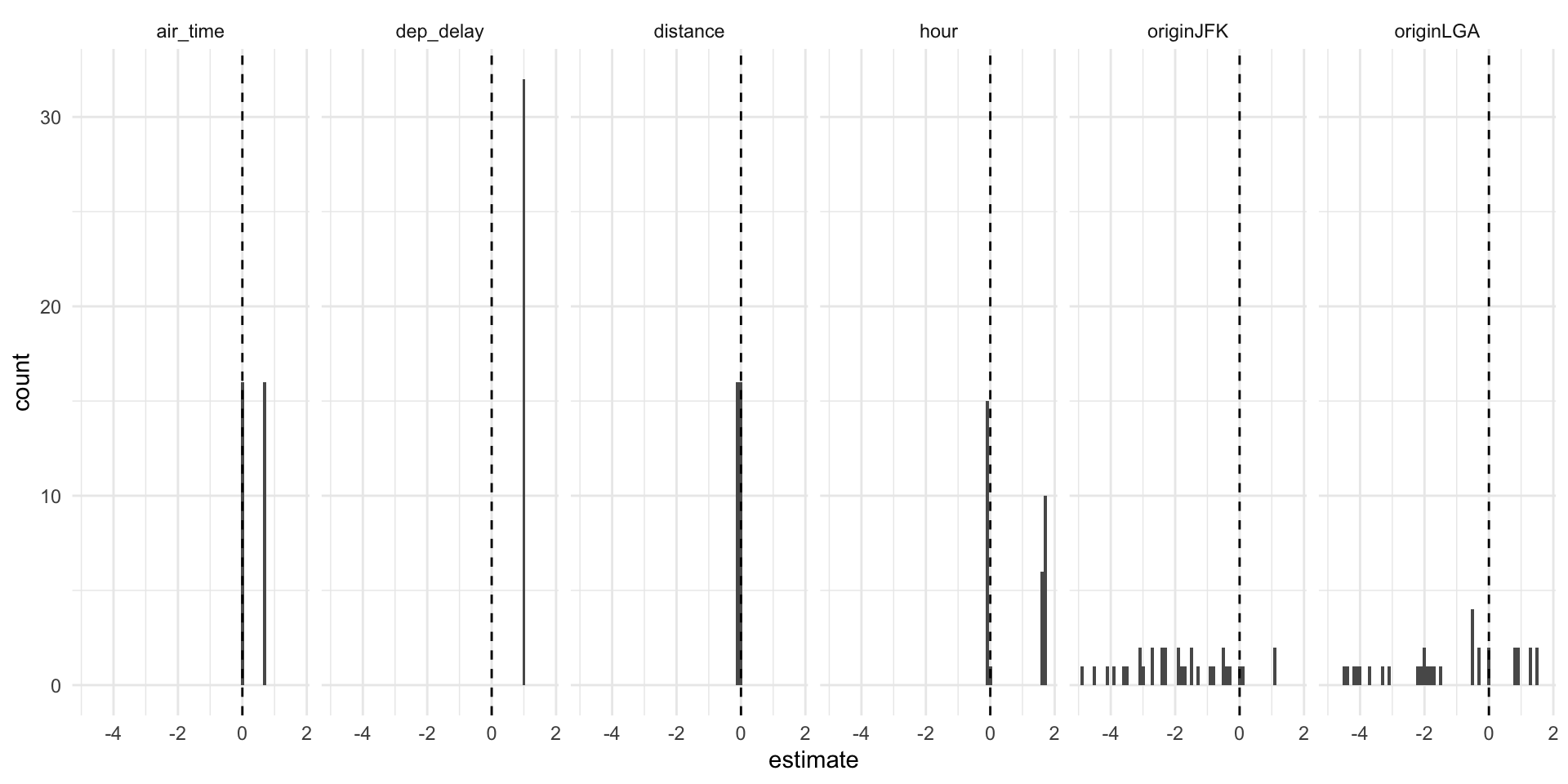
Further reading
Reporting model results
Tables
A table of models:
model1_out <- lm(arr_delay ~ dep_delay, data = flights)
model2_out <- lm(arr_delay ~ distance, data = flights)
model3_out <- lm(arr_delay ~ dep_delay + distance, data = flights)

models <- list(model1_out, model2_out, model3_out)

modelsummary(models,
             estimate = "{estimate} [{conf.low}, {conf.high}]",
             statistic = NULL,
             gof_omit = ".+",
title = "Linear regression of flight delay at arrival (in mins)") | (1) | (2) | (3) | |
|---|---|---|---|
| (Intercept) | −5.899 [−5.964, −5.835] | 10.829 [10.564, 11.095] | −3.213 [−3.322, −3.104] |
| dep_delay | 1.019 [1.018, 1.021] | 1.018 [1.017, 1.020] | |
| distance | −0.004 [−0.004, −0.004] | −0.003 [−0.003, −0.002] |
Coefficient plots
One model, one plot:
cm <- c("distance" = "Distance",
        "originLGA" = "Origin: LGA",
        "originJFK" = "Origin: JFK")
modelplot(model_out,
          coef_omit = "Interc",
          coef_map = cm)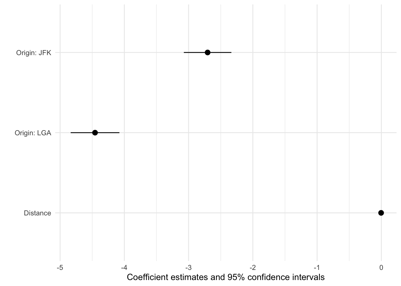
Standardised continuous variable:
flights$distance_std <- effectsize::standardize(flights$distance)
model_out_std2 <-lm(arr_delay ~ distance_std + origin, data = flights)
cm <- c("distance_std" = "Distance",
        "originLGA" = "Origin: LGA",
        "originJFK" = "Origin: JFK")
One model, one plot (more options):
modelplot(model_out_std2, coef_omit = "Interc", coef_map = cm) +
  xlim(-5, .25) +
  geom_vline(xintercept = 0, linetype="dashed") +
  labs(title = "Linear regression of flight delay at arrival (in mins)",
       caption = "Data source: nycflights13 package") +
  theme_minimal()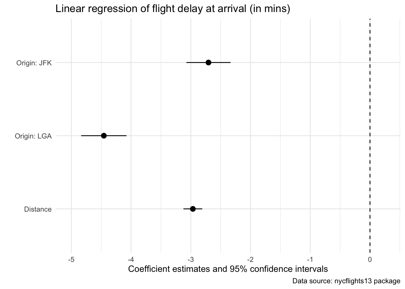
Re-scale continuous variable:
flights$distance1kmiles <- flights$distance / 1000
model_out_kmiles <-lm(arr_delay ~ distance1kmiles + origin, data = flights)
cm <- c("distance1kmiles" = "Distance (1k miles)",
        "originLGA" = "Origin: LGA",
        "originJFK" = "Origin: JFK")
One model, one plot (more options):
modelplot(model_out_kmiles, coef_omit = "Interc", coef_map = cm) +
  xlim(-5, .25) +
  geom_vline(xintercept = 0, linetype="dashed") +
  labs(title = "Linear regression of flight delay at arrival (in mins)",
       caption = "Data source: nycflights13 package") +
  theme_minimal()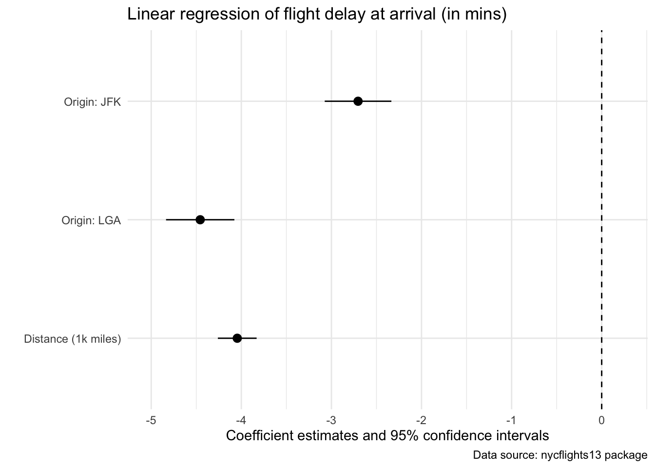
Multiple options, one faceted plot:
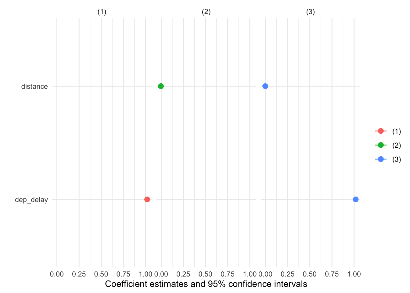
## Help on topic 'standardize' was found in the following packages:
##
##   Package               Library
##   datawizard            /Library/Frameworks/R.framework/Versions/4.3-arm64/Resources/library
##   effectsize            /Library/Frameworks/R.framework/Versions/4.3-arm64/Resources/library
##   mvtnorm               /Library/Frameworks/R.framework/Versions/4.3-arm64/Resources/library
##
##
## Using the first match ...True-vs-fitted plots
model_out |>
  augment() |>
  slice_sample(n = 10000) |>
  ggplot(aes(x = .fitted, y = arr_delay)) +
  geom_point(alpha =  0.25) +
  geom_abline(intercept = 0, slope = 1) +
  labs(title = "Fitted vs. true values, lm(arr_delay ~ distance + origin)",
       caption = "Data source: nycflights13 package") +
  xlab("Fitted values") +
  ylab("Arrival delay (in mins)") +
  theme_minimal()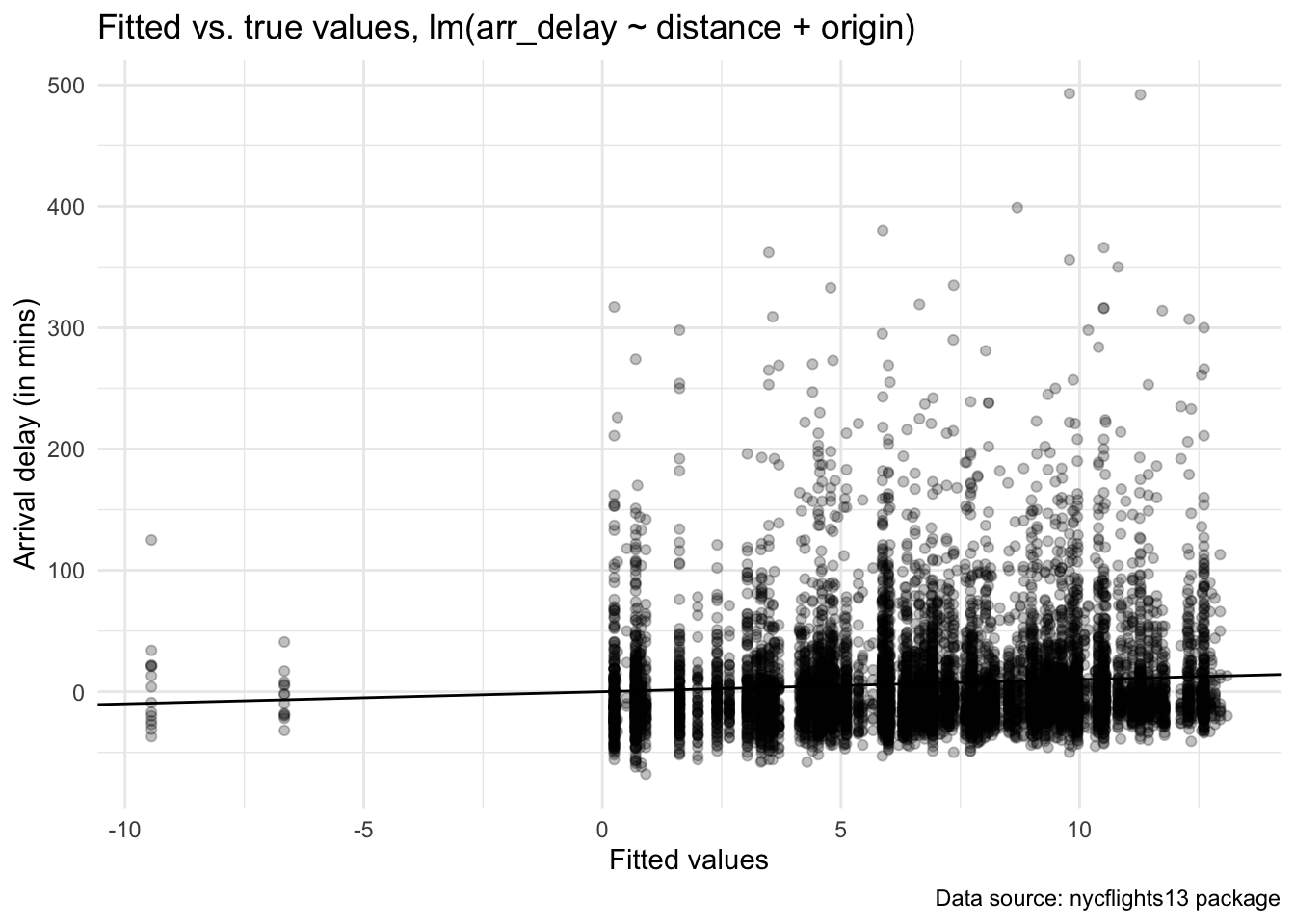
model_out_improve <- lm(arr_delay ~ dep_delay + distance + origin, data = flights)
model_out_improve |>
  augment() |>
  slice_sample(n = 10000) |>
  ggplot(aes(x = .fitted, y = arr_delay)) +
  geom_point(alpha =  0.25) +
  geom_abline(intercept = 0, slope = 1) +
  labs(title = "Fitted vs. true values, lm(arr_delay ~ dep_delay + distance + origin)",
       caption = "Data source: nycflights13 package") +
  xlab("Fitted values") +
  ylab("Arrival delay (in mins)") +
  theme_minimal()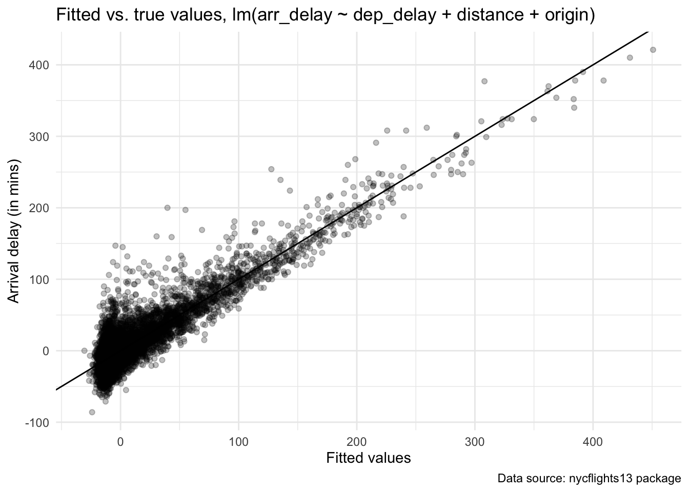
Further reading
- The
modelsummarypackage creates tables and plots to summarize statistical models and data in R - Alternative packages for model summaries, including stargazer and texreg
- Yet another alternative for data visualization for statistics: sjPlot
Sources
This tutorial drew heavily on the vignette from the specr package as well as the Regression Section in McDermott’s Data Science for Economists by Grant McDermott.
A work by Lisa Oswald & Tom Arend
Prepared for Intro to Data Science, taught by Simon Munzert