This week, we will teach you one of the most important parts of coding with R (and I cannot stress enough how important it is). Built-in functions and packages can only get you so far, there will be times when it is both easier and more efficient to create your own. Writing your own functions is a key skill in any coding language really, and R is no different. Unfortunately, writing your own function also requires you to be able to find and fix bugs that will inevitably creep into your code. For all of these reasons, this lab will teach you how to:

write your own functions
iterate functions over multiple inputs
vectorise your functions using the purrr package
debug your code

Quick review: lists 📃

One of the more important objects in R for functional programming are lists. Since we only briefly touched upon them in Week 1, let’s go over them again in more detail.

Vectors can only hold a single data type.

vec <- c(a = "hello", b = 1)

By comparison lists can hold many different data types at the same time.

list(a = "hello", b = 1, c = mean)

## $a
## [1] "hello"
## 
## $b
## [1] 1
## 
## $c
## function (x, ...) 
## UseMethod("mean")
## <bytecode: 0x0000000015643848>
## <environment: namespace:base>

When you think about, data.frames are also lists (or rather a list of columns).

library(gapminder)
head(gapminder)

You don’t believe me?

as.list(head(gapminder))

## $country
## [1] Afghanistan Afghanistan Afghanistan Afghanistan Afghanistan Afghanistan
## 142 Levels: Afghanistan Albania Algeria Angola Argentina Australia ... Zimbabwe
## 
## $continent
## [1] Asia Asia Asia Asia Asia Asia
## Levels: Africa Americas Asia Europe Oceania
## 
## $year
## [1] 1952 1957 1962 1967 1972 1977
## 
## $lifeExp
## [1] 28.801 30.332 31.997 34.020 36.088 38.438
## 
## $pop
## [1]  8425333  9240934 10267083 11537966 13079460 14880372
## 
## $gdpPercap
## [1] 779.4453 820.8530 853.1007 836.1971 739.9811 786.1134

Lists will be very common (and useful) once you get into the writing of your functions and iterating them using the purrr family of functions.

Functions 🏭

In any coding language a fundamental principle should be DRY (Don’t Repeat Yourself). You should adhere to this as much as possible, but really, once you have copy-pasted code twice, it is time to write a function.

Functions allow you to automate tasks in a more powerful and general way than copy-and-pasting. Writing a function has three big advantages over using copy-and-paste:

You can give a function an evocative name that makes your code easier to understand.
As requirements change, you only need to update code in one place, instead of many.
You eliminate the chance of making incidental mistakes when you copy and paste (i.e. updating a variable name in one place, but not in another).

You can read more on functions in this section of R for Data Science.

Basic Syntax

What does code look like that calls for writing a function? Something along these lines:

df <- data.frame(
  a = rnorm(100, 5, 2),
  b = rnorm(100, 100, 15),
  c = rnorm(100, 2, 1),
  d = rnorm(100, 36, 7)
)

df$a <- (df$a - mean(df$a, na.rm = TRUE)) / sd(df$a, na.rm = TRUE)
df$b <- (df$b - mean(df$b, na.rm = TRUE)) / sd(df$a, na.rm = TRUE) # spot the mistake?
df$c <- (df$c - mean(df$c, na.rm = TRUE)) / sd(df$c, na.rm = TRUE)
df$d <- (df$d - mean(df$d, na.rm = TRUE)) / sd(df$d, na.rm = TRUE)

There are three key steps to creating a new function:

Pick a name for the function. For us it could be zscale because this function rescales (or z-transforms) a vector to have a mean of 0 and a standard deviation of 1.
You list the inputs, or arguments, to the function inside the brackets. Here we have just one argument. If we had more, the call would look like this: function(x, y, z).
You place the code you have developed in the body of the function. The body of the function is represented by a {} block that immediately follows the function(…) call.

The overall structure of a function looks like this:

function_name <- function(input_parameters) {
  Do what you want to do in the body of the
  function, just like you would write other code in R.
}

In our example, we could simplify the z-transformation of 4 variables with this function:

zscale <- function(x) {
  (x - mean(x, na.rm = T)) / sd(x, na.rm = T)
}

A word on function names. Generally, function names should be verbs, and arguments should be nouns. There are some exceptions: nouns are ok if the function computes a very well known noun (i.e. mean), or accessing some property of an object (i.e. coefficients). A good sign that a noun might be a better choice is if you’re using a very broad verb like “get”, “compute”, “calculate”, or “determine”. Where possible, avoid overriding existing functions and variables. This might be a little tricky sometimes, as many good names are already taken by other packages. Nevertheless, avoiding the most common names from base R will avoid confusion.

Let’s look at another example and work with a fictional experimental study dataset “study.csv” that was generated for this course.

library(tidyverse)
study <- read_csv("./study.csv") 

glimpse(study)

## Rows: 68
## Columns: 8
## $ age       <dbl> 32, 30, 32, 29, 24, 38, 25, 24, 48, 29, 22, 29, 24, 28, 24, ~
## $ age_group <chr> "30 and Older", "30 and Older", "30 and Older", "Younger tha~
## $ gender    <chr> "Male", "Female", "Female", "Male", "Female", "Female", "Fem~
## $ ht_in     <dbl> 70, 63, 62, 67, 67, 58, 64, 69, 65, 68, 63, 68, 69, 66, 67, ~
## $ wt_lbs    <dbl> 216, 106, 145, 195, 143, 125, 138, 140, 158, 167, 145, 297, ~
## $ bmi       <dbl> 30.99, 18.78, 26.52, 30.54, 22.39, 26.12, 23.69, 20.67, 26.2~
## $ bmi_3cat  <chr> "Obese", "Normal", "Overweight", "Obese", "Normal", "Overwei~
## $ emotions  <chr> "sad", "netural", "netural", "netural", "happy", "sad", "net~

Exercise 1:

Can you write a function to calculate the mode for the relevant variables in the data?

get_mode <- function(v) {
  v <- v %>% na.omit()
  uniq_v <- v %>% unique()
  return(uniq_v[which.max(tabulate(match(v, uniq_v)))])
}

Exercise 2:

What is the mode for the variable bmi_3cat?

get_mode(study$bmi_3cat)

## [1] "Normal"

Conditional functions 🔀

In practice you will often encounter a situation in which you would like to apply a function if a certain conditions are met. Luckily, including conditions in your custom functions is fairly straightforward. Here is what the syntax for such a conditional functions would look like.

if (this) {
  # do that
} else if (that) {
  # do something else
} else {
  # 
}

The conditions in the normal brackets are specified using the logical operators of R (!=, ==, <, >, etc.) or a function that returns a logical value. In many ways these conditions follow the same approach we applied to filter() during last week’s lab. The {} denominate the body of the function, just as with unconditional functions.

You could, for example, only transform numeric variables and code the function to warn you if you tried to scale a character variable.

zscale <- function(x){
  if (is.numeric(x)) {
  (x - mean(x, na.rm = T) / sd(x, na.rm = T))
  } else {
    return(paste("Not a numeric input!"))
  }
}

Now we can apply our function to any variable that we would like to transform. It will run even if we apply it to a character input, but warn us that the input does not fit the required input.

df$a <- zscale(df$a)
df$b <- zscale(df$b)
df$c <- zscale(df$c)
df$d <- zscale(df$d)

# you can also use your function with a pipe!
df$d %>% zscale()

Note that there is still a lot of repetition in the example above. We can get rid of this repetition using what coders call iteration 👇.

Exercise 3:

You feel that the variable on emotions in our study dataset is badly represented and you decide to replace it with Emoticons! You want to write a function to automate this task. Transform this pseudo code into an R function:

# replace netural with neutral

study$emotions[study$emotions == 'netural'] <- 'neutral'

replace_w_emoticons <- function(x) {
  if (x == "happy") {
    ":)"
  } else if (x == "sad") {
    ":("
  } else {
    ":/"
  }
}

# vectorize function:
replace_w_emoticons_vectorized <- Vectorize(replace_w_emoticons)

# Apply function and create emoticon column
study$emoticons <- replace_w_emoticons_vectorized(study$emotions)

Iteration ⚙️

Iteration helps you when you need to do the same thing to multiple inputs: repeating the same operation on different columns, or on different datasets.

On the one hand, you have for loops and while loops which are a great place to start because they make iteration very explicit. On the other hand, functional programming (FP) offers tools to extract out duplicated code, so each common for loop pattern gets its own function.

Remember the code above - it violates the rule of thumb that you should not copy-paste code more than twice.

# repetitive code
df$a <- zscale(df$a)
df$b <- zscale(df$b)
df$c <- zscale(df$c)
df$d <- zscale(df$d)

For-loops

To solve problems like this one with a for loop we need to think again about the following three components:

Output: we already have the output — it’s the same as the input because we are modifying data. If that is not the case, make sure to define a space where the output should go (e.g. an empty vector). If the length of your vector is unknown, you might be tempted to solve this problem by progressively growing the vector. However, this is not very efficient because in each iteration, R has to copy all the data from the previous iterations. In technical terms you get “quadratic” (O(n^2)) behaviour which means that a loop with three times as many elements would take nine (3^2) times as long to run. A better solution to save the results in a list, and then combine into a single vector after the loop is done. See more on this here.
Sequence: we can think about a data frame as a list of columns, so we can iterate over each column with seq_along(df).
Body: apply zscale() or any other function.

The better solution will look like this:

# repetitive code
df$a <- zscale(df$a)
df$b <- zscale(df$b)
df$c <- zscale(df$c)
df$d <- zscale(df$d)

# equivalent iteration
for (i in seq_along(df)) {       # seq_along() similar to length()
  df[[i]] <- zscale(df[[i]])     # [[]] because we are working on single elements
}

Remember, this only works for for-loops that manipulate existing inputs (ie. columns in a dataframe). If you want to save the output of your function in a different way, you need to define the object where you wish to store the output ahead of the function.

output_median <- vector("double", ncol(df))

for (i in seq_along(df)) {            
  output_median[[i]] <- median(df[[i]])
}

output_median

## [1] -0.08122073  1.07431154  0.05974176 -0.07712066

While-loops

You should also be aware that there is a conditional version of for-loops called while loops. There uses are a little more niche and as such will not be covered in this lab. For those among you who are curious about them can find a pretty good tutorial here.

The `purrr` package 🐱

For-loops are not as important in R as they are in other languages because R is a functional programming language. This means that it’s possible to wrap up for-loops in a function, and call that function instead of using the for-loop directly. 💡

Basic syntax 🖊

The purrr package provides functions that eliminate the need for many common for loops. The apply family of functions in base R (apply(), lapply(), tapply(), etc.) solve a similar problem, but purrr is more consistent and thus is easier to learn. The most useful function will be map(.x, .f), where: - .x: is a vector, list, or data frame - .f: is a function - output: is a list

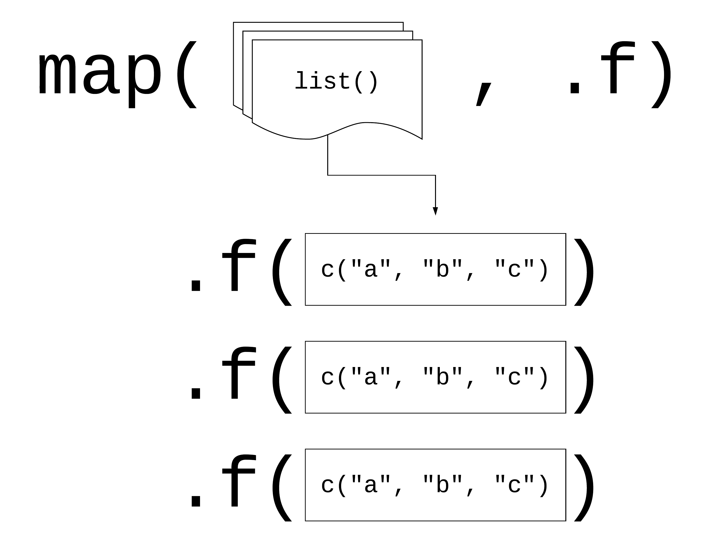
Logic behind vectorised functions (also called functional programming).

Three ways to pass functions to map():

pass directly to map()

map(df, mean, na.rm = TRUE)

use an anonymous function

map(df, function(.x) {
  mean(.x, na.rm = TRUE) }
)

use ~

map(df, ~ mean(.x, na.rm = TRUE))

Let’s look at this in practice. Imagine you want to calculate the mean of each column in your df:

# repetitive code
mean(df$a)
mean(df$b)
mean(df$c)
mean(df$d)


# equivalent map function
map(.x = df, ~ mean(.x, na.rm =T))

# map function in tidyverse style
df %>% map(mean)

The map* family of functions 👪

The pattern of looping over a vector, doing something to each element and saving the results is so common that the purrr package provides a family of functions to do it for you. Indeed, their use is so common that several wrapper functions were created to include the final transformation of the list output. There is one function for each type of output:

map() returns a list.
map_lgl() returns a logical vector
map_int() returns an integer vector.
map_dbl() returns a double vector.
map_chr() returns a character vector.

Exercise 3:

Go back to the example above, since all of the means are numeric, it makes more sense to store them in a vector rather than a list. Which function should I use?

Map2 ‼️

You can also iterate over two inputs at the same time using map2(.x, .y, .f)

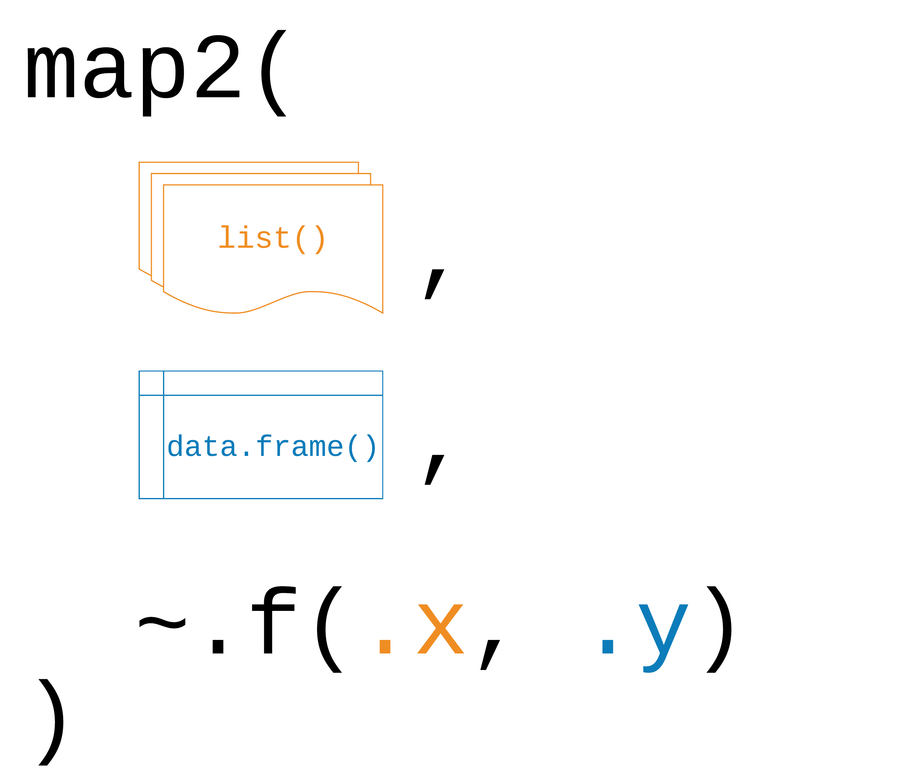
Logic behind map2().

The function works exactly the same way as the map* functions for a single input. One caveat that applies only to map2() is that both inputs need to have the same length!

Exercise 4:

Write a function that returns both the mean and the standard deviation for the numeric variables in our study data.

mean_sd <- function(x) {
  list('mean' = mean(x, na.rm=T), 'sd' = sd(x, na.rm=T))
}

Exercise 5:

Iterate over the relevant columns.

map_df(study %>% select(where(is.numeric)), mean_sd) %>% 
  cbind(
    'col' = study %>% 
      select(where(is.numeric)) %>% 
      colnames()
    )

Exercise 6:

Use map and the tolower function to harmonise character values in the study dataframe.

study %>% select(where(is.character)) %>% map_df(tolower)

Non standard evaluation (optional)

There is, of course, much more to learn about functions in R and for those of you who want to take it further you can find some great resources here or here. For now, consider this as is the first exposure to functions (that can actually already get you pretty far). However, it is important that you apply 🤓 your new skills and practice further on your own.

One such skill is the question of how to integrate tidyverse functions into your own functions. Most dplyr verbs use tidy evaluation in some way. Tidy evaluation is a special type of non-standard evaluation (meaning the way how R interprets your written code) used throughout the tidyverse. There are two basic forms found in dplyr:

data masking makes it so that you can use data variables as if they were variables in the environment (i.e. you write my_variable instead of df$myvariable).
tidy selection allows you to switch choosing variables based on their position, name, or type (e.g. starts_with(“x”) or is.numeric).

Data masking and tidy selection make interactive data exploration fast and fluid, but they add some new challenges when you attempt to use them indirectly such as in a for loop or a function. This vignette shows you how to overcome those challenges.

Debugging 🐞

When you write code, things will inevitably go wrong at some point. You can professionalize the way of how to - fix unanticipated problems (debugging) - let functions communicate problems and take actions based on those communications (condition handling) - learn how to avoid common problems before they occur (defensive programming)

Potential problems are communicated via “conditions”: errors, warnings, and messages. For example - fatal errors are raised by stop() and force all execution to terminate - warnings are generated by warning() and display potential problems - messages are generated by message() and can provide informative output on the way

Debugging workflow

realize that you have a bug
make bug repeatable: start with big block of code and narrow it down to isolate it
figure out where it is
fix it and test it

Debugging tools 🔦

In the lecture, we saw the following function that calculates the geodesic distance between two points specified by radian latitude/longitude using the Haversine formula (hf); taken from here, as an example. We inserted some bugs here… 🐛

# please find the bug fixes in the comments in line

geod_dist <- function(lat1, lon1, lat2, lon2, earth.radius = 6371) {
  # from degrees to radians
  deg2rad <- function(deg) return(deg*pi/180)
  lon1 <- deg2rad(lon1)
  lat1 <- deg2rad(lat1)
  lon2 <- deg2rad(long2) # replace with lon2
  lat2 <- deg2rad(lat2)
  # calculation
  delta.long <- (lon2 - lon1)
  delta.lat <- (lat2 - lat1)
  a <- sin(delta.lat/2)^2 + cos(lat1) * cos(lat2) * sing(delta.long/2)^2 # replace sing with sin
  c <- 2 * asin(min(1,sqrt(a)))
  d = earth_radius * c # replace earth_radius with earth.radius
  return(d)
}

geod_dist(lat1 = 49.5, lon1 = 8.4, lat2 = 52.5, lon2 = 13.4)

Trial and error 🎓

That is, if you see the error right away, try and fix it. You have lots of experience doing that. 🤓

Making function global 🌏

You basically turn the arguments of the function into global objects (objects you can see in your environment, otherwise the objects are only available within your function). Then you can step through the code line by line to locate the bug.

# make the objects that are otherwise entered as input parameters to your function global
lat1 = 49.5; lon1 = 8.4; lat2 = 52.5; lon2 = 13.4

# now, execute line by line
deg2rad <- function(deg) return(deg*pi/180)
lon1 <- deg2rad(lon1)
lat1 <- deg2rad(lat1)
lon2 <- deg2rad(long2)
lat2 <- deg2rad(lat2)
delta.long <- (lon2 - lon1)
delta.lat <- (lat2 - lat1)
a <- sin(delta.lat/2)^2 + cos(lat1) * cos(lat2) * sing(delta.long/2)^2
c <- 2 * asin(min(1,sqrt(a)))
d = earth_radius * c
return(d)

Problem: This creates global objects that match arguments names, which can become confusing and cause problems that become obvious when the function is called in a different environment. ⚠️ In case you choose this option, it is a good idea to clean your environment afterwards, or simply to remove all the new global objects using rm().

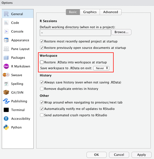
Side note If you haven’t done so already, as a general best practice advise, change the settings in your global options to “never” save the workspace as this can cause similar issues to the example described above.

Using traceback() 👈

geod_dist(lat1 = 49.5, lon1 = 8.4, lat2 = 52.5, lon2 = 13.4)
traceback()

This shows you where the error occurred (but not why). Read from bottom to top (e.g. 1. called function X, 2. called function Y, error occurred in line #6 of function Y)

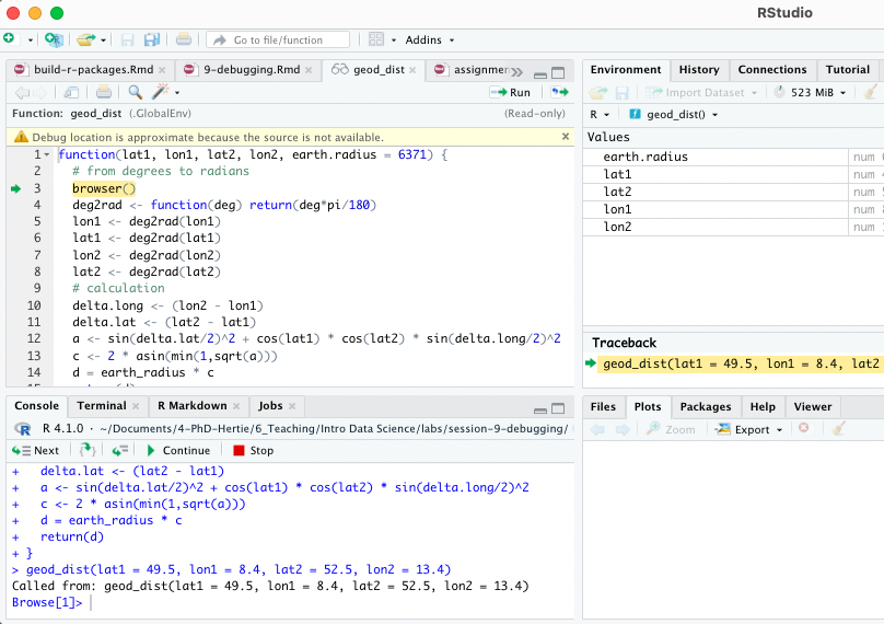
Using browser() 🦊

Basically, add browser() into your function somewhere before you expect the expected error. Note: browser() works best within a clean .R script, it can shoot some troubles within .Rmd.

geod_dist <- function(lat1, lon1, lat2, lon2, earth.radius = 6371) {
  # from degrees to radians
  browser()
  deg2rad <- function(deg) return(deg*pi/180)
  lon1 <- deg2rad(lon1)
  lat1 <- deg2rad(lat1)
  lon2 <- deg2rad(lon2)
  lat2 <- deg2rad(lat2)
  # calculation
  delta.long <- (lon2 - lon1)
  delta.lat <- (lat2 - lat1)
  a <- sin(delta.lat/2)^2 + cos(lat1) * cos(lat2) * sin(delta.long/2)^2
  c <- 2 * asin(min(1,sqrt(a)))
  d = earth_radius * c
  return(d)
}
geod_dist(lat1 = 49.5, lon1 = 8.4, lat2 = 52.5, lon2 = 13.4)

You can then interactively work through the function line by line by hitting enter in the console or send additional lines of code.

Note: Other helpful tools to debug functions in R that you have not written yourself are debug(), that automatically opens a debugger at the start of a function call and trace(), which allows temporary code modifications inside functions that you don’t have easy access to (e.g. ggplot()).

Condition handling 🐜🐜🐝🐜

Sometimes errors come expected, and you want to handle them automatically, e.g.: - model fails to converge - download of files fails - stack processing of lists

Useful functions to deal with such cases: try() and tryCatch()

f1 <- function(x) { 
  log(x) 
  10 
  } 
f1("x")

Using try() 🤷

Ignore error:

f1 <- function(x) { 
  try(log(x))
  10 
} 
f1("x")

## Error in log(x) : non-numeric argument to mathematical function

## [1] 10

Suppress error message:

f1 <- function(x) { 
  try(log(x), silent = TRUE)
  10 
} 
f1("x")

## [1] 10

Pass block of code to try():

try({ 
  a <- 1 
  b <- "x" 
  a + b 
})

## Error in a + b : non-numeric argument to binary operator

Capture the output of try():

success <- try(1 + 2) 
failure <- try("a" + "b")

## Error in "a" + "b" : non-numeric argument to binary operator

class(success)

## [1] "numeric"

class(failure)

## [1] "try-error"

Use possibly(), a function similar to try() from the purrr package when applying a function to multiple elements in a list. You can also provide a default value (here: NA) in case execution fails.

library(purrr)

elements <-list(1,2,3,"f")
results <- map(elements, log)
results <- map(elements, possibly(log, NA))

Condition handling with tryCatch() 🎣

React to conditions, such as errors, warnings, messages, or interruptions, with certain actions “handlers” (functions that are called with the condition as an input) are mapped to condition handler functions can do anything but typically will return a value or create a more informative error message:

show_condition <- function(code) { 
  tryCatch(code, 
           error = function(c) "error", 
           warning = function(c) "warning", 
           message = function(c) "message" )
  }

show_condition(stop("!"))

## [1] "error"

show_condition(warning("?!"))

## [1] "warning"

show_condition(message("?"))

## [1] "message"

If no condition is captured, tryCatch returns the value of the input:

show_condition(10+5)

## [1] 15

A more real-life example of how to use tryCatch() is this one:

model_selection <- function(data, formula1, formula2){

  tryCatch(lm(formula1, data), error = function(e) lm(formula2, data))

}

You try to fit formula1 to the data, however, maybe it is a model with very strict requirements. You might also have a more robust (but maybe less interesting) formula2 that you might fit if the requirements are not met and the modeling process throws an error.

Make more informative error messages

read.csv_new <- function(file, ...) { 
  tryCatch(read.csv(file, ...), error = function(c) {
    c$message <- paste0(c$message, " (in ", file, ")") 
    stop(c) 
  })
}

read.csv("code/dummy.csv")
read.csv_new("code/dummy.csv")

Defensive programming 🛡

“making code fail in a well-defined manner”
“fail fast”: as soon as something wrong is discovered, signal an error
Three rules to implement the “fail fast” principle:

be strict about what you accept (e.g., only scalars)
avoid functions that use non-standard evaluation, such as subset(), transform(), or with()
avoid functions that return different types of output depending on their input, e.g. [ and sapply

Debugging Exercise 💀

Here is a piece of code that comes with quite some flaws. As an optional take-home exercise, please identify the bugs, remove them and report what you have done using comments.

# load packages
library(tidyverse)
library(LegislatoR) # legislatoR

# get political data on German legislators
political_df <- 
  left_join(x = filter(get_political(legislature = "ger"), as.numeric("session") == 18), # issue with the filter and retrieval, see solution
            y = get_core(legislature = "ger"), by = "pageid") # deu instead of ger

# wiki traffic data
traffic_df <- 
  get_traffic(legislature = "ger") %>% # deu instead of ger
  filter(date >= "2013-10-22" & date <= "2017-10-24") %>% 
  group_by(pageid) %>% 
  summarize(traffic_mean = mean(traffic, na.rm = TRUE),
            traffic_max = max(traffic, na.rm = TRUE))

# sessions served
sessions_served_df <- 
  get_political(legislature = "deu") %% # error in the pipe
  group_by(pageid) %>% 
  dplyr::summarize(sessions_served = n())

# merge
legislator_df <- 
  left_join(political_df, sessions_served_df, by = "pageid") %>% 
  left_join(traffic_df, by = "pageid") 

# compute age
get_age <- function(birth, date_at) {
  date_at_fmt <- date_at
  birth_fmt <- birth
  diff <- difftime(lubridate::ymd(birth_fmt), lubridate::ymd(date_at_fmt)) # switch death and birth
  diff_years <- time_length(diff, "years") # you need load the lubridate function here
  diff_years
}
legislator_df$age_in_years <- round(get_age(legislator_df$birth, "2017-10-24"), 0)

# plot top 10 pageviews
legislator_df <- arrange(legislator_df, desc(traffic_mean))
legislator_df$rank <- 1:nrow(legislator_df)
legislator_df_table <- dplyr::select(rank, name, traffic_mean, traffic_max) # pass the dataframe
names(legislator_df_table) <- c("Rank", "Representative", "Mean", "Maximum") # change to colnames()
legislator_df_table <- head(legislator_df_table, 10)

ggplot(legislator_df_table, aes(y = Mean, x = -Rank)) + 
  xlab("Rank") + ylab("Avg. daily page views") + 
  labs(title = "Top 10 representatives by average daily page views") + 
  geom_bar(stats = "identity") + # change to geom_col
  scale_x_continuous(breaks = -nrow(legislator_df_table):-1, labels = rev(1:nrow(legislator_df_table))) # add +
  geom_text(aes(y = 10, label = Representative), hjust = 0, color = "white", size = 2) + 
  coord_flip() + 
  theme_minimal()

# run model of page views as a function of sessions served, party, sex, and age in years
legislator_df$traffic_log <- log(legislator_df$traffic_mean)

covars <- c("sessions_served", "party", "sex", "age_in_years")
fmla <- paste("traffic_log", paste(covars, collapse = " - "), sep = " ~ ") # collapse with +
summary(log_traffic_model <- lm(fmla, legislator_df))

# plot table
sjPlot::tab_model(log_traffic_model)

Actually learning R 🎒

Let us remind you again, the key to learning R is: Google! We can only give you an overview over basic R functions, but to really learn R you will have to actively use it yourself, trouble shoot, ask questions, and google! It is very likely that someone else has had the exact same or just similar enough issue before and that the R community has answered it with 5+ different solutions years ago. 😉

Sources

The section on functions and iteration is partly based on R for Data Science, section 5.2, Quantitative Politics with R, chapter 3; as well as the Tidyverse Session and on the excellent slides by Malcolm Barrett in the course Data Science for Economists by Grant McDermott. The data for the exercises was inspired by R for Epidemiology. The section on functions relies

A work by Lisa Oswald & Tom Arend

Prepared for Intro to Data Science, taught by Simon Munzert

Hertie School, Berlin

Functional Programming

Functions, iteration and debugging in R

Quick review: lists 📃

Functions 🏭

Basic Syntax

Exercise 1:

Exercise 2:

Conditional functions 🔀

Exercise 3:

Iteration ⚙️

For-loops

While-loops

The `purrr` package 🐱

Basic syntax 🖊

The map* family of functions 👪

Exercise 3:

Map2 ‼️

Exercise 4:

Exercise 5:

Exercise 6:

Non standard evaluation (optional)

Debugging 🐞

Debugging workflow

Debugging tools 🔦

Trial and error 🎓

Making function global 🌏

Using traceback() 👈

Using browser() 🦊

Condition handling 🐜🐜🐝🐜

Using try() 🤷

Condition handling with tryCatch() 🎣

Defensive programming 🛡

Debugging Exercise 💀

Actually learning R 🎒

Sources

Functional Programming

Functions, iteration and debugging in R

Quick review: lists 📃

Functions 🏭

Basic Syntax

Exercise 1:

Exercise 2:

Conditional functions 🔀

Exercise 3:

Iteration ⚙️

For-loops

While-loops

The purrr package 🐱

Basic syntax 🖊

The map* family of functions 👪

Exercise 3:

Map2 ‼️

Exercise 4:

Exercise 5:

Exercise 6:

Non standard evaluation (optional)

Debugging 🐞

Debugging workflow

Debugging tools 🔦

Trial and error 🎓

Making function global 🌏

Using traceback() 👈

Using browser() 🦊

Condition handling 🐜🐜🐝🐜

Using try() 🤷

Condition handling with tryCatch() 🎣

Defensive programming 🛡

Debugging Exercise 💀

Actually learning R 🎒

Sources

The `purrr` package 🐱