Web Scraping
Collecting Data from the Web using R
After talking quite a bit about data formats and data processing in the past weeks, today’s session is dedicated to data collection - from the web!
What we will cover:
- basic web technologies (html, xpath)
- scraping static webpages
- scraping multiple static webpages
- building up and maintaining you own original sets of web-based data
What we will not cover (today):
- scraping dynamic webpages
- APIs
- extensive data cleaning using regular expressions
Why webscrape with R? 🌐
Webscraping broadly includes a) getting (unstructured) data from the web and b) bringing it into shape (e.g. cleaning it, getting it into tabular format).
Why webscrape? While some influential people consider “Data Scientist” 👩💻 as the sexiest job of the 21st century (congratulations!), one of the sexiest just emerging academic disciplines (my influential view) - Computational Social Science (CSS). Why so?
- data abundance online
- social interaction online
- services track social behavior
BUT online data are usually meant for display, not (clean) download!
But getting access to online data would also be incredibly interesting when you think of very pragmatic things like financial resources, time resources, reproducibility and updateability…
Luckily, with R we can automate the whole pipeline of downloading, parsing and post-processing to make our projects easily reproducible.
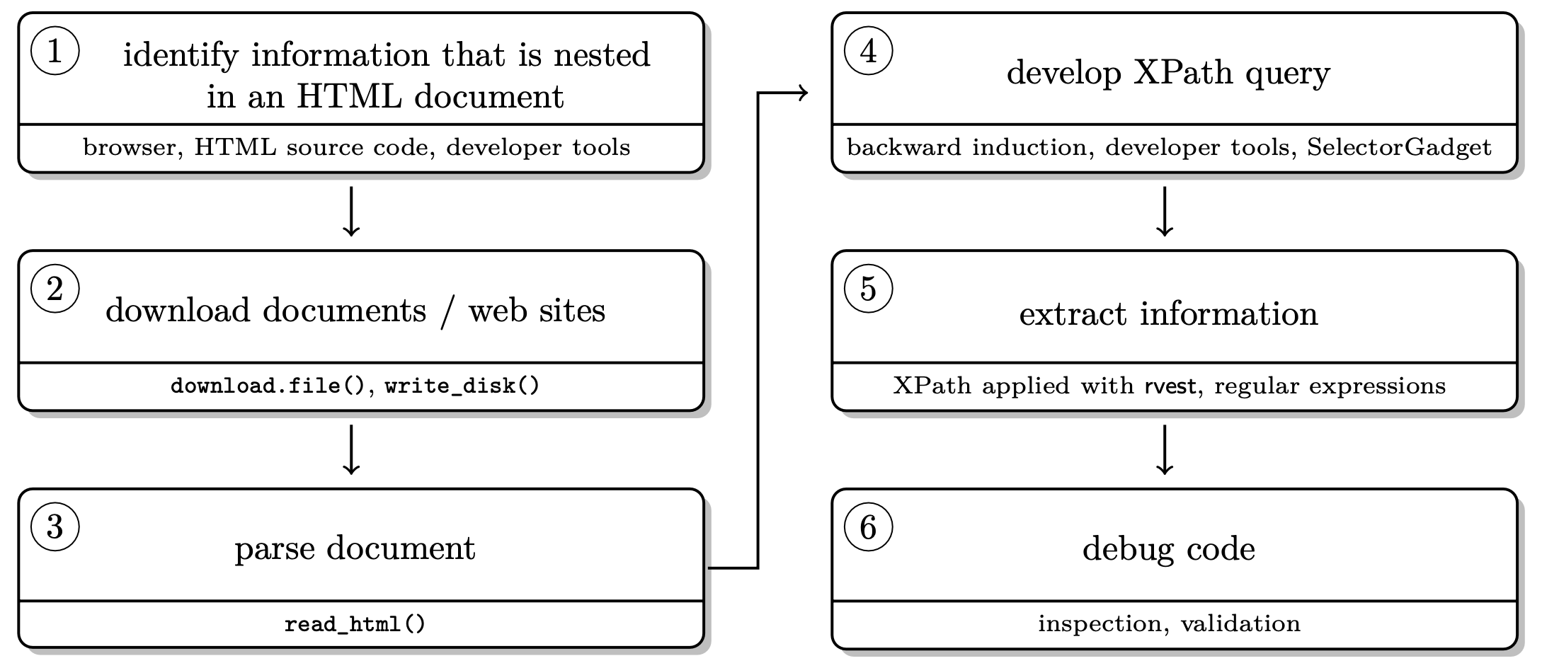
In general, remember, the basic workflow for scraping static webpages is the following.
Scraping static websites with rvest 🚜
Who doesn’t love Wikipedia? Let’s use this as our first, straight forward test case.
Step 1. Load the packages rvest and stringr.
library(rvest)
library(stringr)
Step 2. Parse the page source.
parsed_url <- read_html("https://en.wikipedia.org/wiki/Cologne")Step 3. Extract information.
parsed_nodes <- html_nodes(parsed_url,
                           xpath = '//p[(((count(preceding-sibling::*) + 1) = 157) and parent::*)]')
carnival <- html_text(parsed_nodes)
carnival
## [1] "Cologne is also famous for Eau de Cologne (German: Kölnisch Wasser; lit: \"Water of Cologne\"), a perfume created by Italian expatriate Johann Maria Farina at the beginning of the 18th century. During the 18th century, this perfume became increasingly popular, was exported all over Europe by the Farina family and Farina became a household name for Eau de Cologne. In 1803 Wilhelm Mülhens entered into a contract with an unrelated person from Italy named Carlo Francesco Farina who granted him the right to use his family name and Mühlens opened a small factory at Cologne's Glockengasse. In later years, and after various court battles, his grandson Ferdinand Mülhens was forced to abandon the name Farina for the company and their product. He decided to use the house number given to the factory at Glockengasse during the French occupation in the early 19th century, 4711. Today, original Eau de Cologne is still produced in Cologne by both the Farina family, currently in the eighth generation, and by Mäurer & Wirtz who bought the 4711 brand in 2006.\n"How can do I know THIS xpath = '//p[(((count(preceding-sibling::*) + 1) = 157) and parent::*)]' ?
There are two options:
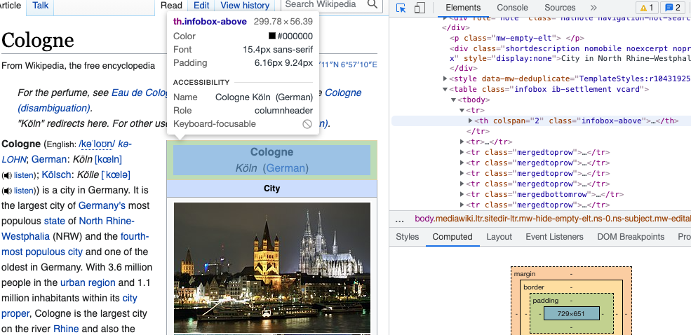
Option 1. On your page of interest, go to a table that you’d like to scrape. Our favorite bowser for webscraping is Google Chrome but others work as well. On Chrome, you go in View > Developer > inspect elements. If you hover over the html code on the right, you should see boxes of different colors framing different elements of the page. Once the part of the page you would like to scrape is selected, right click on the html code and Copy > Copy Xpath. That’s it.
Option 2. You download the Chrome Extension SelectorGadget and activate it while browsing the page you’d like to scrape from. You will see a selection box moving with your cursor. You select an element by clickin on it. It turns green - and so does all other content that would be selected with the current XPath.
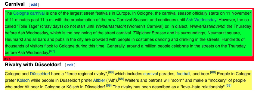
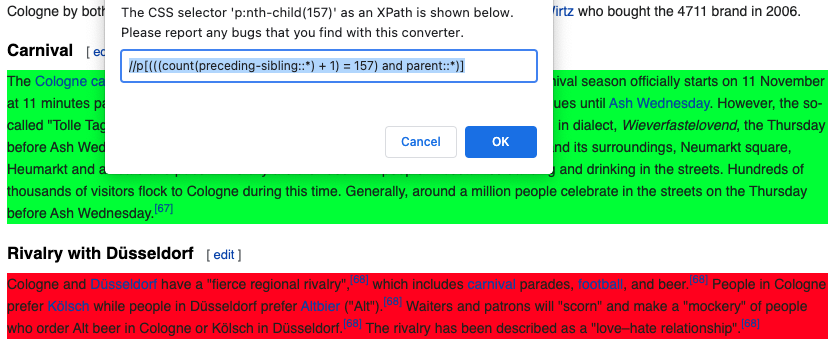
You can now de-select everything that is irrelevant to you by clicking it again (it then turns red). Final step, then just click the XPath button at the bottom of the browser window. Make sure to use single quotation marks with this XPath!
Let’s repeat step 2 and 3 with a more data-sciency example. 🕺
Step 2. Parse the page source.
hot100page <- "https://www.billboard.com/charts/hot-100"
hot100 <- read_html(hot100page)
Step 3. Extract information. When going through different levels of html, you can also use tidyverse logic.
body_nodes <- hot100 %>%
 html_node("body") %>%
 html_children()

body_nodes %>%
 html_children()
play with that yourself if you like…
Now let’s get more specific - xml_find_all() takes xpath syntax!
rank <- hot100 %>%
  rvest::html_nodes('body') %>%
  xml2::xml_find_all("//span[contains(@class, 'chart-element__rank__number')]") %>%
  rvest::html_text()

artist <- hot100 %>%
  rvest::html_nodes('body') %>%
  xml2::xml_find_all("//span[contains(@class, 'chart-element__information__artist')]") %>%
  rvest::html_text()

title <- hot100 %>%
  rvest::html_nodes('body') %>%
  xml2::xml_find_all("//span[contains(@class, 'chart-element__information__song')]") %>%
  rvest::html_text()
Step 4. Usually, step 4 is to clean extracted data. In this case, it actually is very clean already. However, if you need help with data cleaning using regular expressions (me, always.), visit the section of R for Data Science or simply this cheat sheet.
Step 5. Put everything into a data frame. 🎵
chart_df <- data.frame(rank, artist, title)

knitr::kable(chart_df %>% head(10))| rank | artist | title |
|---|---|---|
| 1 | Lil Nas X & Jack Harlow | Industry Baby |
| 2 | The Kid LAROI & Justin Bieber | Stay |
| 3 | Walker Hayes | Fancy Like |
| 4 | Ed Sheeran | Bad Habits |
| 5 | Drake Featuring Future & Young Thug | Way 2 Sexy |
| 6 | Olivia Rodrigo | Good 4 U |
| 7 | Doja Cat Featuring SZA | Kiss Me More |
| 8 | Dua Lipa | Levitating |
| 9 | Wizkid Featuring Justin Bieber & Tems | Essence |
| 10 | Ed Sheeran | Shivers |
Scraping HTML tables 🚀
We have just been scraping an html table… but there is even an easier way to do this in rvest!
url_p <- read_html("https://en.wikipedia.org/wiki/List_of_human_spaceflights")
tables <- html_table(url_p, header = TRUE, fill = TRUE)
spaceflights <- tables[[1]]

knitr::kable(spaceflights[,1:7] %>% head(10))| Entity | Soviet Union | Soviet Union | Soviet Union | United States | United States | United States |
|---|---|---|---|---|---|---|
| Agency | Soviet space program | Soviet space program | Soviet space program | NASA | NASA | NASA |
| Decades | Program | Dates[a] | No.[b] | Program[c] | Dates | No.[d] |
| 1961–1970 | Vostok | 1961–1963 | 6 | Mercury | 1961–1963 | 6 |
| 1961–1970 | Voskhod | 1964–1965 | 2 | X-15 | 1962–1968 | 13 |
| 1961–1970 | Soyuz | 1967–1991 | 63 | Gemini | 1965–1966 | 10 |
| 1961–1970 | Soyuz | 1967–1991 | 63 | Apollo | 1968–1972 | 11 |
| 1971–1980 | Soyuz | 1967–1991 | 63 | Apollo | 1968–1972 | 11 |
| 1971–1980 | Soyuz | 1967–1991 | 63 | Skylab | 1973–1974 | 3 |
| 1971–1980 | Soyuz | 1967–1991 | 63 | Apollo–Soyuz | 1975 | 1 |
| 1981–1990 | Soyuz | 1967–1991 | 63 | Space Shuttle | 1981–2011 | 135 |
Another R workaround for more complex tables is the package htmltab that offers some more flexibility.
It’s your turn! 🛠
Think about web data hosted on a static webpage that you might be interested in scraping! Comparably easy to scrape webpages are Wikipedia pages or pages that contain data in table format (as we’ve seen already).
Before you start - it might be worth a thought to get Chrome + Selector Gadget. This will make your future as web scraper a bit easier.
Option A
Inspect the page and try to find the elements you are interested in in the html code.
Parse the url.
Extract the XPath for the element you would like to scrape and parse the nodes.
Inspect the html output you get. What would be the next steps now? Can you already put your output into a dataframe?
Option B
Find an html table that you’d like to scrape.
Scrape it.
Scraping multiple pages 🤖
Whenever you want to really understand what’s going on within the functions of a new R package, it is very likely that there is a relevant article published in the Journal of Statistical Software. Let’s say you are interested in how the journal was doing over the past years.
Step 1. Inspect the source. Basically, follow steps to extract the Xpath information.
browseURL("http://www.jstatsoft.org/issue/archive")Step 2 Develop a scraping strategy. We need a set of URLs leading to all sources. Inspect the URLs of different sources and find the pattern. Then, construct the list of URLs from scratch.
baseurl <- "http://www.jstatsoft.org/article/view/v"
volurl <- paste0("0", seq(1, 99, 1))
volurl[1:9] <- paste0("00", seq(1, 9, 1))
brurl <- paste0("0", seq(1, 9, 1))
urls_list <- paste0(baseurl, volurl)
urls_list <- paste0(rep(urls_list, each = 9), "i", brurl)
urls_list[1:5]
## [1] "http://www.jstatsoft.org/article/view/v001i01"
## [2] "http://www.jstatsoft.org/article/view/v001i02"
## [3] "http://www.jstatsoft.org/article/view/v001i03"
## [4] "http://www.jstatsoft.org/article/view/v001i04"
## [5] "http://www.jstatsoft.org/article/view/v001i05"Step 3 Think about where you want your scraped material to be stored and create a directory.
tempwd <- ("data/jstatsoftStats")
dir.create(tempwd)
setwd(tempwd)
Step 4 Download the pages. Note that we did not do this step last time, when we were only scraping one page.
folder <- "html_articles/"
dir.create(folder)

for (i in 1:length(urls_list)) {
  # only update, don't replace
    if (!file.exists(paste0(folder, names[i]))) {
  # skip article when we run into an error
      tryCatch(
        download.file(urls_list[i], destfile = paste0(folder, names[i])),
        error = function(e) e
      )
  # don't kill their server --> be polite!
      Sys.sleep(runif(1, 0, 1))

} }
While R is downloading the pages for you, you can watch it directly in the directory you defined…
Check whether it worked.
list_files <- list.files(folder, pattern = "0.*")
list_files_path <- list.files(folder, pattern = "0.*", full.names = TRUE)
length(list_files)
Yay! Apparently, we scraped the html pages of 802 articles.
(Git)ignoring files 🙅
In case you scraping project is is linked to GitHub (as it will be in your assignment!), it can be useful to .gitignore the folder of downloaded files. This means that the folder can be stored in your local directory of the project but will not be synced with the remote (main) repository. Here is information on how to do this using RStudio. In Github Desktop it is very simple, you do your scraping work, the folder is created in your local repository and before your commit and push these changes, you go on Repository > Repository Settings > Ignored Files and edit the .gitignore file (add the name of the new folder / files you don’t want to sync). More generally, it makes sense to exclude .Rproj files, .RData files (and other binary or large data files), draft folders and sensitive information from version control. Remember, git is built to track changes in code, not in large data files.
Step 5 Import files and parse out information. A loop is helpful here!
# define output first
authors <- character()
title <- character()
datePublish <- character()

# then run the loop
for (i in 1:length(list_files_path)) {
  html_out <- read_html(list_files_path[i])

  authors[i] <- html_text(html_nodes(html_out , xpath = '//*[contains(concat( " ", @class, " " ), concat( " ", "authors_long", " " ))]//strong'))

  title[i] <- html_text(html_nodes(html_out , xpath = '//*[contains(concat( " ", @class, " " ), concat( " ", "page-header", " " ))]'))

  datePublish[i] <- html_text(html_nodes(html_out , xpath = '//*[contains(concat( " ", @class, " " ), concat( " ", "article-meta", " " ))]//*[contains(concat( " ", @class, " " ), concat( " ", "row", " " )) and (((count(preceding-sibling::*) + 1) = 2) and parent::*)]//*[contains(concat( " ", @class, " " ), concat( " ", "col-sm-8", " " ))]'))
}

# inspect data
authors[1:3]
title[1:2]
datePublish[1:3]

# create a data frame
dat <- data.frame(authors = authors, title = title, datePublish = datePublish)
dim(dat)
Step 6 Clean data…
You see, scraping data from multiple pages is no problem in R. Most of the brain work often goes into developing a scraping strategy and tidying the data, not into the actual downloading/scraping part.
Scraping is also possible in much more complex scenarios! Watch out for workshop presentations on
- Dynamic webscraping with RSelenium
- Web APIs
- Regular expressions with stringr
- Data cleaning with janitor
and many more 🤩
Good scraping practice
There is a set of general rules to the game:
- You take all the responsibility for your web scraping work.
- Think about the nature of the data. Does it entail sensitive information? Do not collect personal data without explicit permission.
- Take all copyrights of a country’s jurisdiction into account. If you publish data, do not commit copyright fraud.
- If possible, stay identifiable. Stay polite. Stay friendly. Obey the scraping etiquette.
- If in doubt, ask the author/creator/provider of data for permission—if your interest is entirely scientific, chances aren’t bad that you get data.
How do I know the scraping etiquette of a site? 🤝
Robot exclusion standards (robot.txt) are informal protocols to prohibit web robots from crawling content. They list documents that are allowed to crawl and which not. It is not a technical barrier but an ask for compliance. They are located in the root directory of a website (e.g https://de.wikipedia.org/robots.txt).
For example, let’s have a look at wikipedia’s robot.txt file, which is very human readable.
General rules are listed under User-agent: * which is most interesting for R-based crawlers. A universal ban for a directory looks like this Disallows: /, sometimes Crawl-delays are suggested (in seconds) Crawl-delay: 2.
What is “polite” scraping? 🐌
First thing would be not to scrape at a speed that causes trouble for their server. Therefore, whenever you loop over a list of URLs, add a Sys.sleep(runif(1, 1, 2)) at the end of the loop.
And generally, it is better practice to store data on your local drive first (download.file()), then parse (read_html()).
A footnote on sustainability. In the digital context, we often forget that or actions do have physical consequences. For example, training AI, using blockchain and just streaming videos do cause considerable amounts of CO2 emissions. So does bombarding a server with requests - certainly to a much lesser extent than the examples before - but please consider whether you have to re-run a large scraping project 100 times in order to debug things.
Furthermore, downloading massive amounts of data may arouse attention from server administrators. Assuming that you’ve got nothing to hide, you should stay identifiable beyond your IP address.
How can I stay identifyable? 👤
Option 1: Get in touch with website administrators / data owners.
Option 2: Use HTTP header fields From and User-Agent to provide information about yourself.
url <- "http://a-totally-random-website.com"

rvest_session <- session(url,
  add_headers(`From` = "my@email.com",
              `UserAgent` = R.Version()$version.string))

scraped_text <- rvest_session %>%
            html_elements(xpath = "p//a") %>%
            html_text()
rvest’s session() creates a session object that responds to HTTP and HTML methods. Here, we provide our email address and the current R version as User-Agent information. This will pop up in the server logs: The webpage administrator has the chance to easily get in touch with you.
Sources
This tutorial drew heavily on Simon Munzert’s book Automated Data Collection with R and related course materials. We also used an example from Keith McNulty’s blog post on tidy web scraping in R.
A work by Lisa Oswald & Tom Arend
Prepared for Intro to Data Science, taught by Simon Munzert