Introduction

Many “big data” problems are actually “small data problems in disguise”. That is, we only really need a subset of the data, or maybe we want to aggregate the data into some larger dataset. For example, we might want to access Census data, but only for a handful of municipalities. Or, we might want to analyse climate data collected from a large number of weather stations, but aggregated up to the national or monthly level. In such cases, the underlying bottleneck is interacting with the original data, which is too big to fit into memory. How do we store data of this magnitude and and then access it effectively? The answer is through a database.

Databases can exist either locally or remotely, as well as in-memory or on-disk. Regardless of where a database is located, the key point is that information is stored in a way that allows for very quick extraction and/or aggregation. More oftne than not you will probably need to extract several subsets and harmonise or transform them. To facilitate and automate this task, you will need to write your own functions and know to iterate them over the relevant subsets of data. This week’s session thus ties in well with the sections on functions and iteration that we quickly touched upon during the last lab.

Functions and Databases 🔭

Although this week’s session is nominally about databases - and we will spend a substantial part of this session on them - we believe that writing your own functions is a key skill that deserves more attention than we were able to devote to it during last week’s session. Therefore, we will split the session in two. First we will cover functions and iterations. In that section you will learn to:

write your own functions (a key skill for all R users)
iterate functions over multiple inputs

The second part of the session will deal with databases and SQL. Here you will learn to:

connect to remote databases with R
generate SQL queries in R with dbplyr
manipulate and transform data in a remote database
how to collect hosted data and store it locally

Functions

In any coding language a fundamental principle should be DRY (Don’t Repeat Yourself). You should adhere to this as much as possible. Functions are the perfec tool for this.

Functions allow you to automate tasks in a more powerful and general way than copy-and-pasting. Writing a function has three big advantages over using copy-and-paste:

You can give a function an evocative name that makes your code easier to understand.
As requirements change, you only need to update code in one place, instead of many.
You eliminate the chance of making incidental mistakes when you copy and paste (i.e. updating a variable name in one place, but not in another).

You can read more on functions in this section of R for Data Science.

Generally, how does code look like that calls for writing a function? For example like this:

df <- data.frame(
  a = rnorm(100, 5, 2),
  b = rnorm(100, 100, 15),
  c = rnorm(100, 2, 1),
  d = rnorm(100, 36, 7)
)

df$a <- (df$a - mean(df$a, na.rm = TRUE)) / sd(df$a, na.rm = TRUE)
df$b <- (df$b - mean(df$b, na.rm = TRUE)) / sd(df$a, na.rm = TRUE) # spot the mistake?
df$c <- (df$c - mean(df$c, na.rm = TRUE)) / sd(df$c, na.rm = TRUE)
df$d <- (df$d - mean(df$d, na.rm = TRUE)) / sd(df$d, na.rm = TRUE)

There are three key steps to creating a new function:

Pick a name for the function. For us it could be zscale because this function rescales (or z-transforms) a vector to have a mean of 0 and a standard deviation of 1.
You list the inputs, or arguments, to the function inside function. Here we have just one argument. If we had more the call would look like function(x, y, z).
You place the code you have developed in body of the function, a { block that immediately follows function(…).

The overall structure of a function looks like this in R:

function_name <- function(input_parameters){
  Do what you want to do in the body of the
  function, just like you would write other code in R.
}

In our example, we could simplify the z-transformation of 4 variables with this function:

zscale <- function(x){
  (x - mean(x, na.rm = T) / sd(x, na.rm = T))
}

A word on function names. Generally, function names should be verbs, and arguments should be nouns. There are some exceptions: nouns are ok if the function computes a very well known noun (i.e. mean), or accessing some property of an object (i.e. coefficients). A good sign that a noun might be a better choice is if you’re using a very broad verb like “get”, “compute”, “calculate”, or “determine”. Where possible, avoid overriding existing functions and variables. However, many good names are already taken by other packages, but avoiding the most common names from base R will avoid confusion.

Conditions

You can of course also add conditions to your function.

if (this) {
  # do that
} else if (that) {
  # do something else
} else {
  # 
}

You could, for example, only transform numeric variables.

zscale <- function(x){
  if (is.numeric(x)) {
  (x - mean(x, na.rm = T) / sd(x, na.rm = T))
  }
}

We can now apply our function to any variable that we would like to transform.

df$a <- zscale(df$a)
df$b <- zscale(df$b)
df$c <- zscale(df$c)
df$d <- zscale(df$d)

# you can also use your function with a pipe!
df$d %>% zscale()

Note that there is still a lot of repetition. We can get rid of this using iteration 👇

Iteration

Iteration helps you when you need to do the same thing to multiple inputs: repeating the same operation on different columns, or on different datasets.

On the one hand, you have for loops and while loops which are a great place to start because they make iteration very explicit. On the other hand, functional programming (FP) offers tools to extract out duplicated code, so each common for loop pattern gets its own function.

Remember the code above - it violates the rule of thumb that you should not copy and paste more than twice.

# repetitive code
df$a <- zscale(df$a)
df$b <- zscale(df$b)
df$c <- zscale(df$c)
df$d <- zscale(df$d)

# equivalent iteration
for (i in seq_along(df)) {       # seq_along() similar to length()
  df[[i]] <- zscale(df[[i]])     # [[]] because we are working on single elements
}

To solve problems like this one with a for loop we again think about the three components:

Output: we already have the output — it’s the same as the input because we are modifying data. If that is not the case, make sure to define a space where the output should go (e.g. an empty vector). If the length of your vector is unknown, you might be tempted to solve this problem by progressively growing the vector. However, this is not very efficient because in each iteration, R has to copy all the data from the previous iterations. In technical terms you get “quadratic” (O(n^2)) behaviour which means that a loop with three times as many elements would take nine (3^2) times as long to run. A better solution to save the results in a list, and then combine into a single vector after the loop is done. See more on this here.
Sequence: we can think about a data frame as a list of columns, so we can iterate over each column with seq_along(df).
Body: apply zscale() or any other function.

Functionals 🐱

For loops are not as important in R as they are in other languages because R is a functional programming language. This means that it’s possible to wrap up for loops in a function, and call that function instead of using the for loop directly. 💡

The purrr package provides functions that eliminate the need for many common for loops. The apply family of functions in base R (apply(), lapply(), tapply(), etc.) solve a similar problem, but purrr is more consistent and thus is easier to learn.

The pattern of looping over a vector, doing something to each element and saving the results is so common that the purrr package provides a family of functions to do it for you. There is one function for each type of output:

map() makes a list.
map_lgl() makes a logical vector.
map_int() makes an integer vector.
map_dbl() makes a double vector.
map_chr() makes a character vector.

Each function takes a vector as input, applies a function to each piece, and then returns a new vector that’s the same length (and has the same names) as the input. The type of the vector is determined by the suffix to the map function.

Let’s look at this in practice. Imagine you want to calculate the mean of each column in your df:

# repetitive code
mean(df$a)
mean(df$b)
mean(df$c)
mean(df$d)

# equivalent map function
map_dbl(df,mean)

# map function in tidyverse style
df %>% map_dbl(mean)

There is, of course, much more to learn about functions in R and we could dedicate an entire session to it. For now, consider this as is the first exposure to functions (that can actually already get you pretty far). However, it is important that you apply 🤓 you new skills and practice further on your own. A good starting point is obviously assignment 2 that is due tonight!!!. Good luck! 🤞

Exercises (Part I)

For the following exercises let’s load a fictional experimental study dataset “study.csv” that was generated for this course.

library(tidyverse)
study <- read_csv("./study.csv")

glimpse(study)

## Rows: 68
## Columns: 8
## $ age       <dbl> 32, 30, 32, 29, 24, 38, 25, 24, 48, 29, 22, 29, 24, 28, 24, …
## $ age_group <chr> "30 and Older", "30 and Older", "30 and Older", "Younger tha…
## $ gender    <chr> "Male", "Female", "Female", "Male", "Female", "Female", "Fem…
## $ ht_in     <dbl> 70, 63, 62, 67, 67, 58, 64, 69, 65, 68, 63, 68, 69, 66, 67, …
## $ wt_lbs    <dbl> 216, 106, 145, 195, 143, 125, 138, 140, 158, 167, 145, 297, …
## $ bmi       <dbl> 30.99, 18.78, 26.52, 30.54, 22.39, 26.12, 23.69, 20.67, 26.2…
## $ bmi_3cat  <chr> "Obese", "Normal", "Overweight", "Obese", "Normal", "Overwei…
## $ emotions  <chr> "sad", "netural", "netural", "netural", "happy", "sad", "net…

You feel that the variable on emotions is badly represented in the data and you decide to replace it with Emoticons! You want to write a function to automate this task. Transform this pseudo code into an R function:

replace_w_emoticons <- # If person is "happy", person is ":)", 
                       # Else if person is emotion "neutral", person is ":/"
                       # Else person is ":("

Create a new column in the dataset that contains these Smiles.
You are also interested in getting some descriptive statistics, notably for age, height and weight. Since this is but a sample of the overall population you should use inference and calculate the mean with a Confidence Interval around it. Here is a function that does it, but we only get NAs. How do we fix this function?

mean_ci <- function(x, conf = 0.95) {
  se <- sd(x) / sqrt(length(x)) 
  alpha <- 1 - conf
  mean(x) + se * qnorm(c(alpha / 2, 1 - alpha / 2))
}

mean_ci(study$age)

## [1] NA NA

Now that we fixed the function, how can we apply it to the different variables? Rewrite this chunk of code so that we do not repeat ourselves:

mean_ci(study$age)
mean_ci(study$ht_in)
mean_ci(study$wt_lbs)

For more practice with functions have a look at the following practice script.

Working with databases 💾

So far, we have dealt with small datasets that easily fit into your computer’s memory. But what about datasets that are too large for your computer to handle as a whole? In this case, storing the data outside of R and organizing it in a database is helpful. Connecting to the database allows you to retrieve only the parts needed for your current analysis.

Even better, many large datasets are already available in public or private databases. You can query them without having to download the data first.

Necessary packages

Accessing databases in R requires a few packages:

dbplyrmakes use of the same functions as dplyr, but also works with remote data stored in databases.
DBI is a package that allows R to connect easily to a DBMS (DataBase Management System)
Some package to interact with the back-end of the remote database such as RSQLite, other options might be:
RMariaDB::MariaDB() for RMariaDB,
RPostgres::Postgres() for RPostgres,
odbc::odbc() for odbc,
and bigrquery::bigquery() for BigQuery.

Connecting to a database

To connect to the database, we will use dbConnect() from the DBI package which defines a common interface between R and database management systems. The first argument is the database driver which in our case is SQLite and the second argument is the name and location of the database.

Most existing databases don’t live in a file, but instead live on another server. In addition to the two arguments above, database drivers will therefore also require details like user, password, host, port, etc. That means your code will often look more like this:

con <- DBI::dbConnect(RMariaDB::MariaDB(), 
                      host = "database.rstudio.com",
                      user = "tom",
                      password = rstudioapi::askForPassword("Tom's password")
)

For the purposes of this lab however, we are connecting to an in-memory database. That way we can avoid potential issues regarding the registration for access to a database, creation and caching of credentials, as well as defining safe ports and other boring details.

To avoid all this hassle, we basically create and host our own (small) database. Luckily, the code to do so is the same as in the general case above. But, SQLite only needs a path to the database. (Here, “:memory:” is a special path that creates an in-memory database.)

We then save the database connection and store it in the object “con” for further use in exploring and querying data.

# set up connection with DBI and RSQLite
con <- dbConnect(RSQLite::SQLite(), ":memory:")

Next, let us get a quick summary of the database connection using summary(). It shows “SQLiteConnection” under class and we can ignore the other details for the time being. Great!

summary(con)

##           Length            Class             Mode 
##                1 SQLiteConnection               S4

If you were to connect to a real online database that someone else generated, you could now call DBI::dbListTables(con) to see a list of the tables present in the database. Our local database is however still devoid of content.

We need to populate our database. We copy the data from last week to our database connection. In real life this step would probably be taken care of by the responsible database maintainer.

# upload local data frame into remote data source; here: database
copy_to(
  dest = con, 
  df = nycflights13::flights, 
  name = "flights")

Indexing

Unfortunately, it is not enough to just copy data to our database. We also need to pass a list of indexes to the function. In this example, we set up indexes that will allow us to quickly process the data by time, carrier, plane, and destination. Creating the right indices is key to good database performance. Again, in applications where we don’t set up the database, this will be taken care of by the database maintainer.

copy_to(
  dest = con, 
  df = nycflights13::flights, 
  name = "flights",
  temporary = FALSE, 
  indexes = list(
    c("year", "month", "day"), 
    "carrier", 
    "tailnum",
    "dest"
  ),
  overwrite = T # throws error as table already exists
)

List Tables in Database

Now that we are connected to a database, let us list all the tables present in it using dbListTables().

DBI::dbListTables(con)

## [1] "flights"      "sqlite_stat1" "sqlite_stat1" "sqlite_stat4" "sqlite_stat4"

As you can see there is only one table for now (flights). The other objects that show up are infrastructure specificities for SQLite that you can safely ignore. Usually you would find many different tables in a relational database.

Queries

A query is a request for data or information from a database table or combination of tables. 📖

Reference Table

So how do you query a table in a database?

It is actually fairly straightforward. You use the tbl()function where you indicate the connection and the name of the table you want to interact with.

# generate reference table from the database
flights_db <- tbl(con, "flights")
flights_db

The console output shows that this is a remote source; the table is not stored in our RStudio environment. Nor should you need to transfer the entire table to your RStudio environment. You can perform operations directly on the remote source. What is more you can rely on the dplyr syntax from last week to formulate your queries. R will automatically translate it into SQL (more on that below).

Selecting Columns

You can select specific columns:

# perform various queries
flights_db %>% select(year:day, dep_delay, arr_delay)

Filtering by Rows

Access only specific rows:

flights_db %>% filter(dep_delay > 240)

Summary Statisitics

Or immediately generate summary statistics for different groups:

flights_db %>% 
  group_by(dest) %>%
  summarise(delay = mean(dep_time))

More advanced operations

You can even generate and plot figures without the need to store the data in your local environment:

flights_db %>% 
  filter(distance > 75) %>%
  group_by(origin, hour) %>%
  summarise(delay = mean(dep_delay, na.rm = TRUE)) %>%
  ggplot(aes(hour, delay, color = origin)) + geom_line()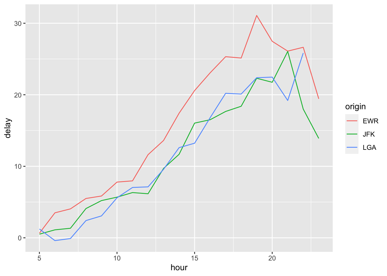

Joins

Databases become more exciting with more tables. So let’s add a couple more:

copy_to(
  dest = con, 
  df = nycflights13::planes, 
  name = "planes",
  temporary = FALSE, 
  indexes = "tailnum"
)

copy_to(
  dest = con, 
  df = nycflights13::airlines, 
  name = "airlines",
  temporary = FALSE, 
  indexes = "carrier"
)

copy_to(
  dest = con, 
  df = nycflights13::airports, 
  name = "airports",
  temporary = FALSE, 
  indexes = "faa"
)

copy_to(
  dest = con, 
  df = nycflights13::weather, 
  name = "weather",
  temporary = FALSE, 
  indexes = list(
    c("year", "month", "day", "hour", "origin")
  )
)

Let us call dbListTables() again on our “con” database connection. As you can see, there are several more tables now.

dbListTables(con)

## [1] "airlines"     "airports"     "flights"      "planes"       "sqlite_stat1"
## [6] "sqlite_stat1" "sqlite_stat4" "sqlite_stat4" "weather"

As we saw last week, the join syntax had its origin in SQL. Unsurprisingly, you can join tables without having to store the data in memory. Here is how you perform a left join:

planes_db = tbl(con, 'planes')
left_join(
  flights_db,
  planes_db %>% rename(year_built = year),
  by = "tailnum" ## Important: Be specific about the joining column
) %>%
  select(year, month, day, dep_time, arr_time, carrier, flight, tailnum,
         year_built, type, model)

This should all feel very familiar right? 😁

A look under the Hood

As you saw, you can conduct your analyses in a database, the same way you are used to do it in R. All that without your data having to be stored on your own device.

Unfortunately, there are however some differences between ordinary data frames and remote database queries that are worth pointing out.

The most important among these is that your R code is translated into SQL and executed in the database on the remote server, not in R on your local machine.

This has the following implications. When working with databases, dplyr tries to be as lazy as possible 😴:

It never pulls data into R unless you explicitly ask for it.
It delays doing any work until the last possible moment: it collects together everything you want to do and then sends it to the database in one step.

This even applies when you assign the output of a database query to an object:

tailnum_delay_db <- flights_db %>% 
  group_by(tailnum) %>%
  summarise(
    delay = mean(arr_delay),
    n = n()
  ) %>% 
  arrange(desc(delay)) %>%
  filter(n > 100)

This leads to some unexpected behaviour:

Exhibit A: Because there’s generally no way to determine how many rows a query will return unless you actually run it, nrow() is always NA.

nrow(tailnum_delay_db)

## [1] NA

Exhibit B: Because you can’t find the last few rows without executing the whole query, you can’t use tail().

tail(tailnum_delay_db)

## Error: tail() is not supported by sql sources

Inspecting queries

We can always inspect the SQL code that dbplyr is generating:

tailnum_delay_db %>% show_query()

## <SQL>
## SELECT *
## FROM (SELECT `tailnum`, AVG(`arr_delay`) AS `delay`, COUNT(*) AS `n`
## FROM `flights`
## GROUP BY `tailnum`)
## WHERE (`n` > 100.0)

That’s probably not how you would write the SQL yourself, but it works.

More information about SQL translation can be found here: vignette("translation-verb").

From remote to local storage

If you then want to pull the data into a local data frame, use collect():

tailnum_delay <- tailnum_delay_db %>% collect()
tailnum_delay

Using SQL directly in R

If, for whatever reason you might want to write your SQL queries yourself, you can use DBI::dbGetQuery() to run SQL queries in R scripts:

sql_query <- "SELECT * FROM flights WHERE dep_delay > 240.0 LIMIT 5"
dbGetQuery(con, sql_query)

If you want to learn more about writing SQL with dbplyr, check out vignette('sql', package = 'dbplyr').

Disconnect from database

When you are done with your SQL queries, it is a good idea to disconnect from the database. What seems evident, becomes increasingly important if you work with servers that charge you for their services!

DBI::dbDisconnect(con)

Exercises on Databases

If you want to practice accessing databases going forward, have a look at the practice script here. It comes with a database file so you can open the connection locally without the need to register. Thanks for the excellent example to our colleague Will Lowe!

(Advanced) BigQuery

If you are still curious about databases and SQL and wonder how you might scale all this up in for the purposes of a real project, you might be interested to look into Google’s BigQuery service. You can register for a free Google Cloud account here. Be aware that you only have a certain amount of free queries (1 TB / month) before you are charged. BigQuery is the most widely used service to interact with online databses and it has a number of public datasets that you can easily practice with. Everything we saw above applies, with the exception that you need to specify the backend bigrquery::bigquery().

Here is an example of how it would look:

con <- dbConnect(
  bigrquery::bigquery(),
  project = "publicdata",
  dataset = "samples",
  billing = google_cloud_project_name # This will tell Google whom to charge
)

Actually learning R 🎒

Let us remind you again, the key to learning R is: Google! We can only give you an overview over basic R functions, but to really learn R you will have to actively use it yourself, trouble shoot, ask questions, and google! It is very likely that someone else has had the exact same or just similar enough issue before and that the R community has answered it with 5+ different solutions years ago. 😉

Sources

The section on functions and iteration is partly based on R for Data Science, section 5.2, Quantitative Politics with R, chapter 3; as well as the Tidyverse Session in the course Data Science for Economists by Grant McDermott. The data for the exercises was inspired by R for Epidemiology

The section on databases and SQL relies on the vignette from the dbplyr package, RStudio Tutorial on databases as well as the Databases Session in McDermott’s Data Science for Economists by Grant McDermott.

A work by Lisa Oswald & Tom Arend

Prepared for Intro to Data Science, taught by Simon Munzert

Hertie School, Berlin

Databases

Functions, dtplyr and working with SQL in R