Today, we’ll finally leave base R behind and make our lives much easier by introducing you to the tidyverse. ✨ We think for data cleaning, wrangling, and plotting, the tidyverse really is a no-brainer. A few good reasons for teaching the tidyverse are:

Outstanding documentation and community support
Consistent philosophy and syntax
Convenient “front-end” for more advanced methods

The Tidyverse 🔭

In general, the tidyverse is a collection of R packages that share an underlying design, syntax, and structure. One very prominent tidyverse package is dplyr for data manipulation.

In this lab, you will learn to:

understand what we mean with tidy data
identify the purpose of a set of dplyr verbs
restructure data with a set of tidyr verbs
learn about functions and iteration with purrr

Tidy Data 🗂

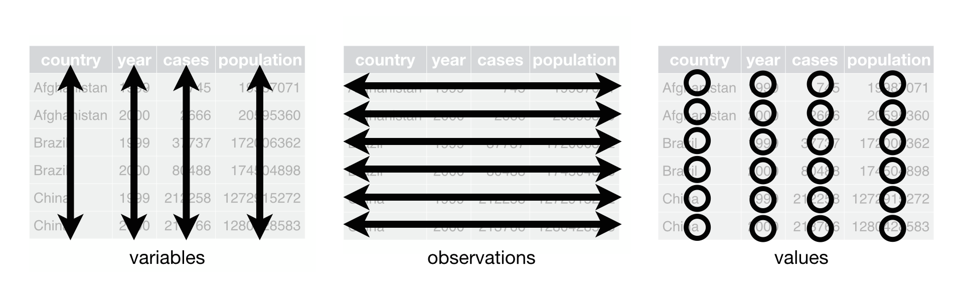
Generally, we will encounter data in a tidy format. Tidy data refers to a way of mapping the structure of a data set. In a tidy data set:

Each variable forms a column.
Each observation forms a row.
Each type of observational unit forms a table

Excercise 1

Think about what you might have learned about panel surveys (surveys fielded to the same set of participants at multiple points of time). Why could this be a problem for the general assumptions of tidy data and what possible data formats can you end up with?

Tidyverse packages

Let’s load the tidyverse meta-package and check the output.

library(tidyverse)

We see that we have actually loaded a number of packages (which could also be loaded individually): ggplot2, tibble, dplyr, etc. We can also see information about the package versions and some namespace conflicts.

The tidyverse actually comes with a lot more packages than those that are just loaded automatically.¹

tidyverse_packages()

##  [1] "broom"         "cli"           "crayon"        "dbplyr"       
##  [5] "dplyr"         "dtplyr"        "forcats"       "googledrive"  
##  [9] "googlesheets4" "ggplot2"       "haven"         "hms"          
## [13] "httr"          "jsonlite"      "lubridate"     "magrittr"     
## [17] "modelr"        "pillar"        "purrr"         "readr"        
## [21] "readxl"        "reprex"        "rlang"         "rstudioapi"   
## [25] "rvest"         "stringr"       "tibble"        "tidyr"        
## [29] "xml2"          "tidyverse"

We’ll use several of these additional packages during the remainder of this course.

E.g. The lubridate package for working with dates and the rvest package for webscraping. However, these packages will have to be loaded separately!

The pipe `%>%` operator

The tidyverse loads its a pipe operator, denoted %>%. Using pipes can dramatically improve the experience of reading and writing code. Compare:

## These next two lines of code do exactly the same thing.

mpg %>% filter(manufacturer=="audi") %>% group_by(model) %>% summarise(hwy_mean = mean(hwy))

summarise(group_by(filter(mpg, manufacturer=="audi"), model), hwy_mean = mean(hwy))

The first line reads from left to right, exactly how I thought of the operations in my head. - Take this object (mpg), do this (filter), then do this (group_by), etc.

The second line totally inverts this logical order (the final operation comes first!) - Who wants to read things inside out?

The piped version of the code is even more readable if we write it over several lines. Here it is again and, this time, I’ll run it for good measure so you can see the output:

mpg %>% 
  filter(manufacturer=="audi") %>% 
  group_by(model) %>% 
  summarise(hwy_mean = mean(hwy))

Remember: Using vertical space costs nothing and makes for much more readable/writeable code than cramming things horizontally.

PS — The pipe is originally from the magrittr package, which can do some other cool things if you’re inclined to explore.

Data manipulation with `dplyr`

In this tutorial, you’ll learn and practice examples using some functions in dplyr to work with data. Those are:

select(): keep or exclude some columns
filter(): keep rows that satisfy your conditions
mutate(): add columns from existing data or edit existing columns
group_by(): lets you define groups within your data set
summarize(): get summary statistics
arrange(): reorders the rows according to single or multiple variables

To demonstrate and practice how these verbs (functions) work, we’ll use the penguings dataset.

The 3 species of penguins in this data set are Adelie, Chinstrap and Gentoo. The data set contains 8 variables:

species: a factor denoting the penguin species (Adelie, Chinstrap, or Gentoo)
island: a factor denoting the island (in Palmer Archipelago, Antarctica) where observed
culmen_length_mm: a number denoting length of the dorsal ridge of penguin bill (millimeters)
culmen_depth_mm: a number denoting the depth of the penguin bill (millimeters)
flipper_length_mm: an integer denoting penguin flipper length (millimeters)
body_mass_g: an integer denoting penguin body mass (grams)
sex: a factor denoting penguin sex (MALE, FEMALE)
year an integer denoting the year of the record

`select()`

The first verb (function) we will utilize is select(). We can employ it to manipulate our data based on columns. If you recall from our initial exploration of the data set there were eight variables attached to every observation. Do you recall them? If you do not, there is no problem. You can utilize names() to retrieve the names of the variables in a data frame.

names(penguins)

## [1] "species"           "island"            "bill_length_mm"   
## [4] "bill_depth_mm"     "flipper_length_mm" "body_mass_g"      
## [7] "sex"               "year"

Say we are only interested in the species, island, and year variables of these data, we can utilize the following syntax:

select(data, columns)

Excercise 2 The following code chunk would select the variables we need. Can you adapt it, so that we keep the body_mass_g and sex variables as well?

dplyr::select(penguins, species, island, year)

Good to know: To drop variables, use - before the variable name, i.e. select(penguins, -year) to drop the year column (select everything but the year column).

`filter()` ☕

The second verb (function) we will employ is filter(). filter() lets you use a logical test to extract specific rows from a data frame. To use filter(), pass it the data frame followed by one or more logical tests. filter() will return every row that passes each logical test.

The more commonly used logical operators are:

==: Equal to
!=: Not equal to
>, >=: Greater than, greater than or equal to
<, <=: Less than, less than or equal to
&, |: And, or

Say we are interested in retrieving the observations from the year 2007. We would do:

dplyr::filter(penguins, year == 2007)

Excercise 3 Can you adapt the code to retrieve all the observations of Chinstrap penguins from 2007

Excercise 4 We can leverage the pipe operator to sequence our code in a logical manner. Can you adapt the following code chunck with the pipe and conditional logical operators we discussed?

only_2009 <- dplyr::filter(penguins, year == 2009)
only_2009_chinstraps <- dplyr::filter(only_2009, species == "Chinstrap")
only_2009_chinstraps_species_sex_year <- dplyr::select(only_2009_chinstraps, species, sex, year)
final_df <- only_2009_chinstraps_species_sex_year
final_df #to print it in our console

`mutate()` 🌂☂️

mutate() lets us create, modify, and delete columns. The most common use for now will be to create new variables based on existing ones. Say we are working with a U.S. American client and they feel more confortable with assessing the weight of the penguins in pounds. We would utilize mutate() as such:

mutate(new_var_name = manipulated old_var(s))

penguins %>%
  dplyr::mutate(body_mass_lbs = body_mass_g/453.6)

`group_by()` and `summarize()`

These two verbs group_by() and summarize() tend to go together. When combined , ’summarize()` will create a new data frame. It will have one (or more) rows for each combination of grouping variables; if there are no grouping variables, the output will have a single row summarising all observations in the input. For example:

# compare this output with the one below
penguins %>%
  dplyr::summarize(heaviest_penguin = max(body_mass_g, na.rm = T))

penguins %>%
  dplyr::group_by(species) %>%
  dplyr::summarize(heaviest_penguin = max(body_mass_g, na.rm = T))

Excercise 5 Can you get the weight of the lightest penguin of each species? You can use min(). What happens when in addition to species you also group by year group_by(species, year)?

penguins %>%
  dplyr::group_by(species, year) %>%
  dplyr::summarize(lightest_penguin = min(body_mass_g, na.rm = T))

`arrange()` 🥚🐣🐥

The arrange() verb is pretty self-explanatory. arrange() orders the rows of a data frame by the values of selected columns in ascending order. You can use the desc() argument inside to arrange in descending order. The following chunk arranges the data frame based on the length of the penguins’ bill. You hint tab contains the code for the descending order alternative.

penguins %>%
  dplyr::arrange(bill_length_mm)

penguins %>%
  dplyr::arrange(desc(bill_length_mm))

Excercise 6 Can you create a data frame arranged by body_mass_g of the penguins observed in the “Dream” island?

Quiz

Which verb allows you to index columns?

select()
filter()
summarize()
group_by()

Which verb allows you to index rows?

select()
filter()
summarize()
group_by()

How long was the longest observed bill of a Gentoo penguin in 2008?
How long was the shortest observed bill of a Gentoo penguin in 2008?

Other dplyr functions

ungroup(): For ungrouping data after using the group_by() command - Particularly useful with the summarise and mutate commands, as we’ve already seen.

slice(): Subset rows by position rather than filtering by values. - E.g. penguins %>% slice(c(1, 5))

pull(): Extract a column from as a data frame as a vector or scalar. - E.g. penguins %>% filter(gender=="female") %>% pull(height)

count() and distinct(): Number and isolate unique observations. - E.g. penguins %>% count(species), or penguins %>% distinct(species) - You could also use a combination of mutate, group_by, and n(), e.g. penguins %>% group_by(species) %>% mutate(num = n()).

The final set of dplyr verbs we’d like you to know are the family of join operations. These are important enough that we want to go over some concepts in a bit more depth.

However - note that we will cover relational data structures (and SQL) in even more depth in a separate lab session!

Joins with `dplyr`

One of the mainstays of the dplyr package is merging data with the family join operations.

inner_join(df1, df2)
left_join(df1, df2)
right_join(df1, df2)
full_join(df1, df2)
semi_join(df1, df2)
anti_join(df1, df2)

(You might find it helpful to to see visual depictions of the different join operations here.)

For the simple examples that I’m going to show here, we’ll need some data sets that come bundled with the nycflights13 package. - Load it now and then inspect these data frames in your own console.

Let’s perform a left join on the flights and planes datasets. - Note: I’m going subset columns after the join, but only to keep text on the slide.

left_join(flights, planes) %>%
  select(year, month, day, dep_time, arr_time, carrier, flight, tailnum, type, model)%>%
  head(3) ## Just to save vertical space in output

Note that dplyr made a reasonable guess about which columns to join on (i.e. columns that share the same name). It also told us its choices:

## Joining, by = c("year", "tailnum")

However, there’s an obvious problem here: the variable “year” does not have a consistent meaning across our joining datasets! - In one it refers to the year of flight, in the other it refers to year of construction.

Luckily, there’s an easy way to avoid this problem. - Try ?dplyr::join.

You just need to be more explicit in your join call by using the by = argument. - You can also rename any ambiguous columns to avoid confusion.

left_join(
  flights,
  planes %>% rename(year_built = year), ## Not necessary w/ below line, but helpful
  by = "tailnum" ## Be specific about the joining column
  ) %>%
  select(year, month, day, dep_time, arr_time, carrier, flight, tailnum, year_built, type, model) %>%
  head(3)

Last thing I’ll mention for now; note what happens if we again specify the join column… but don’t rename the ambiguous “year” column in at least one of the given data frames.

left_join(
  flights,
  planes, ## Not renaming "year" to "year_built" this time
  by = "tailnum"
  ) %>%
  select(contains("year"), month, day, dep_time, arr_time, carrier, flight, tailnum, type, model) %>%
  head(3)

Make sure you know what “year.x” and “year.y” are. Again, it pays to be specific.

Let’s move on to another important tidyverse package!

The `tidyr` package

Key tidyr verbs are:

pivot_longer: Pivot wide data into long format (i.e. “melt”).¹
pivot_wider: Pivot long data into wide format (i.e. “cast”).²
separate: Separate (i.e. split) one column into multiple columns.
unite: Unite (i.e. combine) multiple columns into one.

`pivot_longer()`

stocks = data.frame( ## Could use "tibble" instead of "data.frame" if you prefer
  time = as.Date('2009-01-01') + 0:1,
  X = rnorm(2, 0, 1),
  Y = rnorm(2, 0, 2),
  Z = rnorm(2, 0, 4)
  )
stocks

stocks %>% pivot_longer(-time, names_to="stock", values_to="price")

Let’s quickly save the “tidy” (i.e. long) stocks data frame

## Write out the argument names this time: i.e. "names_to=" and "values_to="
tidy_stocks <- stocks %>% 
  pivot_longer(-time, names_to="stock", values_to="price")

`pivot_wider()`

tidy_stocks %>% pivot_wider(names_from=stock, values_from=price)

tidy_stocks %>% pivot_wider(names_from=time, values_from=price)

Note that the second example; which has combined different pivoting arguments; has effectively transposed the data.

`tidyr::separate()` 💔

economists = data.frame(name = c("Adam.Smith", "Paul.Samuelson", "Milton.Friedman"))
economists

economists %>% separate(name, c("first_name", "last_name"))

This command is pretty smart. But to avoid ambiguity, you can also specify the separation character with separate(..., sep=".").

A related function is separate_rows, for splitting up cells that contain multiple fields or observations (a frustratingly common occurence with survey data).

jobs = data.frame(
  name = c("Jack", "Jill"),
  occupation = c("Homemaker", "Philosopher, Philanthropist, Troublemaker") 
  ) 
jobs

## Now split out Jill's various occupations into different rows
jobs %>% separate_rows(occupation)

`tidyr::unite()` ❤️

gdp = data.frame(
  yr = rep(2016, times = 4),
  mnth = rep(1, times = 4),
  dy = 1:4,
  gdp = rnorm(4, mean = 100, sd = 2)
  )
gdp

## Combine "yr", "mnth", and "dy" into one "date" column
gdp %>% unite(date, c("yr", "mnth", "dy"), sep = "-")

Note that unite will automatically create a character variable. You can see this better if we convert it to a tibble.

gdp_u = gdp %>% unite(date, c("yr", "mnth", "dy"), sep = "-") %>% as_tibble()
gdp_u

If you want to convert it to something else (e.g. date or numeric) then you will need to modify it using mutate. See below for an example, using the lubridate package’s super helpful date conversion functions.

library(lubridate)
gdp_u %>% mutate(date = ymd(date))

Functions

Functions allow you to automate tasks in a more powerful and general way than copy-and-pasting. Writing a function has three big advantages over using copy-and-paste:

You can give a function an evocative name that makes your code easier to understand.
As requirements change, you only need to update code in one place, instead of many.
You eliminate the chance of making incidental mistakes when you copy and paste (i.e. updating a variable name in one place, but not in another).

You can read more on functions in this section of R for Data Science.

Generally, how does code look like that calls for writing a function? For example like this:

df <- data.frame(
  a = rnorm(100, 5, 2),
  b = rnorm(100, 100, 15),
  c = rnorm(100, 2, 1),
  d = rnorm(100, 36, 7)
)

df$a <- (df$a - mean(df$a, na.rm = TRUE)) / sd(df$a, na.rm = TRUE)
df$b <- (df$b - mean(df$b, na.rm = TRUE)) / sd(df$a, na.rm = TRUE) # spot the mistake?
df$c <- (df$c - mean(df$c, na.rm = TRUE)) / sd(df$c, na.rm = TRUE)
df$d <- (df$d - mean(df$d, na.rm = TRUE)) / sd(df$d, na.rm = TRUE)

There are three key steps to creating a new function:

Pick a name for the function. For us it could be zscale because this function rescales (or z-transforms) a vector to have a mean of 0 and a standard deviation of 1.
You list the inputs, or arguments, to the function inside function. Here we have just one argument. If we had more the call would look like function(x, y, z).
You place the code you have developed in body of the function, a { block that immediately follows function(…).

The overall structure of a function looks like this in R:

function_name <- function(input_parameters){
  Do what you want to do in the body of the
  function, just like you would write other code in R.
}

In our example, we could simplify the z-transformation of 4 variables with this function:

zscale <- function(x){
  (x - mean(x, na.rm = T) / sd(x, na.rm = T))
}

A word on function names. Generally, function names should be verbs, and arguments should be nouns. There are some exceptions: nouns are ok if the function computes a very well known noun (i.e. mean), or accessing some property of an object (i.e. coefficients). A good sign that a noun might be a better choice is if you’re using a very broad verb like “get”, “compute”, “calculate”, or “determine”. Where possible, avoid overriding existing functions and variables. However, many good names are already taken by other packages, but avoiding the most common names from base R will avoid confusion.

Conditions

You can of course also add conditions to your function.

if (this) {
  # do that
} else if (that) {
  # do something else
} else {
  # 
}

You could, for example, only transform numeric variables.

zscale <- function(x){
  if (is.numeric(x)) {
  (x - mean(x, na.rm = T) / sd(x, na.rm = T))
  }
}

We can now apply our function to any variable that we would like to transform.

df$a <- zscale(df$a)
df$b <- zscale(df$b)
df$c <- zscale(df$c)
df$d <- zscale(df$d)

# you can also use your function with a pipe!
df$d %>% zscale()

Note that there is still a lot of repetition. We can get rid of this using iteration 👇

Iteration

Iteration helps you when you need to do the same thing to multiple inputs: repeating the same operation on different columns, or on different datasets.

On the one hand, you have for loops and while loops which are a great place to start because they make iteration very explicit. On the other hand, functional programming (FP) offers tools to extract out duplicated code, so each common for loop pattern gets its own function.

Remember the code above - it violates the rule of thumb that you should not copy and paste more than twice.

# repetitive code
df$a <- zscale(df$a)
df$b <- zscale(df$b)
df$c <- zscale(df$c)
df$d <- zscale(df$d)

# equivalent iteration
for (i in seq_along(df)) {       # seq_along() similar to length()
  df[[i]] <- zscale(df[[i]])     # [[]] because we are working on single elements
}

To solve problems like this one with a for loop we again think about the three components:

Output: we already have the output — it’s the same as the input because we are modifying data. If that is not the case, make sure to define a space where the output should go (e.g. an empty vector). If the length of your vector is unknown, you might be tempted to solve this problem by progressively growing the vector. However, this is not very efficient because in each iteration, R has to copy all the data from the previous iterations. In technical terms you get “quadratic” (O(n^2)) behaviour which means that a loop with three times as many elements would take nine (3^2) times as long to run. A better solution to save the results in a list, and then combine into a single vector after the loop is done. See more on this here.
Sequence: we can think about a data frame as a list of columns, so we can iterate over each column with seq_along(df).
Body: apply zscale() or any other function.

Functionals 🐱

For loops are not as important in R as they are in other languages because R is a functional programming language. This means that it’s possible to wrap up for loops in a function, and call that function instead of using the for loop directly. 💡

The purrr package provides functions that eliminate the need for many common for loops. The apply family of functions in base R (apply(), lapply(), tapply(), etc) solve a similar problem, but purrr is more consistent and thus is easier to learn.

The pattern of looping over a vector, doing something to each element and saving the results is so common that the purrr package provides a family of functions to do it for you. There is one function for each type of output:

map() makes a list.
map_lgl() makes a logical vector.
map_int() makes an integer vector.
map_dbl() makes a double vector.
map_chr() makes a character vector.

Each function takes a vector as input, applies a function to each piece, and then returns a new vector that’s the same length (and has the same names) as the input. The type of the vector is determined by the suffix to the map function.

# repetitive code
mean(df$a)
mean(df$b)
mean(df$c)
mean(df$d)

# equivalent map function
map_dbl(df,mean)

# map function in tidyverse style
df %>% map_dbl(mean)

There is, of course, much more to learn about functions in R and we could dedicate an entire session to it. For now, consider this as is the first exposure to functions (that can actually already get you pretty far). However, it is important that you apply 🤓 you new skills and practice further on your own. A good starting point is obviously assignment 2 that is due October 6, 11pm. Good luck! 🤞

Actually learning R 🎒

Let us remind you again, the key to learning R is: Google! We can only give you an overview over basic R functions, but to really learn R you will have to actively use it yourself, trouble shoot, ask questions, and google! It is very likely that someone else has had the exact same or just similar enough issue before and that the R community has answered it with 5+ different solutions years ago. 😉

Sources

This tutorial is partly based on R for Data Science, section 5.2, Quantitative Politics with R, chapter 3; as well as the Tidyverse Session in the course Data Science for Economists by Grant McDermott.

A work by Lisa Oswald & Tom Arend

Prepared for Intro to Data Science, taught by Simon Munzert

Hertie School, Berlin

Tidyverse

Data cleaning, wrangling and plotting in R

The Tidyverse 🔭

Tidy Data 🗂

Tidyverse packages

The pipe %>% operator

Data manipulation with dplyr

select()

filter() ☕

mutate() 🌂☂️

group_by() and summarize()

arrange() 🥚🐣🐥