Problem Set 2

01 Loading packages…

# Packages
pacman::p_load(fastverse, fixest, here)
fastverse_extend(topics = 'VI')

-- [1mAttaching extension packages[22m ----------------------------- [38;5;33mfastverse[39m 0.2.1 --

[38;5;33mv[39m [38;5;198mggplot2[39m 3.3.5       [38;5;33mv[39m [38;5;198mlattice[39m 0.20.44
[38;5;33mv[39m [38;5;198mscales [39m 1.1.1       [38;5;33mv[39m [38;5;198mgrid   [39m 4.1.1

-- [1mConflicts[22m ------------------------------------------ fastverse_conflicts() --
[31mx[39m [34mscales[39m::[32mpvalue()[39m masks [34mfixest[39m::pvalue()

# Load data
ps_dt = here('data-002.csv') %>% fread()

02 Time for some figures.

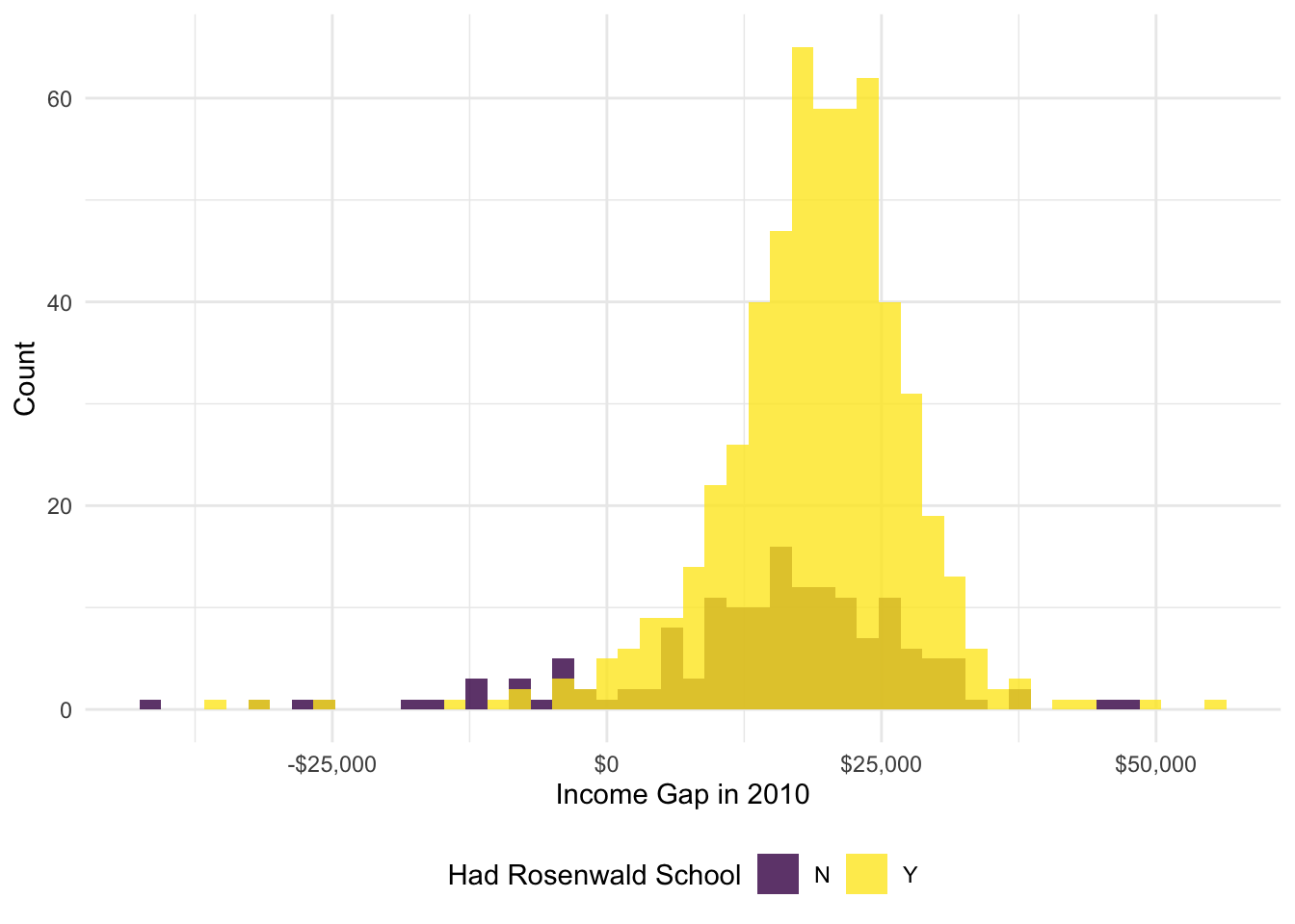
# Black income, 2010
ggplot(
  data = ps_dt,
  aes(x = income_white_2010 - income_black_2010, fill = as.factor(had_rosenwald_school))
) +
geom_histogram(alpha = 0.8, color = NA, position = 'identity', bins = 50) +
scale_fill_viridis_d('Had Rosenwald School', labels = c('N', 'Y')) +
scale_x_continuous('Income Gap in 2010', labels = dollar) +
scale_y_continuous('Count', labels = comma) +
theme_minimal() +
theme(legend.position = 'bottom')

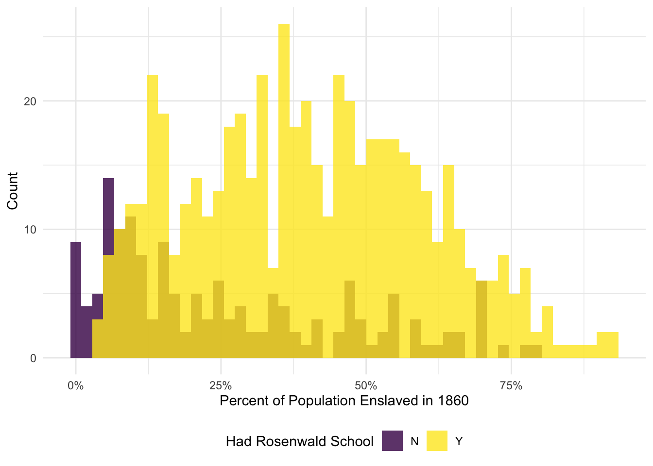
# Black income, 2010
ggplot(
  data = ps_dt,
  aes(x = pct_pop_enslaved_1860/100, fill = as.factor(had_rosenwald_school))
) +
geom_histogram(alpha = 0.8, color = NA, position = 'identity', bins = 50) +
scale_fill_viridis_d('Had Rosenwald School', labels = c('N', 'Y')) +
scale_x_continuous('Percent of Population Enslaved in 1860', labels = percent) +
scale_y_continuous('Count', labels = comma) +
theme_minimal() +
theme(legend.position = 'bottom')

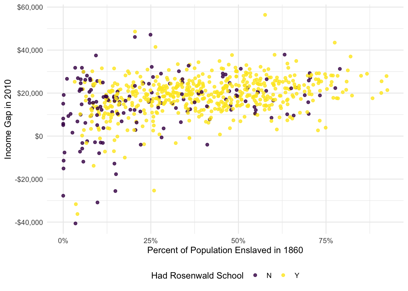
# Black income, 2010
ggplot(
  data = ps_dt,
  aes(x = pct_pop_enslaved_1860/100, y = income_white_2010 - income_black_2010, color = as.factor(had_rosenwald_school))
) +
geom_point(alpha = 0.8) +
scale_color_viridis_d('Had Rosenwald School', labels = c('N', 'Y')) +
scale_x_continuous('Percent of Population Enslaved in 1860', labels = percent) +
scale_y_continuous('Income Gap in 2010', labels = dollar) +
theme_minimal() +
theme(legend.position = 'bottom')

03 Regressing the income gap on the indicator for Rosenwald school, we are assuming that schools’ locations are as good as random (in their distribution across counties). In other words, we need anything that affects the gap—other than the schools—to be independent of whether counties had Rosenwald schools.

# Cross-sectional regression
reg03 = feols(
  income_white_2010 - income_black_2010 ~ 
  had_rosenwald_school,
  data = ps_dt
)
etable(reg03)

                                                   reg03
Dependent Var.:      income_white_2010-income_black_2010
                                                        
(Intercept)                          14,537.5*** (802.8)
had_rosenwald_school                  4,323.7*** (909.7)
____________________      ______________________________
S.E. type                                            IID
Observations                                         710
R2                                               0.03092
Adj. R2                                          0.02955
---
Signif. codes: 0 '***' 0.001 '**' 0.01 '*' 0.05 '.' 0.1 ' ' 1

04 Estimates below. Our CIA updates to within state placement of schools needs to be as good as random (conditional on state, all non-Rosenwald school determinants of the income gap are independent of whether or not a county had a Rosenwald school).

# Add state fixed effects
reg04 = feols(
  income_white_2010 - income_black_2010 ~ 
  had_rosenwald_school | 
  state,
  data = ps_dt
)
etable(reg04)

                                                   reg04
Dependent Var.:      income_white_2010-income_black_2010
                                                        
had_rosenwald_school                 4,285.8** (1,087.0)
Fixed-Effects:            ------------------------------
state                                                Yes
____________________      ______________________________
S.E.: Clustered                                by: state
Observations                                         710
R2                                               0.09778
Within R2                                        0.02938
---
Signif. codes: 0 '***' 0.001 '**' 0.01 '*' 0.05 '.' 0.1 ' ' 1

05 Estimates below…

# Add 1860 controls
reg05 = feols(
  income_white_2010 - income_black_2010 ~ 
  had_rosenwald_school + pct_pop_enslaved_1860 + pop_total_1860 | 
  state,
  data = ps_dt
)
etable(reg05)

                                                    reg05
Dependent Var.:       income_white_2010-income_black_2010
                                                         
had_rosenwald_school                    2,252.9** (669.1)
pct_pop_enslaved_1860                    129.1*** (20.06)
pop_total_1860                           0.1062* (0.0409)
Fixed-Effects:             ------------------------------
state                                                 Yes
_____________________      ______________________________
S.E.: Clustered                                 by: state
Observations                                          710
R2                                                0.16186
Within R2                                         0.09831
---
Signif. codes: 0 '***' 0.001 '**' 0.01 '*' 0.05 '.' 0.1 ' ' 1

06 Comparison below. Yes, the movement in the point estimate for the effect of Rosenwald schools seems to match what we would expect. One would like expect that places with more histories of more intense slavery would have larger income gaps today and would also have been more likely to receive a Rosenwald school. When we control for the county’s history of slavery (and total population in 1860), we see the coefficient on the Rosenwald school indicator decrease.

etable(reg04, reg05)

                                                    reg04
Dependent Var.:       income_white_2010-income_black_2010
                                                         
had_rosenwald_school                  4,285.8** (1,087.0)
pct_pop_enslaved_1860                                    
pop_total_1860                                           
Fixed-Effects:             ------------------------------
state                                                 Yes
_____________________      ______________________________
S.E.: Clustered                                 by: state
Observations                                          710
R2                                                0.09778
Within R2                                         0.02938

                                                    reg05
Dependent Var.:       income_white_2010-income_black_2010
                                                         
had_rosenwald_school                    2,252.9** (669.1)
pct_pop_enslaved_1860                    129.1*** (20.06)
pop_total_1860                           0.1062* (0.0409)
Fixed-Effects:             ------------------------------
state                                                 Yes
_____________________      ______________________________
S.E.: Clustered                                 by: state
Observations                                          710
R2                                                0.16186
Within R2                                         0.09831
---
Signif. codes: 0 '***' 0.001 '**' 0.01 '*' 0.05 '.' 0.1 ' ' 1

07 Open answer: Just want to see a DAG that makes the point that we have likely not controlled for everything.

08 I’d be concerned that there could be a bad-controls issue here: if the schools affected current (or 2010) population levels, then we should not control for it. If we don’t think schools affected current population, then we are probably fine (depending on the DAG you have in mind).

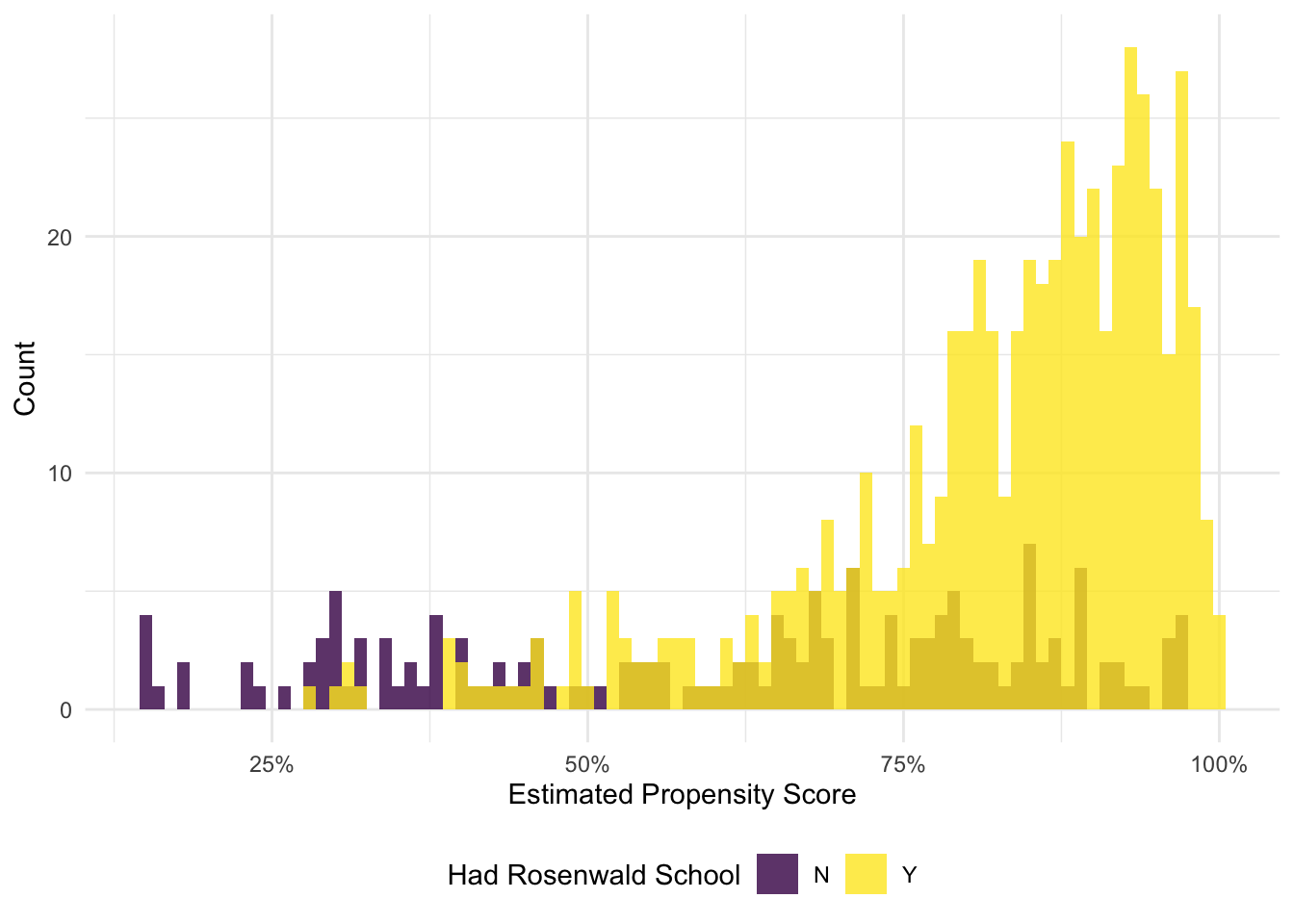
09 Estimate the propensity scores…

# Estimate propensity scores as function of 1860 attributes
pscore_reg = feglm(
  had_rosenwald_school ~ 
  #pct_pop_enslaved_1860 + pop_total_1860,
  I(pct_pop_enslaved_1860^2) + I(pop_total_1860^2) + pct_pop_enslaved_1860 * pop_total_1860,
  data = ps_dt,
  family = 'logit'
)
# Add propensity scores to the dataset
ps_dt[, p_score := predict(pscore_reg, newdata = ps_dt)]

10 Estimates below. The estimated effect of Rosenwald schools is smaller in magnitude and no longer significantly different from zero (still positive).

# Estimate the 1860-controls regression, controlling for the propensity score
reg10 = feols(
  income_white_2010 - income_black_2010 ~ 
  had_rosenwald_school + pct_pop_enslaved_1860 + pop_total_1860 + p_score | 
  state,
  data = ps_dt
)
etable("OLS" = reg05, "Prop. Scores" = reg10)

                                                      OLS
Dependent Var.:       income_white_2010-income_black_2010
                                                         
had_rosenwald_school                    2,252.9** (669.1)
pct_pop_enslaved_1860                    129.1*** (20.06)
pop_total_1860                           0.1062* (0.0409)
p_score                                                  
Fixed-Effects:             ------------------------------
state                                                 Yes
_____________________      ______________________________
S.E.: Clustered                                 by: state
Observations                                          710
R2                                                0.16186
Within R2                                         0.09831

                                             Prop. Scores
Dependent Var.:       income_white_2010-income_black_2010
                                                         
had_rosenwald_school                      1,626.8 (928.2)
pct_pop_enslaved_1860                     95.69** (23.67)
pop_total_1860                           0.0619. (0.0317)
p_score                                 7,464.5 (4,561.5)
Fixed-Effects:             ------------------------------
state                                                 Yes
_____________________      ______________________________
S.E.: Clustered                                 by: state
Observations                                          710
R2                                                0.16806
Within R2                                         0.10498
---
Signif. codes: 0 '***' 0.001 '**' 0.01 '*' 0.05 '.' 0.1 ' ' 1

11 Checking overlap… doesn’t look perfect (yet).

# Check overlap
ggplot(
  data = ps_dt,
  aes(x = p_score, fill = as.factor(had_rosenwald_school))
) +
geom_histogram(alpha = 0.8, color = NA, position = 'identity', binwidth = 0.01) +
scale_fill_viridis_d('Had Rosenwald School', labels = c('N', 'Y')) +
scale_x_continuous('Estimated Propensity Score', labels = percent) +
scale_y_continuous('Count', labels = comma) +
theme_minimal() +
theme(legend.position = 'bottom')

12 Finding the violators.

# Enforce overlap
c_max = ps_dt[had_rosenwald_school == 0, max(p_score)]
t_min = ps_dt[had_rosenwald_school == 1, min(p_score)]
ps_dt[, overlap := 1]
ps_dt[had_rosenwald_school == 0 & p_score < t_min, overlap := 0]
ps_dt[had_rosenwald_school == 1 & p_score > c_max, overlap := 0]

Approximately 93.9% of the observations comply with our enforced overlap.

13 We need to be able to compare individuals with equal likelihoods of treatment. Without overlap, there is no counterfactual for some observations—and we cannot enforce the CIA.

14 Enforcing overlap here doesn’t actually change much…

# Repeat regression but now enforcing overlap
reg14 = feols(
  income_white_2010 - income_black_2010 ~ 
  had_rosenwald_school + pct_pop_enslaved_1860 + pop_total_1860 + p_score | 
  state,
  data = ps_dt[overlap == TRUE]
)
etable('No overlap' = reg10, 'Overlap' = reg14)

                                               No overlap
Dependent Var.:       income_white_2010-income_black_2010
                                                         
had_rosenwald_school                      1,626.8 (928.2)
pct_pop_enslaved_1860                     95.69** (23.67)
pop_total_1860                           0.0619. (0.0317)
p_score                                 7,464.5 (4,561.5)
Fixed-Effects:             ------------------------------
state                                                 Yes
_____________________      ______________________________
S.E.: Clustered                                 by: state
Observations                                          710
R2                                                0.16806
Within R2                                         0.10498

                                                  Overlap
Dependent Var.:       income_white_2010-income_black_2010
                                                         
had_rosenwald_school                      1,622.6 (920.9)
pct_pop_enslaved_1860                     95.13** (23.88)
pop_total_1860                            0.0024 (0.1019)
p_score                                 8,365.2 (5,651.1)
Fixed-Effects:             ------------------------------
state                                                 Yes
_____________________      ______________________________
S.E.: Clustered                                 by: state
Observations                                          667
R2                                                0.16321
Within R2                                         0.09459
---
Signif. codes: 0 '***' 0.001 '**' 0.01 '*' 0.05 '.' 0.1 ' ' 1

15 The coefficient increases a bit when we inversely weight with the estimated propensity scores; it is marginally significant (at the 10% level).

# Add propensity score weights to the dataset
ps_dt[, p_weight := (
  had_rosenwald_school / p_score + (1 - had_rosenwald_school) / (1 - p_score)
)]
# Weighted regression (with controls; no propensity score)
reg15 = feols(
  income_white_2010 - income_black_2010 ~ 
  had_rosenwald_school + pct_pop_enslaved_1860 + pop_total_1860 | 
  state,
  weights = ~ p_weight,
  data = ps_dt[overlap == TRUE]
)
etable(reg15)

                                                    reg15
Dependent Var.:       income_white_2010-income_black_2010
                                                         
had_rosenwald_school                     1,966.4. (941.6)
pct_pop_enslaved_1860                     147.5** (34.88)
pop_total_1860                            0.1026 (0.1497)
Fixed-Effects:             ------------------------------
state                                                 Yes
_____________________      ______________________________
S.E.: Clustered                                 by: state
Observations                                          667
R2                                                0.17514
Within R2                                         0.09152
---
Signif. codes: 0 '***' 0.001 '**' 0.01 '*' 0.05 '.' 0.1 ' ' 1

# Estimate block-level treatement effects
block_dt = lapply(
  X = seq(0.4, 1, 0.1),
  FUN = function(b) {
    # The block's results
    b_est = feols(
      income_white_2010 - income_black_2010 ~ 
      had_rosenwald_school + pct_pop_enslaved_1860 + pop_total_1860 | state,
      data = ps_dt[overlap == TRUE & p_score > b - 0.1 & p_score <= b]
    )
    # Return 
    data.table(
      block = b,
      est =  as.matrix(b_est$coeftable)["had_rosenwald_school","Estimate"],
      n = b_est$nobs
    )
  }
) %>% rbindlist()
# Show block-level treatment effects
block_dt

   block         est   n
1:   0.4 -6248.40100  25
2:   0.5  4740.73301  29
3:   0.6   -40.67093  36
4:   0.7 -5330.11593  66
5:   0.8  4501.95411 114
6:   0.9   179.68589 206
7:   1.0  2780.19632 182

# Estimate the average treatment effect
block_dt[, weighted.mean(x = est, w = n)]

[1] 1039.899

17 The proposed instrument is likely invalid: While it is probably relevant (Rosenwald schools correlates with the county’s level of 1860 enslavement), it is likely not exogenous. There are likely other factors caused by (or related to) slavery that affect the income gap (other than Rosenwald school construction), which violates the exclusion restriction. Further, there may even be a concern about monotonicity if history of enslavement increased some counties’ likelihood of getting a school and decreased other counties.