# Packages
library(pacman)
p_load(
  tidyverse, hrbrthemes, patchwork, data.table, tidymodels,
  embed, ClusterR, parallel, magrittr, here
)
# Load the training dataset
train_dt = here('train.csv') %>% fread()
# Load the testing dataset
test_dt = here('test.csv') %>% fread()Predicting digits
Setup
Let’s get started by loading packages and data for the Digit Recognizer Kaggle competition.
As before, we want to integrate Kaggle’s split into the tidymodels framework (specifically rsample).
- Join the data together.
- Use
make_splits()to create a split object.
# Join the datasets together
all_dt = rbindlist(
  list(train_dt, test_dt),
  use.names = TRUE, fill = TRUE
)
# Find indices of training and testing datasets
i_train = 1:nrow(train_dt)
i_test = (nrow(train_dt)+1):nrow(all_dt)
# Define the custom-split object
kaggle_split = make_splits(
  x = list(analysis = i_train, assessment = i_test),
  data = all_dt
)
# Impose the split (yes, this is redundant)
train_dt = kaggle_split %>% training()
Examples
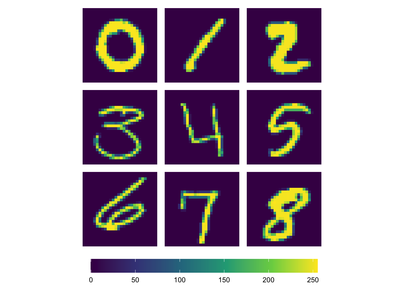
What do the data look like? Let’s plot a few examples.
# Create an example plot for each integer
gg = lapply(X = c(2,1,17,8,4,9,22,7,11,12), FUN = function(i) {
  ggplot(
    data = expand_grid(
      y = 28:1,
      x = 1:28
    ) %>% mutate(value = train_dt[i,-"label"] %>% unlist()),
    aes(x = x, y = y, fill = value)
  ) +
  geom_raster() +
  scale_fill_viridis_c("") +
  theme_void() +
  theme(legend.position = "bottom") +
  coord_equal()
})
# Create a grid of examples
(gg[[1]] + gg[[2]] + gg[[3]]) /
  (gg[[4]] + gg[[5]] + gg[[6]]) /
  (gg[[7]] + gg[[8]] + gg[[9]]) +
  plot_layout(guides = "collect") &
  theme(
    legend.position = "bottom",
    legend.key.width = unit(2, "cm")
  )
Cleaning and recipes
The data are already quite clean (check for yourself), so our only real recipe step is to convert the outcome to factor. (Why?)
# Set up a recipe to create a factor of the label
simple_recipe =
  recipe(label ~ ., data = train_dt) %>%
  step_mutate(label = as.factor(label))
K-means clustering
Pretty much everything we’ve done in this class so far has used supervised learning algorithms—algorithms that train using known labels/outcomes.
Today we’re going to try a classic unsupervised algorithm called K-means clustering.
K-means clustering is a simple algorithm that divides your observations into K distinct groups (A.K.A. clusters).
Rule: Each observation belongs to one—and only one—cluster.
Goal: “Good” clusters have very similar observations. “Bad clusters” have very different observations.
So now we just need to figure out how to measure observations’ similarity—and then move like observations into the same cluster.
Let \(W(C_k)\) denote some arbitrary measure of “within cluster variation” for cluster \(C_k\). A good cluster will have low \(C_k\).
Now remember that we want all clusters to have low within-cluster variation—not just one cluster.
So our goal is \[ \underset{{C_{1},\, \ldots,\, C_{k}}}{\text{minimize}} \sum_{k=1}^{K} W(C_k) \]
As we discussed in the SVM lecture, there are many ways to measure observations’ similarity. A common (easy) way to measure similarity is squared Euclidean distance, i.e., how far apart two observations are in predictor space:
Two dimensions: \[(x_{i,1} - x_{i',1})^2 + (x_{i,2} - x_{i',2})^2\]
\(p\) dimensions: \[\sum_{j=1}^p (x_{i,j} - x_{i',j})^2\]
We then “just” find the squared Euclidean distance between each pair of observations in cluster \(k\) (and divide by \(|C_k|\), the number of observations in cluster \(C_k\) to control for its size).
\[\dfrac{1}{|C_{k}|}\sum_{i,i' \in C_{k}}\sum_{j=1}^p (x_{i,j} - x_{i',j})^2\]
Finally, we repeat this within-cluster variation calculation for every cluster… and try to find the clustering that minimizes the total within-cluster variation.
The algorithm for finding the “best” clustering tends to look like:
- Randomly assign a cluster (\(\{1,\,\ldots,\, K\}\)) to each observation. (Randomly initialize clusters.)
- Calculate the centroid of each cluster.
- Re-assign observations to the cluster with the nearest centroid.
- Repeat steps 2/3 until no more changes occur.
- Possibly repeat the whole process a few times to make sure the clustering is fairly stable (we’re hoping for a global optimum, but the algorithm only ensures local).
Let’s use the KMeans_arma() function from the ClusterR package to calculate 10 clusters (since we know that we have 10 digits). This function only outputs the centroids, but we can then use the centroids to make predictions onto our dataset (assigning the observations to clusters). Think of the clusters’ centroids as our trained \(\hat{f}\), and now we’re getting predictions.
Note: I’m not using the standard kmeans() function because it is much slower (and our current dataset is fairly large).
# Find the 'optimal' centroids
kmeans_train = KMeans_arma(
  data = train_dt %>% select(-label),
  clusters = 10
)
# Add cluster to the training dataset
train_dt[, `:=`(
  cl_k = predict_KMeans(
    data = train_dt %>% select(-label),
    CENTROIDS = kmeans_train
  )
)]
Important: Because K-means is an unsupervised algorithm, the cluster’s number is meaningless. However, in our case, we actually want to know whether the clusters tend to make sense (we’re using an unsupervised algorithm for a supervised prediction problem). So let’s find the most-common (modal) label for each cluster. I’m going to use the fmode() function from the collapse package.
# Find clusters' modal label
train_dt[, `:=`(
  pred = collapse::fmode(label)
), cl_k]
Let’s see how well we did! (Note: We’re still looking at the training sample, but we’re a bit less prone to overfitting, since our algorithm did not train on the label.)
train_dt[,mean(label == pred)][1] 0.5948095Meh. Not amazing (my random forest had 92% OOB accuracy). But not terrible (the null classifier would get 11% correct).
Thinking about the confusion matrix, we can dig into these predictions and their general accuracy a bit more.
Here’s a take on precision: When we guess a number, how often are we correct?
train_dt[, .(accuracy=mean(label == pred), .N), pred] %>% arrange(pred) pred accuracy N
<int> <num> <int>
1: 0 0.7982228 4614
2: 1 0.6331222 7264
3: 2 0.9096292 3209
4: 3 0.5289348 5426
5: 6 0.7228157 5242
6: 7 0.4313121 5838
7: 8 0.5926714 4230
8: 9 0.3394852 6177Notice anything strange?
[1] Some of our guesses are quite bad (when we guess 9—we’re doing that way too often).
[2] We never actually guessed 5 (or 4). Why? Because there is no cluster whose modal outcome is a 5 (or 4):
train_dt[, .(mode=collapse::fmode(label)), .(cluster=cl_k)] %>% arrange(mode) cluster mode
<num> <int>
1: 9 0
2: 4 0
3: 3 1
4: 10 2
5: 8 3
6: 7 6
7: 5 6
8: 2 7
9: 6 8
10: 1 9Let’s compare the “average” of all pixels for things we think are 9s (low precision) to things that are actually 9s.
# Average of things we think are 9s
guess9 = ggplot(
  data = expand_grid(
    y = 28:1,
    x = 1:28
  ) %>% mutate(
    value = train_dt[pred == 9] %>% select(starts_with('pixel')) %>% as.matrix() %>% apply(2, mean)
  ),
  aes(x = x, y = y, fill = value)
) +
geom_raster() +
scale_fill_viridis_c("", limits = c(0,256)) +
theme_void() +
theme(
  legend.position = "bottom"
) +
coord_equal() +
ggtitle("Guessed 9")

is9 = ggplot(
  data = expand_grid(
    y = 28:1,
    x = 1:28
  ) %>% mutate(
    value = train_dt[label == 9] %>% select(starts_with('pixel')) %>% as.matrix() %>% apply(2, mean)
  ),
  aes(x = x, y = y, fill = value)
) +
geom_raster() +
scale_fill_viridis_c("", limits = c(0,256)) +
theme_void() +
theme(
  legend.position = "bottom"
) +
coord_equal() +
ggtitle("Is 9")

misguess9 = ggplot(
  data = expand_grid(
    y = 28:1,
    x = 1:28
  ) %>% mutate(
    value = train_dt[pred == 9 & label != 9] %>% select(starts_with('pixel')) %>% as.matrix() %>% apply(2, mean)
  ),
  aes(x = x, y = y, fill = value)
) +
geom_raster() +
scale_fill_viridis_c("", limits = c(0,256)) +
theme_void() +
theme(
  legend.position = "bottom"
) +
coord_equal() +
ggtitle("Mis-guessed 9")

guess9 + is9 + misguess9 +
plot_layout(guides = "collect") &
theme(
  legend.position = "bottom",
  legend.key.width = unit(2, "cm")
)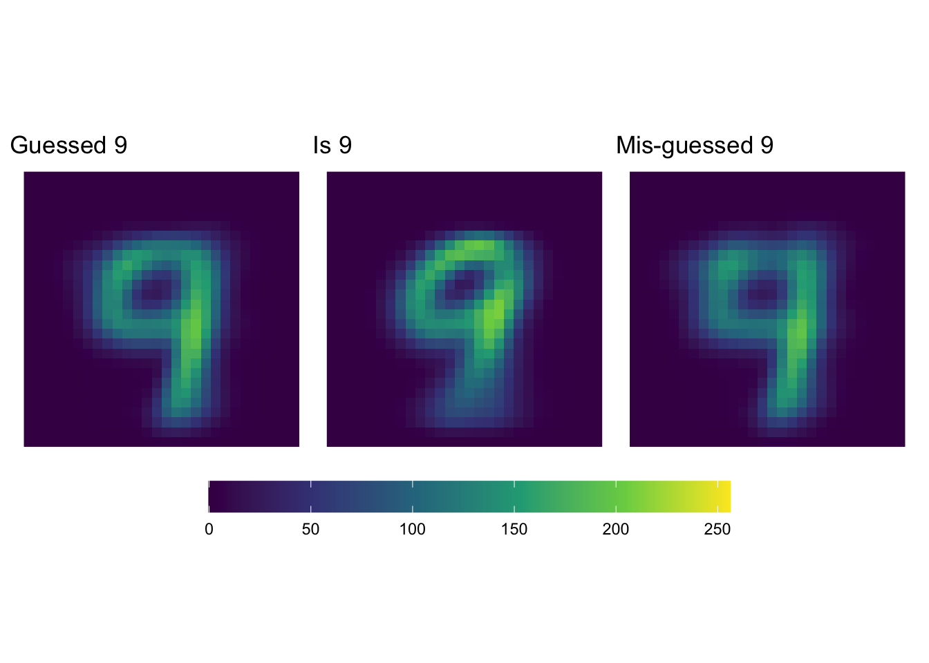
It really doesn’t seem like we’re doing terribly.
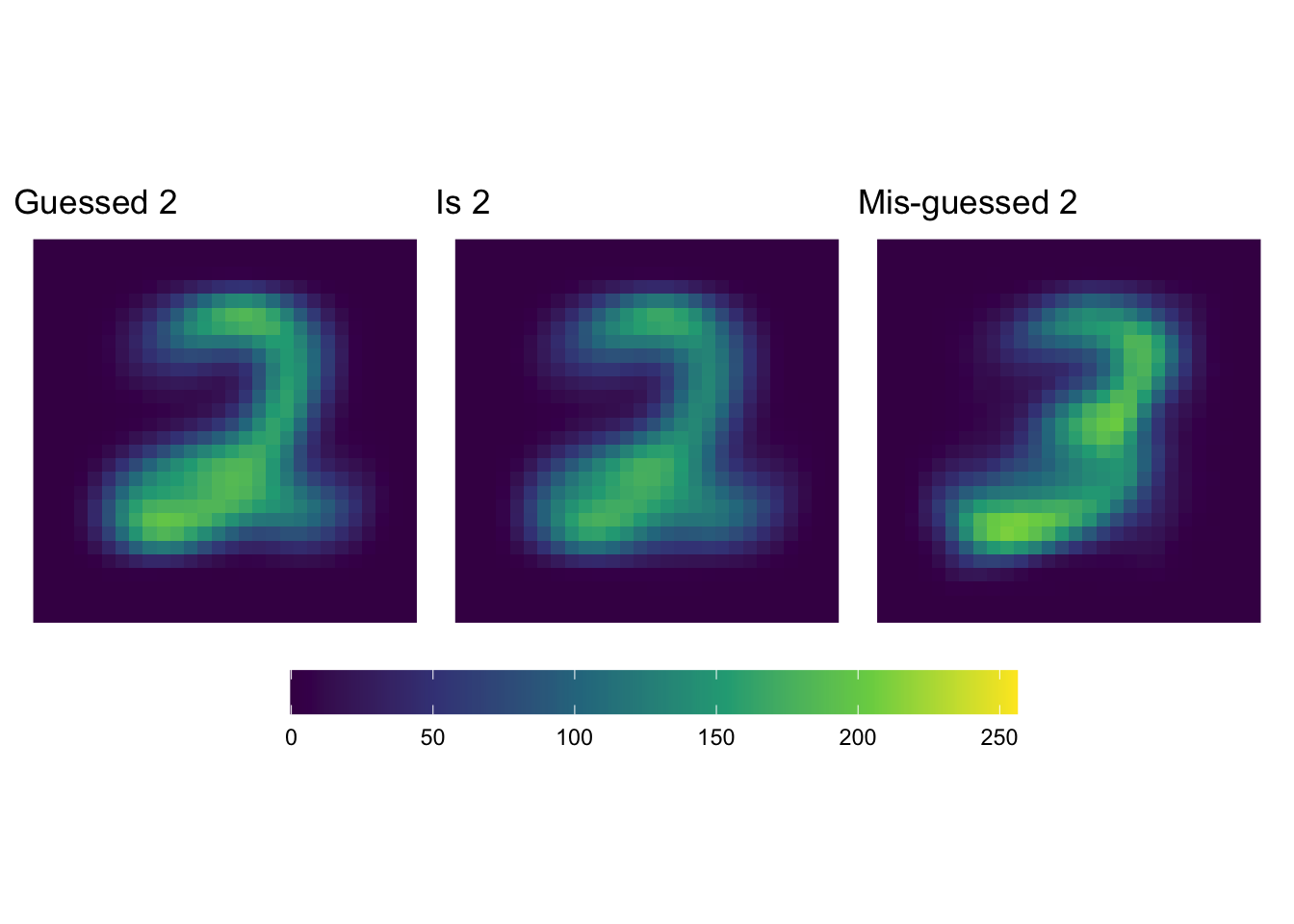
Now let’s see what our higher precision “2” guesses look like…
# Average of things we think are 2s
guess2 = ggplot(
  data = expand_grid(
    y = 28:1,
    x = 1:28
  ) %>% mutate(
    value = train_dt[pred == 2] %>% select(starts_with('pixel')) %>% as.matrix() %>% apply(2, mean)
  ),
  aes(x = x, y = y, fill = value)
) +
geom_raster() +
scale_fill_viridis_c("", limits = c(0,256)) +
theme_void() +
theme(
  legend.position = "bottom"
) +
coord_equal() +
ggtitle("Guessed 2")

misguess2 = ggplot(
  data = expand_grid(
    y = 28:1,
    x = 1:28
  ) %>% mutate(
    value = train_dt[pred == 2 & label != 2] %>% select(starts_with('pixel')) %>% as.matrix() %>% apply(2, mean)
  ),
  aes(x = x, y = y, fill = value)
) +
geom_raster() +
scale_fill_viridis_c("", limits = c(0,256)) +
theme_void() +
theme(
  legend.position = "bottom"
) +
coord_equal() +
ggtitle("Mis-guessed 2")

is2 = ggplot(
  data = expand_grid(
    y = 28:1,
    x = 1:28
  ) %>% mutate(
    value = train_dt[label == 2] %>% select(starts_with('pixel')) %>% as.matrix() %>% apply(2, mean)
  ),
  aes(x = x, y = y, fill = value)
) +
geom_raster() +
scale_fill_viridis_c("", limits = c(0,256)) +
theme_void() +
theme(
  legend.position = "bottom"
) +
coord_equal() +
ggtitle("Is 2")

guess2 + is2 + misguess2 +
plot_layout(guides = "collect") &
theme(
  legend.position = "bottom",
  legend.key.width = unit(2, "cm")
)
What’s K?
Ten clusters seems to make sense in this setting: there are 10 different numbers. Here’s how accurate we are (in sample) when we guess each number:
We assumed that we knew \(K\) (the number of clusters), but maybe we were wrong (maybe handwritten digits don’t divide nicely into exactly 10 groups). And even if we weren’t wrong, it would be nice to know that. Plus… most unsupervised settings don’t give you a priori knowledge of \(K\).
So what should we do?
Try a bunch of values for \(K\)! For now, \(K\) is our only hyperparameter, and we know what to do with hyperparameters… tune those puppies!
The classic approach here is to look at the “total within-cluster variation” as you increase the number of clusters. The total within-cluster variation will always decrease when you add another cluster, so we’re going to try to find the spot where there appear to be decreasing returns to adding more clusters. This approach is sometimes called the “elbow approach”—you’re looking for K at the elbox, where the more clusters stop yielding steep decreases in within-cluster variance.
In our situation, we are actually interested in model accuracy. So let’s check out the accuracy of clusters’ predictions (in-sample, for now) as we increase the number of clusters.
find_k = mclapply(
  mc.cores = parallel::detectCores(),
  X = 1:40,
  FUN = function(k) {
    # Try 'k' clusters
    k_centers = KMeans_arma(
      data = train_dt %>% select(starts_with('pixel')),
      clusters = k
    )
    # Add cluster to the training dataset
    k_dt = data.table(
      label = train_dt[,label],
      cl = predict_KMeans(
        data = train_dt %>% select(starts_with('pixel')),
        CENTROIDS = k_centers
      )
    )
    # Find modal label for each cluster
    k_dt[, pred := collapse::fmode(label), cl]
    # Return a data table with accuracy
    data.table(
      k = k,
      accuracy = k_dt[,mean(label == pred)]
    )
  }
) %>% rbindlist()
And now we can plot our performance as a function of K.
ggplot(
  data = find_k,
  aes(x = k, y = accuracy)
) +
geom_hline(yintercept = 0, size = 1/5) +
geom_line(size = 1/4) +
geom_point(size = 2.5) +
theme_minimal() +
scale_y_continuous('Accuracy', labels = scales::percent, limits = c(0, 1))
Warning: Using `size` aesthetic for lines was deprecated in ggplot2 3.4.0.
ℹ Please use `linewidth` instead.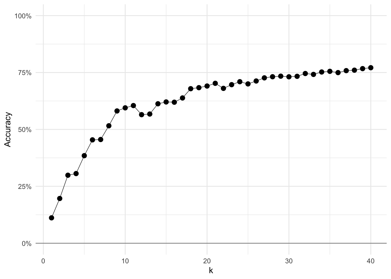
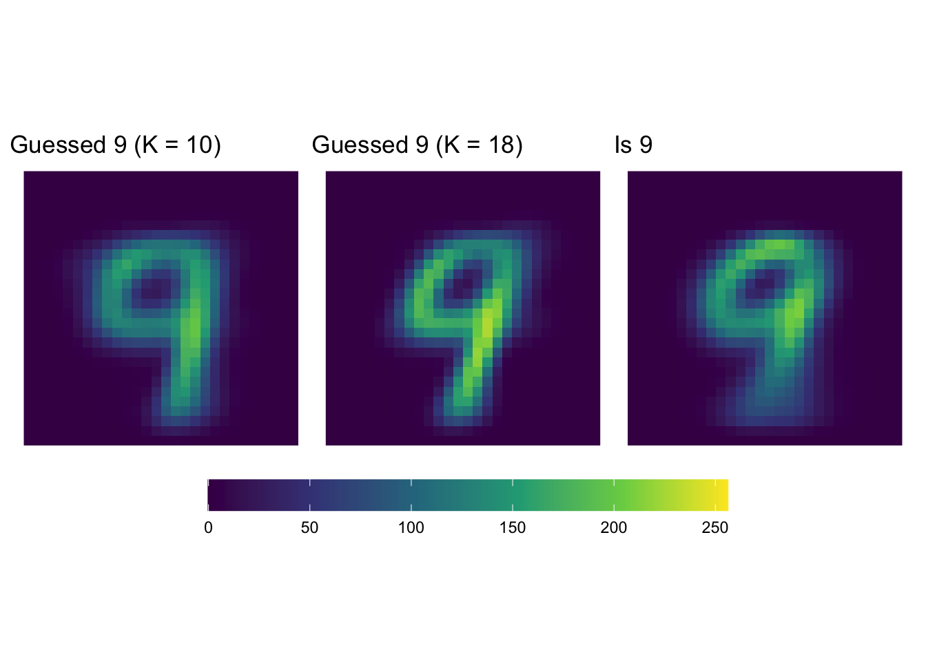
Let’s see how our precision is looking… I’m going to go with 18 clusters.
# Find the 'optimal' centroids
kmeans_train = KMeans_arma(
  data = train_dt %>% select(-label),
  clusters = 18
)
# Add cluster to the training dataset
train_dt[, `:=`(
  cl18 = predict_KMeans(
    data = train_dt %>% select(-label),
    CENTROIDS = kmeans_train
  )
)]
# Find clusters' modal label
train_dt[, `:=`(
  pred18 = collapse::fmode(label)
), cl18]
train_dt[, .(accuracy=mean(label == pred18), .N), pred18] %>% arrange(pred18) pred18 accuracy N
<int> <num> <int>
1: 0 0.9352538 3645
2: 1 0.8375551 5448
3: 2 0.9138335 3412
4: 3 0.5736000 5000
5: 4 0.4685733 3007
6: 5 0.3698516 4783
7: 6 0.8739726 4015
8: 7 0.7161168 4759
9: 8 0.6353542 4503
10: 9 0.4687865 3428# Average of things we think are 9s
guess9_18 = ggplot(
data = expand_grid(
y = 28:1,
x = 1:28
) %>% mutate(
value = train_dt[pred18 == 9] %>% select(starts_with('pixel')) %>% as.matrix() %>% apply(2, mean)
),
aes(x = x, y = y, fill = value)
) +
geom_raster() +
scale_fill_viridis_c("", limits = c(0,256)) +
theme_void() +
theme(
legend.position = "bottom"
) +
coord_equal() +
ggtitle("Guessed 9 (K = 18)")
(guess9 + ggtitle('Guessed 9 (K = 10)')) + guess9_18 + is9 +
plot_layout(guides = "collect") &
theme(
legend.position = "bottom",
legend.key.width = unit(2, "cm")
)
# Average of things we think are 9s
guess2_18 = ggplot(
data = expand_grid(
y = 28:1,
x = 1:28
) %>% mutate(
value = train_dt[pred18 == 2] %>% select(starts_with('pixel')) %>% as.matrix() %>% apply(2, mean)
),
aes(x = x, y = y, fill = value)
) +
geom_raster() +
scale_fill_viridis_c("", limits = c(0,256)) +
theme_void() +
theme(
legend.position = "bottom"
) +
coord_equal() +
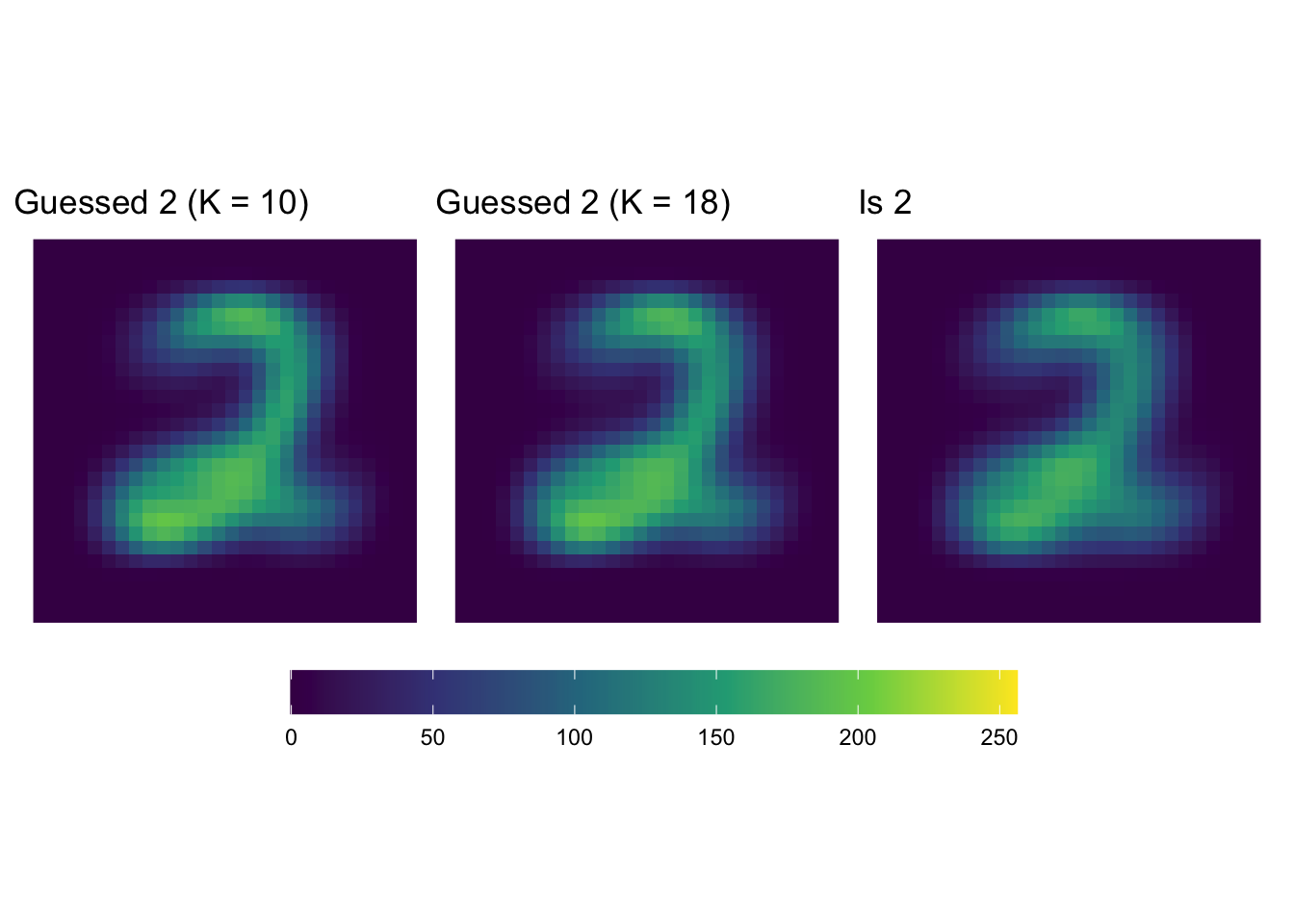
ggtitle("Guessed 2 (K = 18)")
(guess2 + ggtitle('Guessed 2 (K = 10)')) + guess2_18 + is2 +
plot_layout(guides = "collect") &
theme(
legend.position = "bottom",
legend.key.width = unit(2, "cm")
)
Question: Is cross validation important here? Why/why not?
PCA
K-means clustering is just one approach to unsupervised learning. As I hinted at in the in-class activity, another common method is principal component analysis (PCA).
The basic idea behind PCA is to find the reduce your feature (predictor) space to fewer dimensions that still account for a sizable amount of variation.
So you’re going to break your dataset up into “components”, each of which is a linear combination of your features (note the linearity). For example, the first principal component (with features \(X_{1}\) through \(X_{p}\)) is
\[Z_{1} = \phi_{11} X_{1} + \phi_{21} X_{2} + \cdots + \phi_{p1} X_{p}\] and the second principal component is
\[Z_{2} = \phi_{12} X_{1} + \phi_{22} X_{2} + \cdots + \phi_{p2} X_{p}\]
We choose the values of \(\phi_{ij}\) so that account for the largest amount of variance in the features—and we do it sequentially (think back to greedy splitting in trees). First we find \(\phi_{11}\) through \(\phi_{p1}\) to define the first principal component.
A few notes:
- PCA assumes/requires that the variables have been centered (demeaned). You probably want to scale those variables too.
- We normalize the \(\phi_{ij}\) so that the squared sum of “coefficients” for a given principal component sum to 1, i.e., for the first principal component, \(\sum_{j=1}^{p} \phi_{j1}^2 = 1\).
- Each principal component must be uncorrelated with previous principal components (think of it as previous components’ variation is already claimed).
- Subsequent components will explain less and less variation in the feature space. You’ll often see people sum the variance explained by several principal components to see how much of the variation they explain.
- The first principal component is the hyperplane ‘nearest’ to the points.
Mathematically, we end up deriving the principal components via eigenvalue decomposition—but we’ll leave that for your pleasure reading.
Nice visualization here (plus another resource).
# Add PCA to recipe
simple_recipe_pca =
  recipe(
    label ~ .,
    data = train_dt %>% select(label, starts_with('pixel'))
  ) %>%
  step_mutate(label = as.factor(label)) %>%
  step_center(all_numeric_predictors()) %>%
  step_pca(all_predictors(), threshold = 0.9) %>%
  step_rm(starts_with("pixel"))
# Calculate PCs
train_pc = simple_recipe_pca %>% prep() %>% juice()
Note: You should probably scale, but a few pixels cause issues.
We can repeat our K means clustering on the principal components that jointly contribute to 90% of the variance in the predictors (pixels).
find_k_pca = mclapply(
  mc.cores = parallel::detectCores(),
  X = 1:40,
  FUN = function(k) {
    # Try 'k' clusters
    k_centers = KMeans_arma(
      data = train_pc %>% select(starts_with('PC')),
      clusters = k
    )
    # Add cluster to the training dataset
    k_dt = data.table(
      label = train_pc$label,
      cl = predict_KMeans(
        data = train_pc %>% select(starts_with('PC')),
        CENTROIDS = k_centers
      )
    )
    # Find modal label for each cluster
    k_dt[, pred := collapse::fmode(label), cl]
    # Return a data table with accuracy
    data.table(
      k = k,
      accuracy = k_dt[,mean(label == pred)]
    )
  }
) %>% rbindlist()
And the performance…
ggplot(
  data = find_k_pca,
  aes(x = k, y = accuracy)
) +
geom_line(data = find_k, size = 1/4) +
geom_point(data = find_k, size = 2.5) +
geom_hline(yintercept = 0, size = 1/5) +
geom_line(size = 1/4, color = 'orange') +
geom_point(size = 2.5, color = 'orange', shape = 1) +
theme_minimal() +
scale_y_continuous('Accuracy', labels = scales::percent, limits = c(0, 1))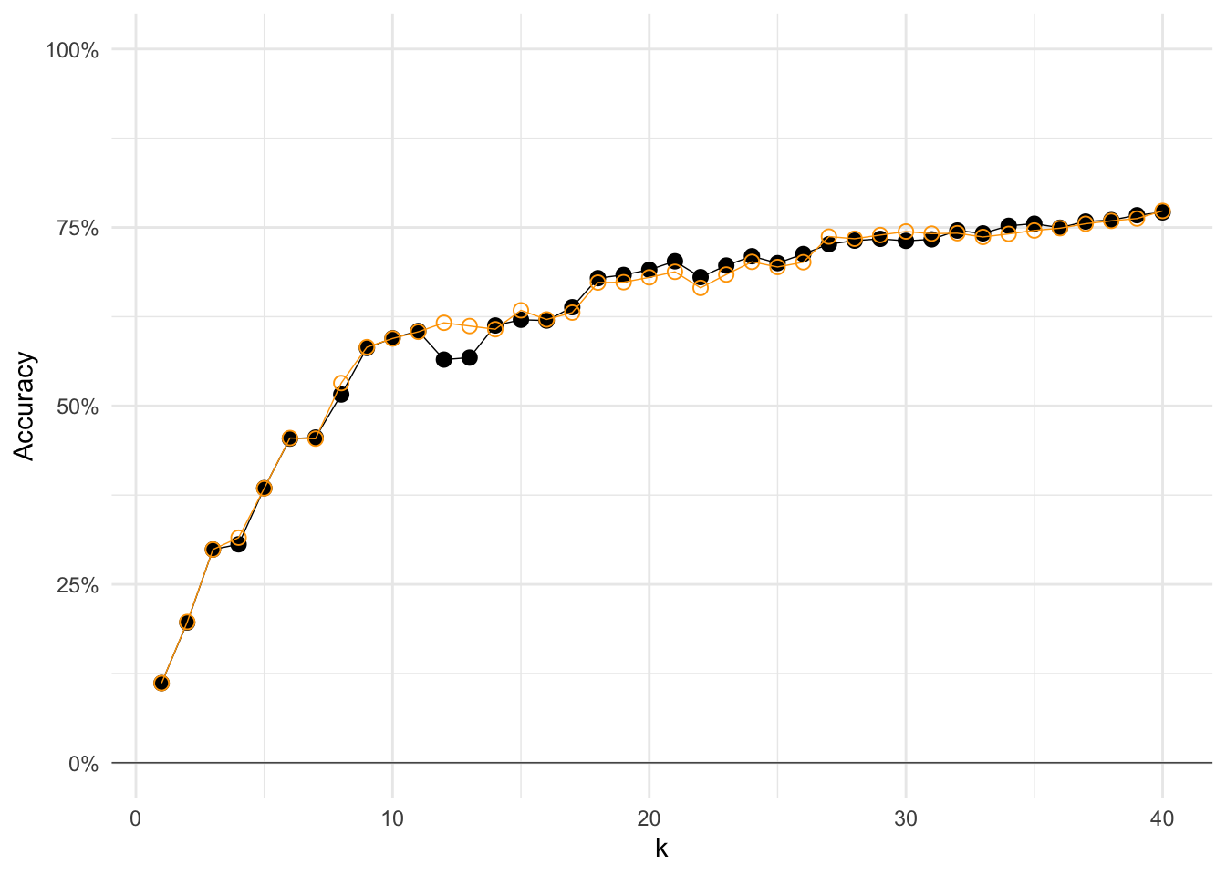
You might be thinking “they’re almost the same!” And you’re right. PCA is just taking linear combinations of the features (our pixels), and then K-means is looking for clusters in these linear combinations—rather than in the pixels themselves.
But the cool thing is that we are getting the same performance in a fraction of the dimensions. This new K-means algorithm only had to consider 4.1999^{4} dimensions, instead of the original 784.
There’s (always) more
Before we wrap up, let’s try one more dimensionality-reduction tool: UMAP. Specifically, UMAP (similar to t-SNE) gives us a nonlinear dimensionality reduction—essentially by trying to create a lower-dimensional representation of the original space. I’ll let you read about UMAP on your own, but here’s how you could do it with the embed package (extending tidymodels).
# Add PCA to recipe
simple_recipe_umap =
  recipe(
    label ~ .,
    data = train_dt %>% select(label, starts_with('pixel'))
  ) %>%
  step_mutate(label = as.factor(label)) %>%
  step_center(all_numeric_predictors()) %>%
  step_umap(all_predictors(), num_comp = 2) %>%
  step_rm(starts_with("pixel"))
# Calculate PCs
train_umap = simple_recipe_umap %>% prep() %>% juice()
Now apply K means on our greatly reduced dimensions!
find_k_umap = mclapply(
  mc.cores = parallel::detectCores(),
  X = 1:40,
  FUN = function(k) {
    # Try 'k' clusters
    k_centers = KMeans_arma(
      data = train_umap %>% select(starts_with('UMAP')),
      clusters = k
    )
    # Add cluster to the training dataset
    k_dt = data.table(
      label = train_umap$label,
      cl = predict_KMeans(
        data = train_umap %>% select(starts_with('UMAP')),
        CENTROIDS = k_centers
      )
    )
    # Find modal label for each cluster
    k_dt[, pred := collapse::fmode(label), cl]
    # Return a data table with accuracy
    data.table(
      k = k,
      accuracy = k_dt[,mean(label == pred)]
    )
  }
) %>% rbindlist()
And the performance…
ggplot(
  data = find_k_umap,
  aes(x = k, y = accuracy)
) +
geom_line(data = find_k, size = 1/4) +
geom_point(data = find_k, size = 2.5) +
geom_hline(yintercept = 0, size = 1/5) +
geom_line(data = find_k_pca, size = 1/4, color = 'orange') +
geom_point(data = find_k_pca, size = 2.5, color = 'orange', shape = 1) +
geom_line(size = 1/4, color = 'deeppink2') +
geom_point(size = 2.5, color = 'deeppink2', shape = 16) +
theme_minimal() +
scale_y_continuous('Accuracy', labels = scales::percent, limits = c(0, 1))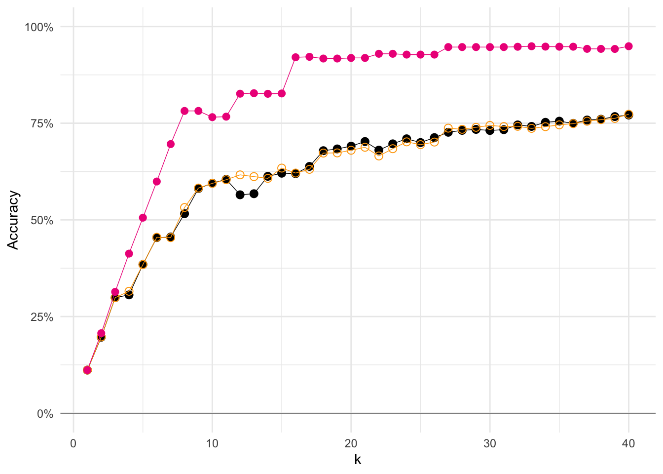
And that’s with only 2 dimensions! Pretty cool, right?
Note: It would probably still be good to validate our test performance properly.