Main references for today
- Miranda & Fackler (2002), Ch. 4
- Judd (1998), Ch. 4
- Nocedal & Writght (2006), Chs. 12, 15, 17–19
- Lecture notes from Ivan Rudik (Cornell) and Florian Oswald (SciencesPo)
- A.K. Dixit (1990), Optimization in Economic Theory
Constrained optimization: theory and methods
University of Illinois Urbana-Champaign
We want to solve
\[\min_x f(x)\]
subject to
\[ \begin{gather} g(x) = 0\\ h(x) \leq 0 \end{gather} \]
where \(f:\mathbb{R}^n \rightarrow \mathbb{R}\), \(g:\mathbb{R}^n \rightarrow \mathbb{R}^m\), \(h:\mathbb{R}^n \rightarrow \mathbb{R}^l\), and \(f, g\), and \(h\) are twice continuously differentiable
Constraints come in two types: equality or inequality
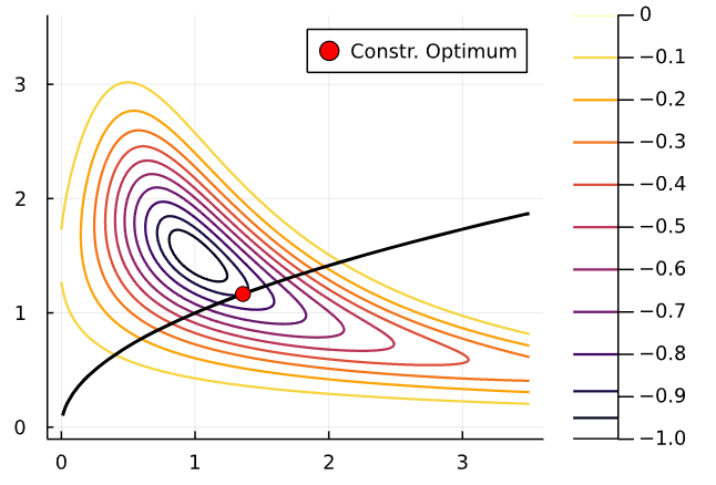
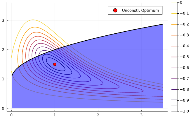
Let’s see a an illustration with a single constraint. Consider the optimization problem
\[ \min_x -exp\left(-(x_1 x_2 - 1.5)^2 - (x_2 - 1.5)^2 \right) \]
subject to \(x_1 - x_2^2 = 0\)
The problem can also be formulated with an inequality constraint
\[ \min_x -exp\left(-(x_1 x_2 - 1.5)^2 - (x_2 - 1.5)^2 \right) \]
subject to \(-x_1 + x_2^2 \leq 0\)
How would that change feasible set compared to the equality constraint?
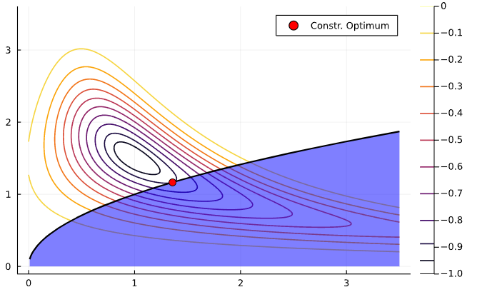
If the solution is interior to the feasible set, we say the constraint is slack or inactive
You may recall from Math Econ courses that, under certain conditions, we can solve a constrained optimization problem by solving instead the corresponding mixed complementary problem using the first order conditions
That trick follows from the Karush-Kuhn-Tucker (KKT) Theorem
What does it say?
If \(x^*\) is a local minimizer and the constraint qualification1 holds, then there are multipliers \(\lambda^* \in \mathbb{R}^m\) and \(\mu^* \in \mathbb{R}^l\) such that \(x^*\) is a stationary point of \(\mathcal{L}\), the Lagrangian
\[ \mathcal{L}(x, \lambda, \mu) = f(x) + \lambda^T g(x) + \mu^T h(x) \]
How does this theorem help us?
Put another way, the theorem states that \(\mathcal{L}_x(x^*, \lambda^*, \mu^*) = 0\)
So, it tell us that \((x^*, \lambda^*, \mu^*)\) solve the system
\[ \begin{gather} f_x + \lambda^T g_x + \mu^T h_x = 0 \\ \mu_i h^i(x) = 0, \; i = 1, \dots, l \\ g(x) = 0 \\ h(x) \leq 0 \\ \mu \leq 0 \end{gather} \]
The KKT theorem gives us a first approach to solving unconstrained optimization problems
Let \(\mathcal{I}\) be the set of \({1, 2, ..., l}\) inequality constraints. For a subset \(\mathcal{P} \in \mathcal{I}\), we define the \(\mathcal{P}\) problem as the nonlinear system of equations
\[ \begin{gather} f_x + \lambda^T g_x + \mu^T h_x = 0 \\ h^i(x) = 0, \; i \in \mathcal{P} \\ \mu_i = 0, \; i \in \mathcal{I} - \mathcal{P} \\ g(x) = 0 \end{gather} \]
We solve this system for every possible combination of binding constraints \(\mathcal{P}\)
The combinatorial nature of the KKT approach is not that desirable from a computational perspective
However, if the resulting nonlinear systems are simple to solve, we may still favor KKT
There are computational alternatives to KKT. We’ll discuss three types of algorithms
Suppose we wish to minimize some function subject to equality constraints (easily generalizes to inequality) \[ \min_x f(x) \,\,\, \text{s. t.} \,\, g(x) = 0 \]
How does an algorithm know to not violate the constraint?
One way is to introduce a penalty function into our objective and remove the constraint
\[ Q(x;\rho) = f(x) + \rho P(g(x)) \]
where \(\rho\) is the penalty parameter
With this, we transformed it into an unconstrained optimization problem \[ \min_x Q(x; \rho) = f(x) + \rho P(g(x)) \]
How do we pick \(P\) and \(\rho\)?
A first idea is to penalize a candidate solution as much as possible whenever it leaves the feasible set: infinite penalty!
\[Q(x) = f(x) + \infty \mathbf{1}(g(x) \neq 0)\] where \(\mathbf{1}\) is an indicator function
However, the infinite step method is a pretty bad idea
So we might instead use a more forgiving penalty function
A widely-used choice is the quadratic penalty function
\[Q(x;\rho) = f(x) + \frac{\rho}{2} \sum_i g_i^2(x)\]
The second term increases the value of the function
The penalty terms are smooth \(\rightarrow\) use unconstrained optimization techniques
to solve the problem by searching for iterates of \(x_k\)
Algorithms generally iterate on sequences of \(\rho_k \rightarrow \infty\) as \(k \rightarrow \infty\), to require satisfying the constraints as we close in
There are also Augmented Lagrangian methods that take the quadratic penalty method and add explicit estimates of Lagrange multipliers to help force binding constraints to bind precisely
Example: \[ \min x_1 + x_2 \,\,\,\,\,\text{ subject to: } \,\,\, x_1^2 + x_2^2 - 2 = 0 \]
Solution is pretty easy to show to be \((-1, -1)\)
The penalty method function \(Q(x_1, x_2; \rho)\) is
\[ Q(x_1, x_2; \rho) = x_1 + x_2 + \frac{\rho}{2} (x_1^2 + x_2^2 - 2)^2 \]
Let’s ramp up \(\rho\) and see what happens to how the function looks
\(\rho = 1\), solution is around \((-1.1, -1.1)\)
\(\rho = 10\), solution is very close to \((-1, -1)\). Notice how quickly value increases outside \(x_1^2 + x_2^2 = 2\) circle
The KKT method can lead to too many combinations of constraints to evaluate
Penalty methods don’t have the same problem but still require us to evaluate every constraint, even if they are not binding
Improving on the KKT approach, active set methods strategically pick a sequence of combinations of constraints
Instead of trying all possible combinations, like in KKT, active set methods start with an initial guess of the binding constraints set
Then, iterate by periodically checking constraints
If an appropriate strategy of picking sets is chosen, active set algorithms converge to the optimal solution
Interior point methods are also called barrier methods
Issue: how do we ensure we are on the interior of the feasible set?
Main idea: impose a barrier to stop the solver from letting a constraint bind
Consider the following constrained optimization problem
\[ \begin{gather} \min_{x} f(x) \notag\\ \text{subject to: } g(x) = 0, h(x) \leq 0 \end{gather} \]
Reformulate this problem as
\[ \begin{gather} \min_{x,s} f(x) \notag\\ \text{subject to: } g(x) = 0, h(x) + s = 0, s \geq 0 \end{gather} \]
where \(s\) is a vector of slack variables for the constraints
Final step: introduce a barrier function to eliminate the inequality constraint,
\[ \begin{gather} \min_{x,s} f(x) - \mu \sum_{i=1}^l log(s_i) \notag\\ \text{subject to: } g(x) = 0, h(x) + s = 0 \end{gather} \]
where \(\mu > 0\) is a barrier parameter
The barrier function prevents the components of \(s\) from approaching zero by imposing a logarithmic barrier \(\rightarrow\) it maintains slack in the constraints
Interior point methods solve a sequence of barrier problems until \(\mu_k\) converges to zero
The solution to the barrier problem converges to that of the original problem