ACE 592 - Lecture 3.3

Complementarity Problems

Diego S. Cardoso

University of Illinois Urbana-Champaign

Course Roadmap

1. Introduction to Scientific Computing
2. Fundamentals of numerical methods
3. Systems of equations
   1. Linear systems
   2. Nonlinear systems
   3. Complementarity problems
4. Optimization
5. Function approximation
6. Structural estimation

Agenda

• Today, we will cover complementarity problems, which are a generalization of rootfinding problems that allow for constraints on the solution
• Here, we cover how to set up and solve mixed complementarity problems in Julia

Main references

• Miranda & Fackler (2002), Chs. 3.7 and 3.8
• Lecture notes for Ivan Rudik’s Dynamic Optimization (Cornell)

Complementarity problems

In these problems, we have

• A function \(f: \mathbb{R}^n \rightarrow \mathbb{R}^n\)
• n-vectors \(a\) and \(b\), with \(a<b\)

And we are looking for an n-vector \(x \in [a,b]\) such that for all \(i = 1,\dots,n\)

\[ \begin{align*} x_i > a_i \Rightarrow f_i(x) \geq 0 \\ x_i < b_i \Rightarrow f_i(x) \leq 0 \end{align*} \]

• This formulation is usually referred to as a Mixed Complementarity Problem because it has an upper and lower bounds
  • Standard complementarity problems have one-sided bounds

Complementarity problems

An economic interpretation

• \(x\) is an n-dimensional vector of some economic action
• \(a_i\) and \(b_i\) are the lower and upper bounds on action \(i\)
• \(f_i(x)\) is the marginal arbitrage profit of action \(i\)

There are disequilibrium profit opportunities if

1. \(x_i < b_i\) and \(f_i(x) > 0\) (we can increase profits by raising \(x_i\))

2. \(x_i > a_i\) and \(f_i(x) < 0\) (we can increase profits by decreasing \(x_i\))

Complementarity problems

We obtain a no-arbitrage equilibrium if and only if \(x\) solves the complementary problem \(CP(f,a,b)\)

We can write out the problem as finding a vector \(x \in [a,b]\) that solves

\[ \begin{align} x_i > a_i \Rightarrow f_i(x) \geq 0 \,\,\, \forall i = 1,...,n \notag\\ x_i < b_i \Rightarrow f_i(x) \leq 0 \,\,\, \forall i = 1,...,n \notag \end{align} \]

At interior solution, the function must be precisely be zero

Corner solution at the upper bound \(b_i\) for \(x_i\) \(\rightarrow\) \(f\) must be increasing in direction \(i\)

The opposite is true if we are at the lower bound

Complementarity problems

Most economic problems are complementarity problems where we are

• Looking for a root of a function (e.g. marginal profit)
• Subject to some constraint (e.g. price floors)

The Karush-Kuhn-Tucker theorem shows that \(x\) solves the constrained optimization problem ( \(\max_x F(x)\) subject to \(x \in [a,b]\)) only if it solves the complementarity problem \(CP(f, a, b)\), where \(f_i = \partial F/\partial x_i\)

Let’s use a linear \(f\) to visualize what do we mean by a solution in complementarity problems

Complementarity problems

Case 1

What is the solution?

\(x^{*} = a\), with \(f(x^{*}) < 0\)

Another way of seeing it: imagine we’re trying to maximize \(F\)

What would \(F\) look like between \(a\) and \(b\)?

• The decreasing part of a concave parabola

Complementarity problems

Case 2

What is the solution?

\(x^{*} = b\), with \(f(x^{*}) > 0\)

Once again, imagine we’re trying to maximize \(F\)

What would \(F\) look like between \(a\) and \(b\)?

• The increasing part of a concave parabola

Complementarity problems

Case 3

What is the solution?

Some \(x^{*}\) between \(a\) and \(b\), with \(f(x^{*}) = 0\)

What would \(F\) look like between \(a\) and \(b\)?

• A concave parabola with an interior maximum

Complementarity problems

Case 4

What is the solution?

Actually, we have 3 solutions:

1. \(x^{*} = a\), with \(f(x^{*}) < 0\)
2. \(x^{*} = b\), with \(f(x^{*}) > 0\)
3. Some \(x^{*} \in (a,b)\), with \(f(x^{*}) = 0\)

• And this is an unstable solution

What would \(F\) look like between \(a\) and \(b\)?

• A convex parabola! So we end up with multiple local maxima that satisfy the 1st-order condition

Solving CPs

A complementarity problem \(CP(f, a, b)\) can be re-framed as a rootfinding problem

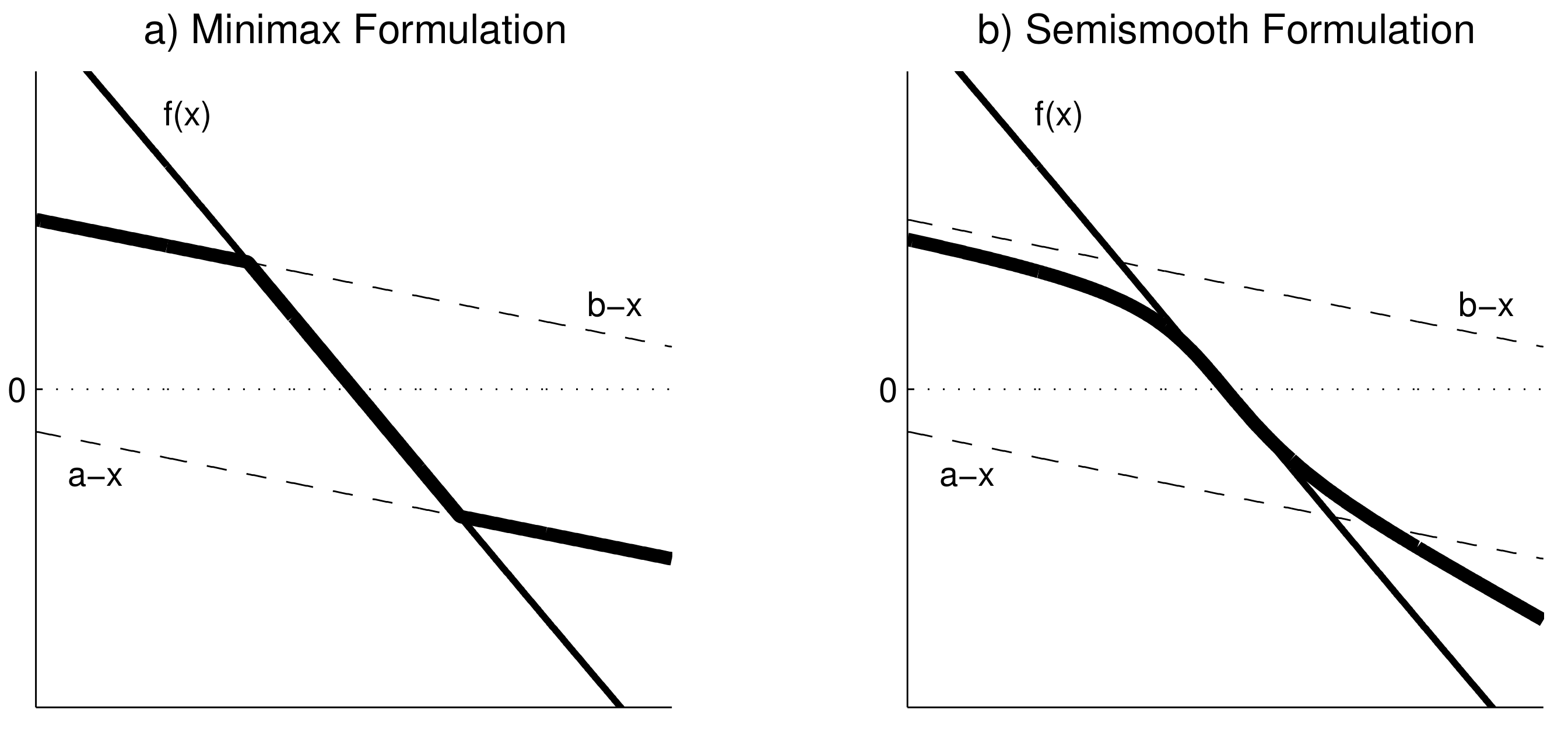
\[ \hat{f}(x) = min(max(f(x),a-x),b-x) = 0 \]

Let’s revisit those 4 cases to understand why this works

Solving CPs

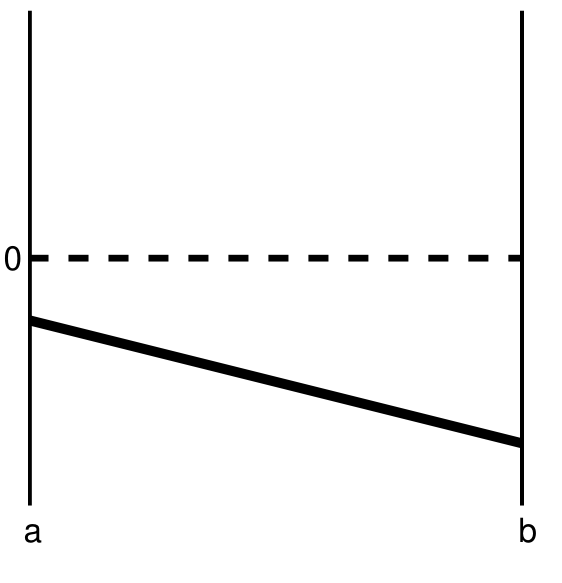
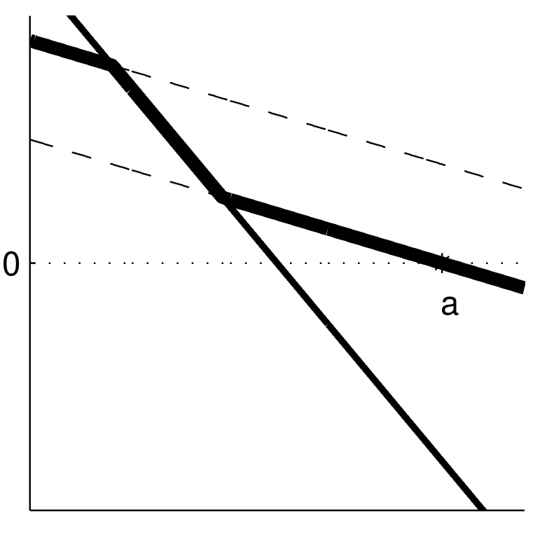
Case 1

\(\hat{f}(x) = min(max(f(x),a-x),b-x) = 0\)

• Dashed lines are \(b-x\) and \(a-x\)
• Thin solid line is \(f(x)\)
• Thick solid line is \(\hat{f}(x)\)

\(\rightarrow\) The solution is \(x^{*} = a\)

• Note that \(f(x) < 0\) for all \(x \in [a,b]\), so this is still case 1

Solving CPs

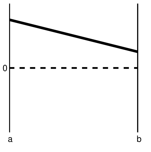
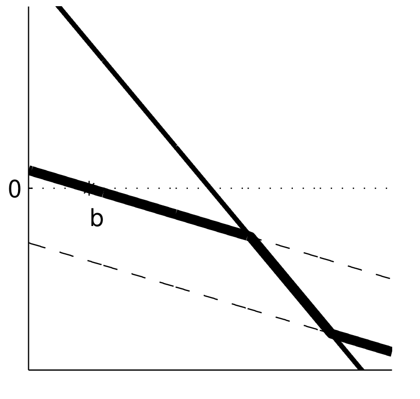
Case 2:

\(\hat{f}(x) = min(max(f(x),a-x),b-x) = 0\)

In this case, \(f(x) > 0\) for all \(x \in [a,b]\)

\(\rightarrow\) The solution is \(x^{*} = b\)

Solving CPs

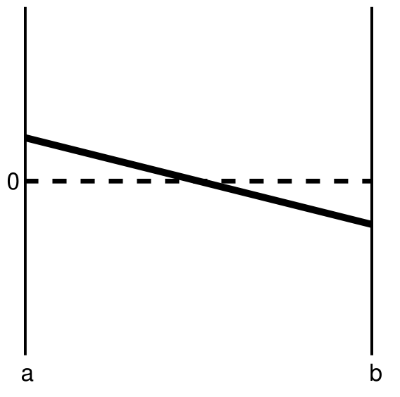
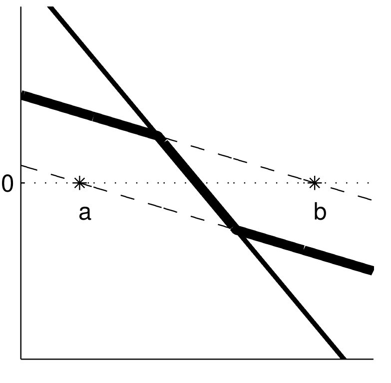
Case 3:

\(\hat{f}(x) = min(max(f(x),a-x),b-x) = 0\)

In this case, \(f(a) > 0\), \(f(b) < 0\)

\(\rightarrow\) The solution is some \(x^{*} \in (a, b)\)

Solving CPs

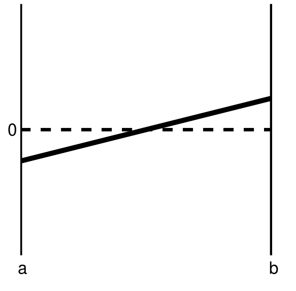
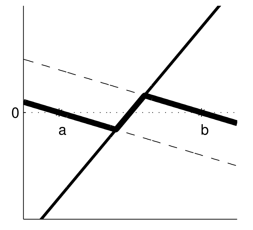
Case 4:

\(\hat{f}(x) = min(max(f(x),a-x),b-x) = 0\)

In this case, \(f(a) < 0\), \(f(b) > 0\)

\(\rightarrow\) We have the same 3 solutions

1. \(x^{*} = a\), with \(f(x^{*}) < 0\)
2. \(x^{*} = b\), with \(f(x^{*}) > 0\)
3. Some \(x^{*} \in (a,b)\), with \(f(x^{*}) = 0\)

Solving CPs

Once \(\hat{f}\) is defined, we can use Newton’s or quasi-Newton methods to solve a CP

If using Newton, we need to define the Jacobian \(\hat{J}(x)\) with row \(i\) being

• \(\hat{J}_i(x) = J_i(x)\), if \(a_i - x_i < f_i(x) < b_i - x_i\)
• \(\hat{J}_i(x) = -I_i(x)\), otherwise

where \(I\) is the identity matrix

Solving CPs

Rootfinding with \(\hat{f}\) works well in many cases but can be problematic in others

One problem is that \(\hat{f}\) has nondiferentiable kinks. This can lead to slower convergence, cycles, and incorrect answers¹

A workaround is to use an alternative function with smoother transitions, such as Fischer’s function

\[ \tilde{f}(x) = \phi^{-}(\phi^{+}(f(x), a-x), b-x) \]

where \(\phi_i^\pm(u, v) = u_i + v_i \pm \sqrt{u_i^2 + v_i^2}\)

1. See Miranda & Fackler (2002) Ch. 3.8 for a pathological example that needs smoothing.

Solving CPs

Solving CPs in Julia

We can use NLsolve.mcpsolve to solve CPs for us.¹ Let’s see an example of \(f:\mathbb{R}^2\rightarrow\mathbb{R}^2\)

\[ \begin{align*} f_1(x_1, x_2) & = 3x_1^2 + 2x_1x_2 + 2x_2^2 + 4x_1 - 2 \\ f_2(x_1, x_2) & = 2x_1^2 + 5x_1x_2 - x_2^2 + x_2 + 1 \end{align*} \]

function f!(F, x) # We need to program the memory-efficient version here
    F[1] = 3*x[1]^2 + 2*x[1]*x[2] + 2*x[2]^2 + 4*x[1] - 2
    F[2] = 2*x[1]^2 + 5*x[1]*x[2] -   x[2]^2 + x[2] + 1
end;

1. Because complementarity conditions are constraints, a more comprehensive way for larger systems is through JuMP.jl modeling interface. We will cover that in the Constrained Optimization unit.

Solving CPs in Julia

Let’s check the solution to the standard rootfinding problem using Newton’s method

using NLsolve;
NLsolve.nlsolve(f!, [1.0; 1.0], method=:newton)

Results of Nonlinear Solver Algorithm
 * Algorithm: Newton with line-search
 * Starting Point: [1.0, 1.0]
 * Zero: [-0.13736984903421828, 1.1872338075744588]
 * Inf-norm of residuals: 0.000000
 * Iterations: 7
 * Convergence: true
   * |x - x'| < 0.0e+00: false
   * |f(x)| < 1.0e-08: true
 * Function Calls (f): 8
 * Jacobian Calls (df/dx): 8

Solving CPs in Julia

Getting back to CPs, let’s impose non-negativity bounds on \(x_1\) and \(x_2\) but no upper bounds (i.e., \(b = \infty\))

a = [0.0; 0.0]; b = [Inf; Inf];
r = NLsolve.mcpsolve(f!, a, b, [1.0; 1.0], method=:newton, reformulation=:minmax)

Results of Nonlinear Solver Algorithm
 * Algorithm: Newton with line-search
 * Starting Point: [1.0, 1.0]
 * Zero: [0.3874258867227982, 0.0]
 * Inf-norm of residuals: 0.000000
 * Iterations: 10
 * Convergence: true
   * |x - x'| < 0.0e+00: false
   * |f(x)| < 1.0e-08: true
 * Function Calls (f): 17
 * Jacobian Calls (df/dx): 10

Solving CPs in Julia

We can get the value of the root using r.zero. Checking \(f(x^*)\)

r.zero

2-element Vector{Float64}:
 0.3874258867227982
 0.0

return_f = zeros(2);
f!(return_f, r.zero);
return_f

2-element Vector{Float64}:
 3.241851231905457e-14
 1.300197635405893

So the non-negativity constraint is binding for \(x_2\) but not \(x_1\)

Solving CPs in Julia

mcpsolve takes the same additional arguments nlsolve had: xtol, ftol, iterations, autodiff, show_trace, etc

In addition, it accepts argument reformulation, which can be smooth (default) or minmax

NLsolve.mcpsolve(f!, a, b, [1.0; 1.0], method=:newton, reformulation=:minmax, autodiff=:forward)

Results of Nonlinear Solver Algorithm
 * Algorithm: Newton with line-search
 * Starting Point: [1.0, 1.0]
 * Zero: [0.38742588672279815, 0.0]
 * Inf-norm of residuals: 0.000000
 * Iterations: 10
 * Convergence: true
   * |x - x'| < 0.0e+00: false
   * |f(x)| < 1.0e-08: true
 * Function Calls (f): 17
 * Jacobian Calls (df/dx): 10

Solving CPs in Julia

IMPORTANT NOTE. Miranda and Fackler’s textbook (and Matlab package) flip the sign convention for MCP problems. That’s because they are formulating it with an economic context in mind, where these problems arise from constrained optimization.

The conventional setup is (note the flipped inequalities)

\[ \begin{align*} x_i > a_i \Rightarrow f_i(x) \leq 0 \\ x_i < b_i \Rightarrow f_i(x) \geq 0 \end{align*} \]

Solution. If you are using standard MCP solvers (like mcpsolve), flip the sign of your \(f\) function

• For more details, see Miranda and Fackler’s Bibliographic Notes after Chapter 3

Example: Cournot duopoly with capacity constraints

Let’s revisit our duopoly example from Lecture 3.2 and add capacity constraints

Same setup as before:

• Inverse demand: \(P(Q) = \theta Q^{-1/\epsilon}\), where we add \(\theta\) as demand shifter
• Costs: \(C_i(q_i) = \frac{1}{2}c_i q_i^2\)

New: each firm has a capacity constraint \(q_i \in [0, K_i]\)

• Firm \(i\) maximizes \(\pi_i = P(Q)q_i - C_i(q_i)\) subject to \(0 \leq q_i \leq K_i\)

Example: Cournot duopoly as a CP

The KKT conditions for firm \(i\)’s problem are exactly the complementarity conditions

\[ \begin{align*} q_i > 0 &\Rightarrow \frac{\partial \pi_i}{\partial q_i} \leq 0 \\ q_i < K_i &\Rightarrow \frac{\partial \pi_i}{\partial q_i} \geq 0 \end{align*} \]

where marginal profit is

\[ f_i(q_1, q_2) = \theta Q^{-1/\epsilon} - \frac{\theta}{\epsilon} Q^{-1/\epsilon-1}q_i - c_i q_i \]

This is \(CP(f, a, b)\) with \(a = (0, 0)\) and \(b = (K_1, K_2)\)

Sign convention for mcpsolve

Recall that NLsolve.mcpsolve uses the convention

\[ \begin{align*} x_i > a_i &\Rightarrow f_i(x) \geq 0 \\ x_i < b_i &\Rightarrow f_i(x) \leq 0 \end{align*} \]

But our marginal profit \(f_i > 0\) means the firm wants to increase \(q_i\). At the upper bound \(q_i = K_i\), we expect \(f_i \geq 0\) (wants to produce more but can’t)

The KKT convention has the opposite sign: \(q_i < b_i \Rightarrow f_i \geq 0\), but mcpsolve expects \(f_i \leq 0\)

We need to pass \(-f\) to mcpsolve

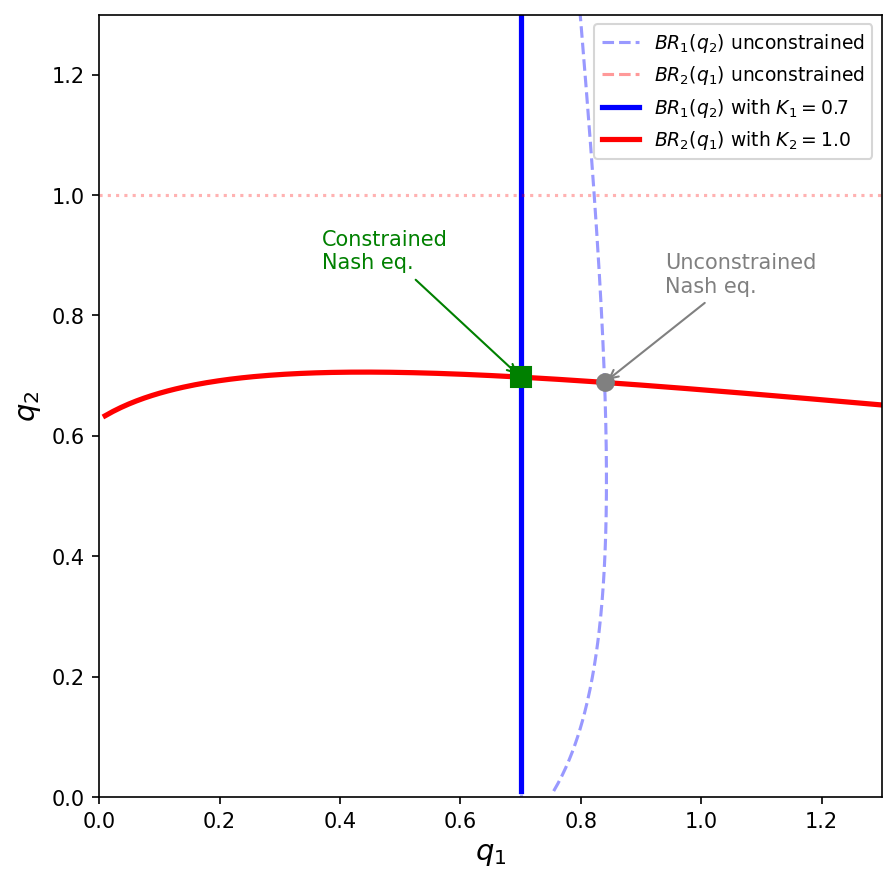
Example: best responses with capacity constraints

Without constraints, the Nash equilibrium is \((q_1^*, q_2^*) \approx (0.84, 0.69)\)

But firm 1 (the low-cost firm) can’t produce more than \(K_1 = 0.7\)!

The constrained equilibrium: \(q_1^* = 0.7\) (at capacity) and \(q_2^* \approx 0.70\) (interior)

• Firm 1’s marginal profit is positive at \(q_1 = K_1\): it would produce more if it could
• Firm 2’s marginal profit is zero: it is at its unconstrained optimum

This is precisely the complementarity structure: firm 1 is at the upper bound with \(f_1 > 0\), while firm 2 is interior with \(f_2 = 0\)

Example: defining the CP with NLsolve

We define the functions kind of like before, but now using a vector of parameters and flipping the sign convention

epsilon = 1.6; c = [0.6; 0.8]; theta = 1.0; K = [0.7; 1.0];

function neg_foc!(F, q)
    Q = sum(q)
    for i in 1:2
        # NOTE: we flip the sign of f_i to match mcpsolve's convention
        F[i] = -(theta * Q^(-1/epsilon) - (theta/epsilon) * Q^(-1/epsilon - 1) * q[i] - c[i] * q[i])
    end
end

neg_foc! (generic function with 1 method)

Example: solving the CP with NLsolve

using NLsolve
a = [0.0; 0.0]; b = K;
r = NLsolve.mcpsolve(neg_foc!, a, b, [0.2, 0.2], method=:newton, autodiff=:forward)

Results of Nonlinear Solver Algorithm
 * Algorithm: Newton with line-search
 * Starting Point: [0.2, 0.2]
 * Zero: [0.7000000005741004, 0.6976530167583798]
 * Inf-norm of residuals: 0.000000
 * Iterations: 5
 * Convergence: true
   * |x - x'| < 0.0e+00: false
   * |f(x)| < 1.0e-08: true
 * Function Calls (f): 6
 * Jacobian Calls (df/dx): 5

Interpreting the solution

Remember to re-flip the sign of \(f\) to match the KKT convention

F_check = zeros(2); # Create a vector to store the value of f at the solution
neg_foc!(F_check, r.zero); # Compute f at the solution
println("f(q*) = $(-F_check)")

f(q*) = [0.13727104736212875, -1.489608436600065e-11]

• \(q_1^* = K_1 = 0.7\) with \(f_1 > 0\): firm 1 is capacity-constrained. Marginal profit is positive: it wants to produce more but can’t
• \(q_2^* \approx 0.70 < K_2\) with \(f_2 \approx 0\): firm 2 is at its interior optimum

Compare with the unconstrained solution from Lecture 3.2: [0.8396, 0.6888]

Without the constraint, firm 1 would produce \(\approx 0.84 > K_1\)

Best responses with capacity constraints

With capacity constraints, best response functions become truncated

Demand shifts and capacity constraints

Now let’s ask: what happens to the equilibrium as demand increases?

We vary \(\theta\) from \(0.3\) to \(3.0\)

As \(\theta\) rises, both firms want to produce more. Three regimes emerge:

1. Both interior (\(\theta < 0.75\)): neither constraint binds, both FOCs hold with equality
2. Firm 1 at capacity (\(0.75 \leq \theta < 1.77\)): firm 1 maxes out first (lower cost \(\rightarrow\) higher desired output), firm 2 expands
3. Both at capacity (\(\theta \geq 1.77\)): demand is so high that both firms are constrained

Equilibrium locus

Tracing the equilibrium locus

using Plots

thetas = range(0.3, 3.0, length=100)
q1_path = Float64[]; q2_path = Float64[];
q_init = [0.3; 0.25]

for θ in thetas
    function neg_foc_theta!(F, q)
        Q = sum(q)
        for i in 1:2
            F[i] = -(θ * Q^(-1/epsilon) - (θ/epsilon) * Q^(-1/epsilon - 1) * q[i] - c[i] * q[i])
        end
    end
    r = NLsolve.mcpsolve(neg_foc_theta!, a, b, q_init, method=:newton, autodiff=:forward)
    push!(q1_path, r.zero[1])
    push!(q2_path, r.zero[2])
    q_init = r.zero  # warm start for next iteration
end

Tracing the equilibrium locus

plot(collect(thetas), q1_path, label="q₁*", lw=2,
     xlabel="θ (demand shifter)", ylabel="Equilibrium output")
plot!(collect(thetas), q2_path, label="q₂*", lw=2)
hline!([0.7], label="K₁", ls=:dash, color=:blue, alpha=0.5)
hline!([1.0], label="K₂", ls=:dash, color=:red, alpha=0.5)

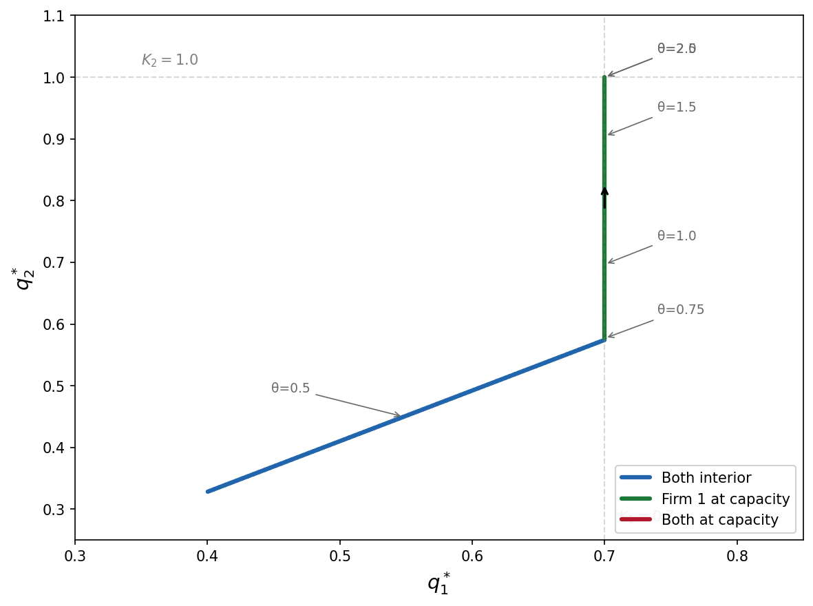
The kinks in the equilibrium paths correspond to transitions between regimes where different capacity constraints become binding

Takeaways from this example

1. CP conditions arise naturally from constrained optimization: the KKT conditions of the firms’ problems are exactly the CP conditions

2. Sign conventions matter: mcpsolve uses a different sign convention from the standard KKT formulation. Always check the documentation and verify the solution makes economic sense

3. The CP framework handles regime changes automatically: as \(\theta\) varies, the solver transitions between interior and corner solutions without us having to enumerate cases manually