We continue our study of methods to solve systems of equations, now looking at systems that contain nonlinear equations
Unlike linear systems, with nonlinear systems we don’t have guarantees of closed-form solutions, so solving them is harder
We will study two types of methods: derivative-free and derivative-based
Main references for today
Miranda & Fackler (2002), Ch. 3
Judd (1998), Ch. 5
Nocedal & Wright (2006), Ch. 11
Lecture notes for Ivan Rudik’s Dynamic Optimization (Cornell)
Types of nonlinear equation problems
Types of nonlinear equation problems
Problems involving nonlinear equations are very common in economics
We can classify them into two types
Systems of nonlinear equations
Complementarity problems
System of nonlinear equations
These come in two forms
Rootfinding problems
For a function \(f: \mathbb{R}^n \rightarrow \mathbb{R}^n\), we want to find a n-vector \(x\) that satisfies \(f(x) = 0\)
\(\rightarrow\) Any \(x\) that satisfies this condition is called a root of \(f\)
Examples?
Market equilibrium in general: market clearing conditions
No-arbitrage conditions (pricing models)
Solving first-order optimality conditions
System of nonlinear equations
Fixed-point problems
For a function \(g: \mathbb{R}^n \rightarrow \mathbb{R}^n\), we want to find a n-vector \(x\) that satisfies \(x = g(x)\)\(\rightarrow\) Any \(x\) that satisfies this condition is called a fixed point of \(g\)
Examples?
Best-response functions
Many equilibrium concepts in game theory
A Nash equilibrium is a fixed point in the strategy space
System of nonlinear equations
Rootfinding and fixed-point problems are equivalent
We can easily convert one into another
Rootfinding\(\rightarrow\)fixed-point
Define a new \(g(x) = x - f(x)\)
Fixed-point\(\rightarrow\)rootfinding
Define a new \(f(x) = x - g(x)\)
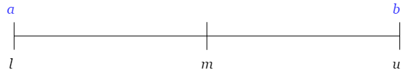
Complementarity problems
In these problems, we have
A function \(f: \mathbb{R}^n \rightarrow \mathbb{R}^n\)
n-vectors \(a\) and \(b\), with \(a<b\)
And we are looking for an n-vector \(x \in [a,b]\) such that for all \(i = 1,\dots,n\)
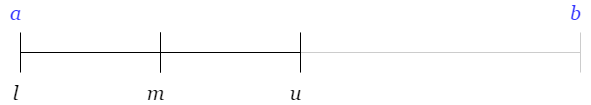
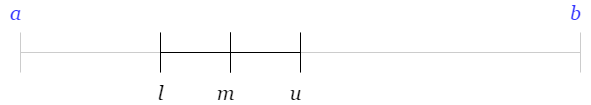
Repeat 2 and 3 until our interval is short enough ( \((u-l)/2 < tol\) ) and return \(x = m\)
Bisection method
Show the code
functionbisection(f, lo, up) tolerance =1e-3# tolerance for solution mid = (lo + up)/2# initial guess, bisect the interval difference = (up - lo)/2# initialize bound differencewhile difference > tolerance # loop until convergenceprintln("Intermediate guess: $mid")ifsign(f(lo)) ==sign(f(mid)) # if the guess has the same sign as the lower bound lo = mid # a solution is in the upper half of the interval mid = (lo + up)/2else# else the solution is in the lower half of the interval up = mid mid = (lo + up)/2end difference = (up - lo)/2# update the difference endprintln("The root of f(x) is $mid")end;
So it’s a good idea to check if you have the right boundaries
f(2.0)
0.75
f(4.0)
2.9375
These are both positive. So by the IVT, we can’t know for sure if there’s a root here
Bisection method
The bisection method is incredibly robust: if a function \(f\) satisfies the IVT, it is guaranteed to converge in a finite number of iterations
A root can be calculated to arbitrary precision \(\epsilon\) in a maximum of \(log_2\frac{b-a}{\epsilon}\) iterations
But robustness comes with drawbacks:
It only works in one dimension
It is slow because it only uses information about the function’s level but not its variation
Function iteration
For the next method, we recast rootfinding as a fixed-point problem
\[
f(x) = 0 \Rightarrow g(x) = x - f(x)
\]
Then, we start with an initial guess \(x^{(0)}\) and iterate \(x^{(k+1)}\leftarrow g(x^{k})\) until convergence: \(|x^{(k+1)}-x^{(k)}| \approx 0\)
Let’s try it!
Write a function that takes (f, initial_guess) and returns a root of \(f\) using function iteration
Then, use it to find the root of \(f(x) = -x^{-2} + x - 1\) with initial_guess = 1
Function iteration
Show the code
functionfunction_iteration(f, initial_guess) tolerance =1e-3# tolerance for solution difference =Inf# initialize difference x = initial_guess # initialize current valuewhileabs(difference) > tolerance # loop until convergenceprintln("Intermediate guess: $x") x_prev = x # store previous value x = x_prev -f(x_prev) # calculate next guess difference = x - x_prev # update differenceendprintln("The root of f(x) is $x")end;
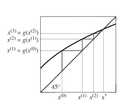
A fixed point \(x = g(x)\) is at the intersection between \(g(x)\) and the 45o line
Starting from \(x^{(0)}\), we calculate \(g(x^{(0)})\) and find the corresponding point on the 45o line for \(x^{(1)}\)
We keep iterating until we (approximately) find the fixed point
Function iteration
Function iteration is guaranteed to converge to a fixed point \(x^*\) if
\(g\) is differentiable, and
the initial guess is “sufficiently close” to an \(x^*\) at which \(\|g^\prime (x^{*}) \| < 1\)
It may also converge when these conditions are not met
Since this is an easy method to implement, it’s worth trying it before switching to more complex methods
Function iteration
But wait: What is “sufficiently close”?
Good question! There is no practical formula. As Miranda and Fackler (2002) put it
Typically, an analyst makes a reasonable guess for the root \(f\) and counts his/her blessings if the iterates converge. If the iterates do not converge, then the analyst must look more closely at the properties of \(f\) to find a better starting value, or change to another rootfinding method.
This is where science also becomes a bit of an art
Derivative-based methods
Newton’s method
Newton’s method and variants are the workhorses of solving n-dimensional non-linear problems
Key idea: take a hard non-linear problem and replace it with a sequence of linear problems \(\rightarrow\)successive linearization
Newton’s method
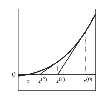
Start with an initial guess of the root at \(x^{(0)}\)
Approximate the non-linear function with its first-order Taylor expansion around \(x^{(0)}\)
This is just the tangent line at \(x^0\)
Solve for the root of this linear approximation, call it \(x^{(1)}\)
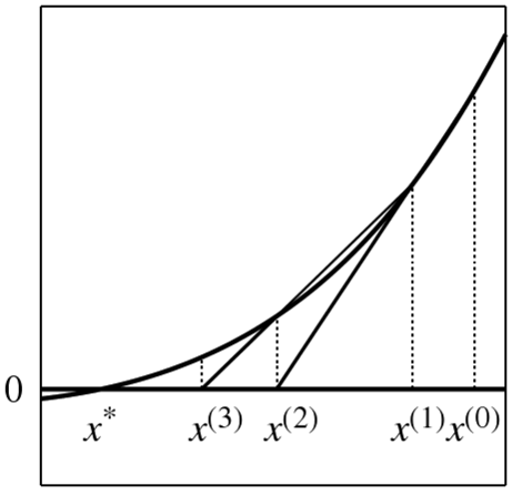
Newton’s method
Repeat starting at \(x^{(1)}\) until we converge to \(x^*\)
This can be applied to a function with an arbitrary number of dimensions
Newton’s method
Formally: begin with some initial guess of the root vector \(\mathbf{x^{(0)}}\)
Given \(\mathbf{x^{(k)}}\), our new guess \(\mathbf{x^{(k+1)}}\) is obtained by approximating \(f(\mathbf{x})\) using a first-order Taylor expansion around \(\mathbf{x^{(k)}}\)
functionnewtons_method(f, f_prime, initial_guess) tolerance =1e-3# tolerance for solution difference =Inf# initialize difference x = initial_guess # initialize current valuewhileabs(difference) > tolerance # loop until convergenceprintln("Intermediate guess: $x") x_prev = x # store previous value x = x_prev -f(x_prev)/f_prime(x_prev) # calculate next guess# ^ this is the only line that changes from function iteration difference = x - x_prev # update differenceendprintln("The root of f(x) is $x")end;
Newton’s method
f(x) =-x^(-2) + x -1;f_prime(x) =2x^(-3) +1;newtons_method(f, f_prime, 1.0)
Intermediate guess: 1.0
Intermediate guess: 1.3333333333333333
Intermediate guess: 1.4576271186440677
Intermediate guess: 1.4655459327062879
The root of f(x) is 1.465571231622256
Newton’s method
Newton’s method has nice properties regarding convergence and speed
It converges if
If \(f(x)\) is continuously differentiable,
The initial guess is “sufficiently close” to the root, and
\(f(x)\) is invertible near the root
We need \(f(x)\) to be invertible so the algorithm above is well defined
If \(f'(x)\) is ill-conditioned we can run into problems with rounding error
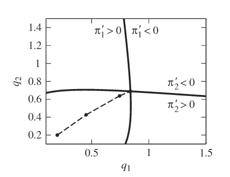
Newton’s method: a duopoly example
Inverse demand: \(P(q) = q^{-1/\epsilon}\)
Two firms with costs: \(C_i(q_i) = \frac{1}{2}c_i q_i^2\)
Visually, this is the path Newton’s method followed
Newton’s method: analytic vs numerical derivatives
It was tedious but in the previous example we could calculate the Jacobian analytically. Sometimes it’s much harder and we can make mistakes.
Here is a challenge for you: redo the previous example but, instead of defining the Jacobian analytically, use the ForwardDiff package to do the derivatives for you. Then, compare your solution with mine.
An alternative is to use the Symbolics.jl package. For low-dimensional derivative and Jacobians, it does a good job!
Quasi-Newton methods
We usually don’t want to deal with analytic derivatives unless we have access to autodifferentiation
Why?
It can be difficult to do the analytic derivation
Coding a complicate Jacobian is prone to errors and takes time
Can actually be slower to evaluate than finite differences for a nonlinear problem
Alternative \(\rightarrow\)finite differences instead of analytic derivatives
Quasi-Newton: Secant method
Using our current root guess \(x^{(k)}\) and our previous root guess \(x^{(k-1)}\):
We must initially provide a guess of the root, \(x^{(0)}\), but also a guess of the Jacobian, \(A_{(0)}\)
A good guess for \(A_{(0)}\) is to calculate it numerically at our chosen \(x^{(0)}\)
Quasi-Newton: Broyden’s method
The iteration rule is the same as before but with our guess of the Jacobian substituted in for the actual Jacobian (or the finite difference approximation)
Any reasonable guess for the Jacobian should satisfy this condition
But this gives \(n\) conditions with \(n^2\) elements to solve for in \(A\)
Quasi-Newton: Broyden’s method
Broyden’s methods solves this under-determined problem with an assumption that focuses on the direction we are most interested in: \(d^{(k)} = \mathbf{x^{(k+1)}} - \mathbf{x^{(k)}}\)
For any direction \(q\) orthogonal to \(d^{(k)}\), it assumes that \(A^{(k+1)}q = A^{(k)}q\)
In other words, our next guess is as good as the current ones for any changes in \(x\) that are orthogonal to the one we are interested right now
Jointly, the secant condition and the orthogonality assumption give the iteration rule for the Jacobian:
Before we continue, take a look again at our \(f\)
functionf(q) Q =sum(q) F = Q^(-1/epsilon) .- (1/epsilon)Q^(-1/epsilon-1) .*q .- c .*qend;
Do you see any potential inefficiency?
We allocate a new F every time we call this function!
Instead, we can be more efficient by writing a function that modifies a pre-allocated vector
Quick detour: functions that modify arguments
By convention, in Julia we name functions that modify arguments with a ! at the end. For our \(f\), we can define
functionf!(F, q) F[1] =sum(q)^(-1/epsilon) - (1/epsilon)sum(q)^(-1/epsilon-1)*q[1] - c[1]*q[1] F[2] =sum(q)^(-1/epsilon) - (1/epsilon)sum(q)^(-1/epsilon-1)*q[2] - c[2]*q[2]end;F =zeros(2) # This allocates a 2-vector with elements equal to zerof!(F, [0.2; 0.2]); # Note the first argument is a pre-allocated vectorF
Rootfinding algorithms will converge at different speeds in terms of the number of operations
A sequence of iterates \(x^{(k)}\) is said to converge to \(x^*\) at a rate of order \(p\) if there is a constant \(C\) such that
\[
\|x^{(k+1)}-x^{*}\|\leq C \|x^{(k)} - x^{*}\|^p
\]
for sufficiently large \(k\)
Convergence speed
\[
\|x^{(k+1)}-x^{*}\|\leq C \|x^{(k)} - x^{*}\|^p
\]
If \(C < 1\) and \(p = 1\): linear convergence
If \(1 < p < 2\): superlinear convergence
If \(p = 2\): quadratic convergence
The higher order the convergence rate, the faster it converges
Convergence speed
How fast do the methods we’ve seen converge?
Bisection: linear rate with \(C = 0.5\)
Function iteration: linear rate with \(C = ||f'(x^*)||\)
Secant and Broyden: superlinear rate with \(p \approx 1.62\)
Newton: \(p = 2\)
Convergence speed
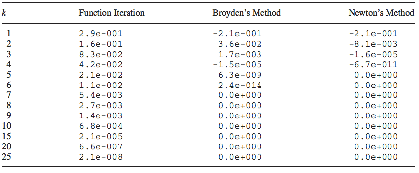
Consider an example where \(f(x) = x - \sqrt(x) = 0\)
This is how the 3 main approaches converge in terms of the \(L^1-\)norm for an initial guess \(x^{(0)} = 0.5\)
Choosing a solution method
Convergence rates only account for the number of iterations of the method
The steps taken in a given iteration of each solution method may vary in computational cost because of differences in the number of arithmetic operations
Although an algorithm may take more iterations to solve, each iteration may be solved faster and the overall algorithm takes less time
Choosing a solution method
Bisection method only requires a single function evaluation during each iteration
Function iteration only requires a single function evaluation during each iteration
Broyden’s method requires both a function evaluation and matrix multiplication
Newton’s method requires a function evaluation, a derivative evaluation, and solving a linear system
\(\rightarrow\) Bisection and function iteration are usually slow
\(\rightarrow\) Broyden’s method can be faster than Newton’s method if derivatives are costly to compute
Choosing a solution method
Besides convergence rates and algorithm speed, you should also factor development time
Newton’s method is fastest to converge
If deriving and programming the Jacobian is relatively simple and not too costly to compute, this method is a good choice
If derivatives are complex, quasi-Newton methods are good candidates
Bisection and function iteration are generally dominated options but are easy to program/debug, so they have value as a quick proof-of-concept
Bisection is often used in hybrid methods, such as Dekker’s and Brent’s. Hybrid methods select between bisection, secant, or other basic solution methods every iteration depending on a set of criteria
Common problems and solutions
When solvers fail: domain errors
A very common problem with Newton and Broyden: the solver tries values outside the function’s domain
Consider a market equilibrium with isoelastic supply \(S_i = c_i p_i^{\sigma_i}\) and demand \(D_i = y\, p_i^{\epsilon_{ii}} p_j^{\epsilon_{ij}}\)
# From an asymmetric guess, it crashes:try NLsolve.nlsolve(f!, [0.05; 2.0], method=:broyden)catcheprintln("Error: $e")end
Error: DomainError(-3.57491732087526, "Exponentiation yielding a complex result requires a complex argument.\nReplace x^y with (x+0im)^y, Complex(x)^y, or similar.")
What happened? Broyden’s approximate Jacobian led to a step that pushed \(p_1\) below zero. Julia tried to compute a negative number raised to a fractional power and threw a DomainError
Why this happens
Newton and Broyden are unconstrained methods: they search over all of \(\mathbb{R}^n\)
This is problematic when:
Variables must be positive (prices, quantities, income)
You use isoelastic functions: \(x^{\alpha}\) with non-integer \(\alpha\) requires \(x > 0\)
Your initial guess is far from the solution \(\rightarrow\) large steps \(\rightarrow\) overshooting
Broyden is more prone to this than Newton because its Jacobian approximation can degrade, leading to poorly directed steps
Three common strategies to deal with this:
Start with a better initial guess
Try a different method
Transform variables so the solver’s domain is unrestricted
Strategy 1: Better initial guesses
Idea: Solve a simpler version of the problem first, then use that solution as the starting point
For a system with cross-price effects, we can ignore them and solve each market in isolation
This has a closed-form solution and gives a reasonable starting point for the coupled system
Strategy 1: Better initial guesses
# Solve each market in isolation (set cross-price elasticities to zero)p0 = [(y₀/c[i])^(1/(σ[i] - ϵ_own[i])) for i in1:2];println("Simplified guess: $p0");
This is the same system, parameterized differently
Same equilibrium: if \(z^*\) solves \(g = 0\), then \(p^* = e^{z^*}\) solves \(f = 0\)
But now the solver can explore any \(z \in \mathbb{R}^2\) without ever triggering a domain error
Strategy 3: Variable transformation
functiong!(G, z) G[1] = c[1]*exp(σ[1]*z[1]) -y₀*exp(ϵ_own[1]*z[1] + ϵ_cross[1]*z[2]) G[2] = c[2]*exp(σ[2]*z[2]) -y₀*exp(ϵ_cross[2]*z[1] + ϵ_own[2]*z[2])end# Same starting point that failed before: p = (0.05, 2.0) → z = log.((0.05, 2.0))result = NLsolve.nlsolve(g!, log.([0.05; 2.0]), method=:broyden)p_solution =exp.(result.zero)println("Solution: p = $p_solution")
Solution: p = [1.877722541843727, 1.5818822321046384]
No DomainError. The solver explored negative \(z\) values, and \(e^z\) kept prices positive throughout
When to use each strategy
Better initial guess: simple, requires no code changes to \(f\), but needs problem-specific insight
Different method: Newton with autodiff is more robust than Broyden with finite differences, at the cost of more computation per step
Log transformation: most robust, works from distant guesses, but adds a layer of indirection and can lead to scaling issues if the solution is very large/small
Note: A related transformation for variables in \((0,1)\) (e.g., probabilities or shares):
\[
z = \log\!\left(\frac{x}{1-x}\right), \quad x = \frac{1}{1+e^{-z}}
\]
This is the logit transformation: \(z \in \mathbb{R}\) maps to \(x \in (0,1)\)
When solvers fail: convergence problems
We’ve seen that Newton’s method converges if the initial guess is sufficiently close to a root where \(f'\) is invertible
But what does failure look like in practice?
Three classic failure modes:
Cycling: iterates bounce back and forth without approaching the root
Divergence: iterates move farther and farther from the root
Slow convergence: iterates approach the root, but VERY slowly
The method enters a perfect 2-cycle: the tangent at \(x = 0\) hits zero at \(x = 1\), and the tangent at \(x = 1\) hits zero at \(x = 0\)
The actual root is at \(x^* \approx -1.77\), which Newton never reaches from this starting point
Failure mode 1: Cycling
Let’s verify with a modified version of our newtons_method function
f(x) = x^3-2*x +2;f_prime(x) =3*x^2-2;
We need to add a maximum iteration count so the loop terminates
functionnewtons_method_maxiter(f, f_prime, initial_guess; maxiter=20) tolerance =1e-3# tolerance for solution difference =Inf# initialize difference x = initial_guess # initialize current valuefor k in1:maxiterprintln("Iteration $k: x = $(round(x, digits=6))") x_prev = x x = x_prev -f(x_prev)/f_prime(x_prev) difference = x - x_prevabs(difference) < tolerance &&return xendprintln("Did not converge after $maxiter iterations")return xend;
Failure mode 1: Cycling
The iterates alternate between 0.0 and 1.0 indefinitely
Iteration 1: x = 0.0
Iteration 2: x = 1.0
Iteration 3: x = 0.0
Iteration 4: x = 1.0
Iteration 5: x = 0.0
Iteration 6: x = 1.0
Iteration 7: x = 0.0
Iteration 8: x = 1.0
Iteration 9: x = 0.0
Iteration 10: x = 1.0
Did not converge after 10 iterations
Failure mode 1: Cycling
Show the code
usingPlots; gr()f(x) = x^3-2*x +2;f_prime(x) =3*x^2-2;xgrid =range(-2.5, 2.0, length=300)p =plot(xgrid, f.(xgrid), label="f(x) = x³ - 2x + 2", color=:black, linewidth=2)hline!([0], color=:gray, linestyle=:dash, label=nothing)# Newton steps: tangent from (0, f(0)) to (1, 0), then (1, f(1)) to (0, 0)xs_cycle = [0.0, 1.0, 0.0, 1.0, 0.0]colors_cycle = [:royalblue, :crimson]for k in1:4 xk = xs_cycle[k]; xk1 = xs_cycle[k+1]plot!([xk, xk1], [f(xk), 0.0], color=colors_cycle[mod1(k,2)], linestyle=:dot, linewidth=1.5, label=nothing)plot!([xk1, xk1], [0.0, f(xk1)], color=colors_cycle[mod1(k,2)], linestyle=:dot, linewidth=1.5, label=nothing)endscatter!([0.0, 1.0], [f(0.0), f(1.0)], color=:red, markersize=6, label="Iterates")title!("Cycling: Newton bounces between x = 0 and x = 1")xlabel!("x"); ylabel!("f(x)")p
Failure mode 2: Divergence
Consider \(f(x) = \text{sign}(x)|x|^{1/3}\) (the cube root)
The root is at \(x^* = 0\), with \(f'(x) = \frac{1}{3}|x|^{-2/3}\). The Newton update simplifies to:
Iteration 1: x = 0.5
Iteration 2: x = -1.0
Iteration 3: x = 2.0
Iteration 4: x = -4.0
Iteration 5: x = 8.0
Iteration 6: x = -16.0
Iteration 7: x = 32.0
Iteration 8: x = -64.0
Did not converge after 8 iterations
Iteration 1: x = 1.0
Iteration 2: x = 0.666667
Iteration 3: x = 0.444444
Iteration 4: x = 0.296296
Iteration 5: x = 0.197531
Iteration 6: x = 0.131687
Iteration 7: x = 0.087791
Iteration 8: x = 0.058528
Iteration 9: x = 0.039018
Iteration 10: x = 0.026012
Iteration 11: x = 0.017342
Iteration 12: x = 0.011561
Iteration 13: x = 0.007707
Iteration 14: x = 0.005138
Iteration 15: x = 0.003425
Iteration 16: x = 0.002284
Failure mode 3: Slow convergence
Compare with a well-behaved case: \(f(x) = x^3 - 1\) has a simple root at \(x^* = 1\)
Show the code
# Collect errors for x^3 (repeated root)f_slow(x) = x^3; fp_slow(x) =3*x^2;x =1.0; errors_slow = [abs(x)]for k in1:50 x = x -f_slow(x)/fp_slow(x)push!(errors_slow, abs(x))end# Collect errors for x^3 - 1 (simple root)f_fast(x) = x^3-1; fp_fast(x) =3*x^2;x =2.0; errors_fast = [abs(x -1.0)]for k in1:15 x = x -f_fast(x)/fp_fast(x)push!(errors_fast, abs(x -1.0))endp =plot(0:length(errors_slow)-1, errors_slow, marker=:circle, markersize=3, color=:crimson, label="x³ (repeated root, linear rate)", yscale=:log10, xlabel="Iteration", ylabel="Error (log scale)", ylims=(1e-16, 10), linewidth=1.5)plot!(0:length(errors_fast)-1, errors_fast, marker=:diamond, markersize=3, color=:royalblue, label="x³ - 1 (simple root, quadratic rate)", linewidth=1.5)title!("Convergence comparison: repeated vs simple root")p
Failure mode 3: Slow convergence
The simple root reaches machine precision in about 7 iterations
The repeated root (level and 1st derivative) is still crawling after 50 iterations. Why?