3-element Vector{Float64}:
 -1.0
  2.0
1.0Main references for today
- Miranda & Fackler (2002), Ch. 2
- Judd (1998), Ch. 3
- Lecture notes for Ivan Rudik’s Dynamic Optimization (Cornell)
Linear Systems of Equations
University of Illinois Urbana-Champaign
(Systems of) Linear equations are very common in Economics
\[Ax = b\] where \(A\) is a \(n \times n\) matrix, \(b\) and \(x\) are \(n\)-vectors
Examples?
Solving linear systems is generally very easy in programming languages
3-element Vector{Float64}:
-1.0
2.0
1.0OK, so how does the computer actually solve linear equations?
Methods come in two flavors:
Let’s start with the simplest case: a lower triangular matrix
\[ A = \begin{bmatrix} a_{11} & 0 & 0 & \cdots & 0 \\ a_{21} & a_{22} & 0 & \cdots & 0 \\ a_{31} & a_{32} & a_{33} & \cdots & 0 \\ \vdots & \vdots & \vdots & \ddots & \vdots \\ a_{n1} & a_{n2} & a_{n3} & \cdots & a_{nn} \\ \end{bmatrix} , x = \begin{bmatrix} x_1 \\ x_2 \\ x_3 \\ \vdots \\ x_n \end{bmatrix} , b = \begin{bmatrix} b_1 \\ b_2 \\ b_3 \\ \vdots \\ b_n \end{bmatrix} \] How do we solve this?
Easy, forward substitution!
\[ \begin{align} x_1 = & b_1/a_{11} \\ x_2 = & (b_2 - a_{21}x_1)/a_{22} \\ x_3 = & (b_3 - a_{31}x_1 - a_{32}x_2)/a_{33} \\ \vdots \\ x_n = & (b_n - a_{n1}x_1 - a_{n2}x_2 - \cdots)/a_{nn} \\ \end{align} \]
We can write a simple algorithm to solve it: \(x_i=\left(b_i-\sum^{i-1}_{j=1} a_{ij}x_{j}\right)/a_{ii}\) for all \(i\)
What if \(A\) is upper triangular? We use backward substitution and just reverse the order
What is the complexity of this algorithm (in \(O\) notation)?
\(x_i=\left(b_i-\sum^{i-1}_{j=1} a_{ij}x_{j}\right)/a_{ii}\) for all \(i\)
What is the complexity of this algorithm?
There are:
Order of \(n^2/2\) operations \(\rightarrow O(n^2)\)
In practice we rarely need to solve triangular systems! What if \(A\) is not triangular?
This works for any non-singular matrix
This uses the fact that we can do the following operations to a linear system without changing its solution
We’ll use that to turn a matrix \((IA)\) into \((LU)\)
Let’s see an example with system \(Ax = b\)
\[ A = \begin{bmatrix} -3 & 2 & 3 \\ -3 & 2 & 1 \\ 3 & 0 & 0 \\ \end{bmatrix} , x = \begin{bmatrix} x_1 \\ x_2 \\ x_3 \\ \end{bmatrix} , b = \begin{bmatrix} 10 \\ 8 \\ -3 \\ \end{bmatrix} \]
We start with \(I = L, A = U\) and we to make \(U\) upper triangular with Gaussian elimination
\[ A = \begin{bmatrix} 1 & 0 & 0 \\ 0 & 1 & 0 \\ 0 & 0 & 1 \\ \end{bmatrix} \times \begin{bmatrix} -3 & 2 & 3 \\ -3 & 2 & 1 \\ 3 & 0 & 0 \\ \end{bmatrix} \] We do \(row2 = row2 - (1)\times row1\) and \(row3 = row3 - (-1)\times row1\), keeping track of these operations in the \(L\) matrix
\[ A = \begin{bmatrix} 1 & 0 & 0 \\ 1 & 1 & 0 \\ -1 & 0 & 1 \\ \end{bmatrix} \times \begin{bmatrix} -3 & 2 & 3 \\ 0 & 0 & -2 \\ 0 & 2 & 3 \\ \end{bmatrix} \]
Seems like we are stuck in \(U\). But we can swap rows 2 and 3 to make it upper triangular.
\[ A = \begin{bmatrix} 1 & 0 & 0 \\ 1 & 0 & 1 \\ -1 & 1 & 0 \\ \end{bmatrix}\times \begin{bmatrix} -3 & 2 & 3 \\ 0 & 2 & 3 \\ 0 & 0 & -2 \\ \end{bmatrix} \]
Now we are ready to solve the first part of the problem: \(Ly = b\)
But wait, \(L\) is not lower triangular!
Not yet. But all we need is for it to be row-permuted lower triangular because we can easily swap rows and solve for \(y\)
Solving \(Ly = b\) we have
\[ \begin{bmatrix} 1 & 0 & 0 \\ 1 & 0 & 1 \\ -1 & 1 & 0 \\ \end{bmatrix} \times \begin{bmatrix} y_1 \\ y_2 \\ y_3 \\ \end{bmatrix} = \begin{bmatrix} 10 \\ 8 \\ -3 \\ \end{bmatrix} \]
is equivalent to
\[ \begin{bmatrix} 1 & 0 & 0 \\ -1 & 1 & 0 \\ 1 & 0 & 1 \\ \end{bmatrix} \times \begin{bmatrix} y_1 \\ y_2 \\ y_3 \\ \end{bmatrix} = \begin{bmatrix} 10 \\ -3 \\ 8 \\ \end{bmatrix} \]
which is easy to solve
\[ \begin{bmatrix} 1 & 0 & 0 \\ -1 & 1 & 0 \\ 1 & 0 & 1 \\ \end{bmatrix} \times \begin{bmatrix} y_1 \\ y_2 \\ y_3 \\ \end{bmatrix} = \begin{bmatrix} 10 \\ -3 \\ 8 \\ \end{bmatrix} \]
We solve by forward substitution as
\[ \begin{align} y_1 = & b_1/l_{11} = 10 \\ y_2 = & (b_2 - l_{21}y_1)/l_{22} = [-3 - (-1)(10)]/1 = 7 \\ y_3 = & (b_3 - l_{31}y_1 - l_{32}y_2)/l_{33} = [8 - (1)(10) - (0)(7)]/1 = -2\\ \end{align} \]
Now that we have \(y\), we solve \(Ux = y\)
\[ \begin{bmatrix} -3 & 2 & 3 \\ 0 & 2 & 3 \\ 0 & 0 & -2 \\ \end{bmatrix} \times \begin{bmatrix} x_1 \\ x_2 \\ x_3 \\ \end{bmatrix} = \begin{bmatrix} 10 \\ 7 \\ -2 \\ \end{bmatrix} \]
We solve by backward substitution as
\[ \begin{align} x_3 = & y_3/u_{33} = -2/(-2) = 1\\ x_2 = & (y_2 - u_{23}y_1)/u_{22} = [7 - (3)(1)]/2 = 2 \\ x_1 = & (y_1 - u_{13}y_1 - u_{12}y_2)/u_{11} = [10 - (3)(1) - (2)(2)]/(-3) = -1\\ \end{align} \]
And done!
Why not just use another method like Cramer’s rule?
Speed!
For a 10x10 system this can really matter:
* and /)Julia description of the division operator \:
If A is upper or lower triangular (or diagonal), no factorization of A is required and the system is solved with either forward or backward substitution. For non-triangular square matrices, an LU factorization is used.
So we can do LU factorization to solve systems by just doing x = A\b. But we could write it ourselves as well
Cramer’s Rule can be written as a simple loop:
solve_cramer (generic function with 1 method)Let’s see the full results of the competition for a 1,000 x 1,000 matrix:
using BenchmarkTools
cramer_time = @elapsed solve_cramer(A, b);
cramer_allocation = @allocated solve_cramer(A, b);
lu_time = @elapsed A\b;
lu_allocation = @allocated A\b;

println(
"Cramer's rule solved in $cramer_time seconds and used $cramer_allocation kilobytes of memory.
LU solved in $(lu_time) seconds and used $(lu_allocation) kilobytes of memory.
LU is $(round(cramer_time/lu_time, digits = 0)) times faster
 and uses $(round(lu_allocation/cramer_allocation*100, digits = 2))%  of the memory.")
Cramer's rule solved in 14.508500636 seconds and used 16016320576 kilobytes of memory.
LU solved in 0.013017181 seconds and used 8016232 kilobytes of memory.
LU is 1115.0 times faster
and uses 0.05% of the memory.Let’s see the full results of the competition for a 1,000 x 1,000 matrix:
using BenchmarkTools
invers_time = @elapsed ((A^-1)*b);
invers_allocation = @allocated ((A^-1)*b);

println(
"Matrix inversion solved in $invers_time seconds and used $invers_allocation kilobytes of memory.
LU solved in $(lu_time) seconds and used $(lu_allocation) kilobytes of memory.
LU is $(round(invers_time/lu_time, digits = 2)) times faster
 and uses $(round(lu_allocation/invers_allocation*100, digits = 2))%  of the memory.")
Matrix inversion solved in 0.570772101 seconds and used 19843296 kilobytes of memory.
LU solved in 0.013017181 seconds and used 8016232 kilobytes of memory.
LU is 43.85 times faster
and uses 40.4% of the memory.LU is not the only direct method used to speed up linear equation solvers
Chapter 3 in Judd has a summary and references of other methods if you need them for your research in the future
In practice, Gaussian elimination can lead to very inaccurate solutions. For example:
\[ \begin{bmatrix} -M^{-1} & 1 \\ 1 & 1 \\ \end{bmatrix} \begin{bmatrix} x_1 \\ x_2 \\ \end{bmatrix} = \begin{bmatrix} 1 \\ 2 \end{bmatrix} \]
where \(M\) is a large positive number
Suppose we use LU factorization to solve it
\[ \begin{bmatrix} -M^{-1} & 1 \\ 1 & 1 \end{bmatrix} = \begin{bmatrix} 1 & 0\\ 0 & 1 \end{bmatrix} \begin{bmatrix} -M^{-1} & 1 \\ 1 & 1 \end{bmatrix} \]
Subtract \(-M\) times the first row from the second to get the LU factorization \[\begin{align*} \begin{bmatrix} 1& 0 \\ 0 & 1 \end{bmatrix} \begin{bmatrix} -M^{-1} & 1 \\ 1 & 1 \end{bmatrix} = \begin{bmatrix} 1 & 0\\ -M & 1 \end{bmatrix} \begin{bmatrix} -M^{-1} & 1\\ 0 & M+1 \end{bmatrix} \end{align*}\]
We can get closed-form solutions by applying forward substitution: \[\begin{align*} \begin{bmatrix} x_1\\ x_2 \end{bmatrix} = \begin{bmatrix} M/(M+1)\\ (M+2)/(M+1) \end{bmatrix} \end{align*}\]
When \(M\) is large, both variables are approximately 1
If \(M=10000000000000000000\), the computer will return \(x_2\) is equal to precisely \(1\)
When we then perform the second step of backwards substitution, we solve for \(x_1=-M(1-x_2) = 0\), this is VERY wrong
Large errors like this often occur because diagonal elements are very small
Large errors like this often occur because diagonal elements are very small
In some cases, this can be solved by pivoting: we swap two rows so that small numbers are off-diagonal
Most numerical linear algebra packages will do this for you (including the one embedded in Julia)
function solve_lu(M)
    b = [1, 2]
    U = [-M^-1 1; 0 M+1]
    L = [1. 0; -M 1.]
    y = L\b
    # Round element-wise to 3 digits
    x = round.(U\y, digits = 5)
end;

true_solution(M) = round.([M/(M+1), (M+2)/(M+1)], digits = 5);
println("True solution for M=10   is approx. $(true_solution(10)), computed solution is $(solve_lu(10))");
println("True solution for M=1e10 is approx. $(true_solution(1e10)), computed solution is $(solve_lu(1e10))");
println("True solution for M=1e15 is approx. $(true_solution(1e15)), computed solution is $(solve_lu(1e15))");
println("True solution for M=1e20 is approx. $(true_solution(1e20)), computed solution is $(solve_lu(1e20))");
True solution for M=10 is approx. [0.90909, 1.09091], computed solution is [0.90909, 1.09091]
True solution for M=1e10 is approx. [1.0, 1.0], computed solution is [1.0, 1.0]
True solution for M=1e15 is approx. [1.0, 1.0], computed solution is [1.11022, 1.0]
True solution for M=1e20 is approx. [1.0, 1.0], computed solution is [-0.0, 1.0]println("True solution for M=10 is approximately $(true_solution(10)), computed solution is $(solve_lu(10))")
println("True solution for M=1e10 is approximately $(true_solution(1e10)), computed solution is $(solve_lu(1e10))")
println("True solution for M=1e15 is approximately $(true_solution(1e15)), computed solution is $(solve_lu(1e15))")
println("True solution for M=1e20 is approximately $(true_solution(1e20)), computed solution is $(solve_lu(1e20))")True solution for M=10 is approximately [0.90909, 1.09091], computed solution is [0.90909, 1.09091]
True solution for M=1e10 is approximately [1.0, 1.0], computed solution is [1.0, 1.0]
True solution for M=1e15 is approximately [1.0, 1.0], computed solution is [1.11022, 1.0]
True solution for M=1e20 is approximately [1.0, 1.0], computed solution is [-0.0, 1.0]A matrix \(A\) is said to be ill-conditioned if a small perturbation in \(b\) yields a large change in \(x\)
One way to measure ill-conditioning in a matrix is the elasticity of the solution with respect to \(b\),
\[ \sup_{||\delta b || > 0} \frac{||\delta x|| / ||x||}{||\delta b|| / ||b||} \] which yields the percent change in \(x\) given a percentage point change in the magnitude of \(b\)
If this elasticity is large, then then small errors in the representation of \(b\) can lead to large errors in the computed solution \(x\)
Calculating this elasticity is computationally expensive. We approximate it by calculating the condition number \[ \kappa = ||A|| \cdot ||A^{-1}|| \]
\(\kappa\) gives the least upper bound of the elasticity and is always larger than one
Rule of thumb: for each power of 10, a significant digit is lost in the computation of \(x\)
Direct methods like LU factorization work well for relatively small matrices. As \(n\) gets bigger, the time and memory needed becomes prohibitive
When that happens, we use iterative methods instead
Let’s start with the simplest and most intuitive iterative method
Main idea: we reformulate our problem as a fixed-point problem and iterate it the mapping
Instead of \(Ax = b\), we define \(G(x) \equiv Ax - b + x\)
We start with an initial guess in step \(k=0\) and compute the next values using
\[x^{(k+1)} = G(x^{(k)}) = (A + I)x^{(k)} - b\]
When we find a fixed point (i.e, \(x = G(x)\)), we know that \(x\) solves our initial problem \(Ax = b\)
We don’t use this method though because it is very particular: it only converges if all eigenvalues of \((A + I)\) have modulus less than one
In a more useful method, we can rewrite \(Ax=b\) as \(Qx = b + (Q - A)x\) for some square matrix \(Q\)
Rearranging, we get \(x = Q^{-1}b + (I - Q^{-1}A)x\), which suggests the iterating rule
\[ x^{(k+1)} = Q^{-1}b + (I - Q^{-1}A)x^{(k)} \]
It is easy to check that if \(x^{(k+1)}=x^{(k)}\), then \(x^{(k)}\) is a solution to \(Ax=b\)
\(Q\) is called the splitting matrix. That’s because it effectively splits \(A\) into \(A = Q - P\)
In practice, we choose \(Q\) so that
When \(Q\) is chosen to be a diagonal matrix with the same diagonal elements in \(A\), we have the Gauss-Jacobi method
The intuition is simple:
\[x_i^{(k+1)} = \frac{1}{a_{ii}}[b_i - \sum_{j \neq i}a_{ij}x_j^{(k)}]\]
Iteration rule
\[x_i^{(k+1)} = \frac{1}{a_{ii}}[b_i - \sum_{j \neq i}a_{ij}x_j^{(k)}]\]
Then, we assume initial values \(x_i^{(0)} \; \forall i\) and iterate all \(x_i\) simultaneously until convergence
\(\Rightarrow\) we turned a ” \(n\) equations with \(n\) unknowns” into repeatedly solving \(n\) equations with 1 unknown
What do we mean by until convergence?
This is a parameter you have to choose
tolerance valuetolerance, we stop iterating and declare \(x^{k+1}\) our solutionThe actual choice of tolerance will depend on the scale of your variables and the desired precision
It is a good practice to set a max_iterations parameter to stop your code once a maximum number of iterations have run
You can do that by incrementing a variable that counts the number of iterations and testing the condition iteration <= max_iterations before proceeding
An example of how to test both the convergence and maximum iteration conditions is
The Gauss-Seidel method chooses \(Q\) as an upper triangular matrix with the same elements in \(A\)
Here is the intuition behind it
In Gauss-Jacobi, we only use a new guess \(x^{(k+1)}\) after we’ve computed all \(x_i^{(k+1)}\)
We can make faster use of information if we use our newly calculated guesses right away. That is what the Gauss-Seidel method does
So, when we compute the new guess for \(x_2\), we have \(x_2^{(k+1)} = (b_2 - a_{21}x_1^{(k+1)} - a_{23}x_1^{(k)} - \dots)/a_{22}\)
This give the iteration rule
\[x_i^{(k+1)} = \frac{1}{a_{ii}}[b_i - \sum_{j = 1}^{i-1}a_{ij}x_j^{(k+1)} - \sum_{j = i+1}^{n}a_{ij}x_j^{(k)} ]\]
Unlike Gauss-Jacobi, in Gauss-Seidel the order equations matters
Tâttonement is an old concept (Walras, 1954) to describe how markets reach equilibrium by trial-and-error
We can use this concept to illustrate iterative solution methods with linear demand/supply equations
Let’s consider the simple linear demand/supply problem
To solve it, we form the system
\[ \begin{bmatrix} 1 & 1 \\ 1 & -2 \\ \end{bmatrix} \begin{bmatrix} p \\ q \\ \end{bmatrix} = \begin{bmatrix} 10 \\ -2 \end{bmatrix} \]
From Gauss-Jacobi iteration rule
\[ \begin{align*} p^{(k+1)} = (10 - q^{(k)})/1 & = 10 - q^{(k)}\\ q^{(k+1)} = (-2 - p^{(k)})/(-2) & = 1 + p^{(k)}/2 \end{align*} \]
But let’s see how that rule comes from matrix form
\[ A= \begin{bmatrix} 1 & 1 \\ 1 & -2 \\ \end{bmatrix} \Rightarrow Q = \begin{bmatrix} 1 & 0 \\ 0 & -2 \\ \end{bmatrix} \Rightarrow Q^{-1} = \begin{bmatrix} 1 & 0 \\ 0 & -1/2 \\ \end{bmatrix} \]
So \(x^{(k+1)} = Q^{-1}b + (I - Q^{-1}A)x^{(k)}\) gives
\[ \begin{bmatrix} p^{(k+1)} \\ q^{(k+1)} \\ \end{bmatrix} = \begin{bmatrix} 1 & 0 \\ 0 & -1/2 \\ \end{bmatrix} \begin{bmatrix} 10 \\ -2 \end{bmatrix} +\left( \begin{bmatrix} 1 & 0 \\ 0 & 1 \\ \end{bmatrix} - \begin{bmatrix} 1 & 0 \\ 0 & -1/2 \\ \end{bmatrix} \begin{bmatrix} 1 & 1 \\ 1 & -2 \\ \end{bmatrix} \right) \begin{bmatrix} p^{(k)} \\ q^{(k)} \\ \end{bmatrix} \]
\[ \begin{bmatrix} p^{(k+1)} \\ q^{(k+1)} \\ \end{bmatrix} = \begin{bmatrix} 10 \\ 1 \end{bmatrix} + \begin{bmatrix} 0 & -1 \\ 1/2 & 0 \\ \end{bmatrix} \begin{bmatrix} p^{(k)} \\ q^{(k)} \\ \end{bmatrix} \]
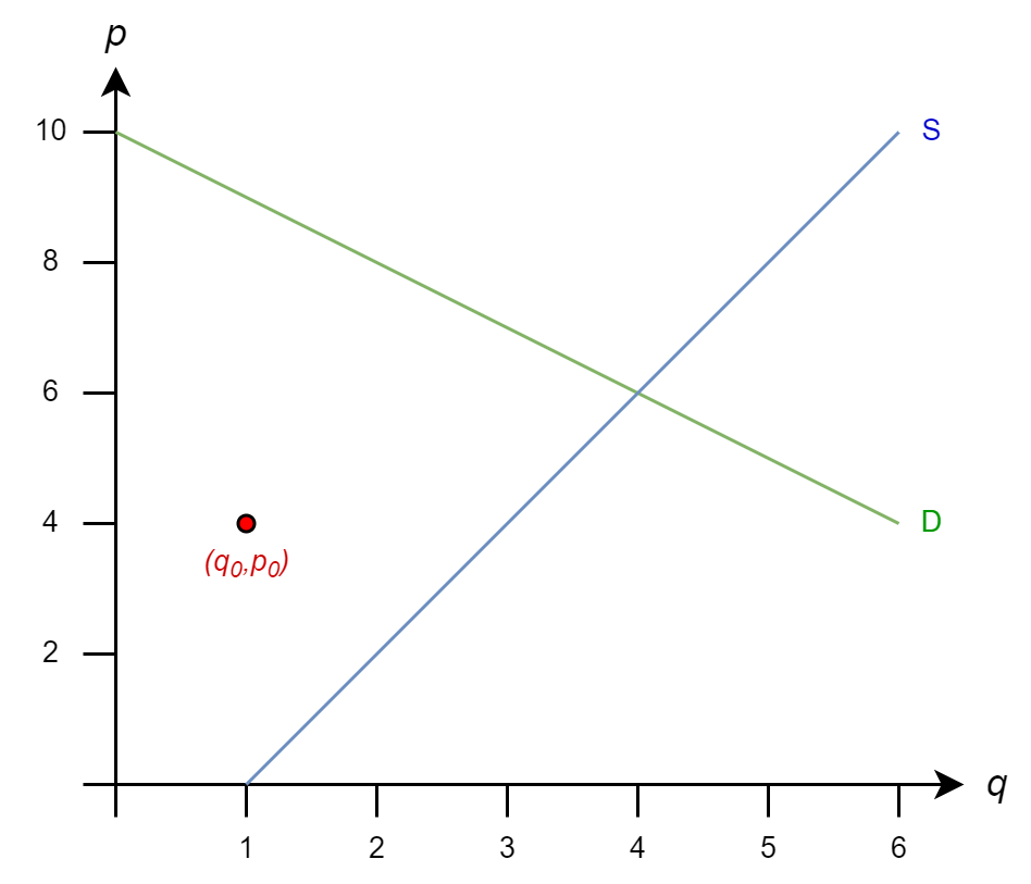
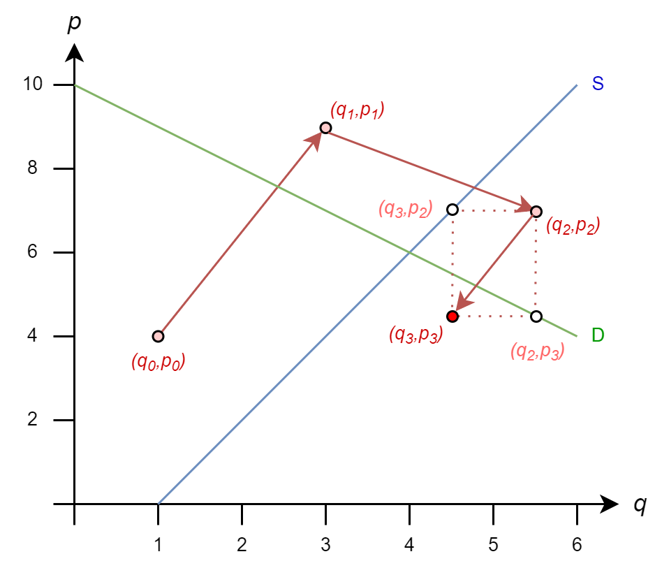
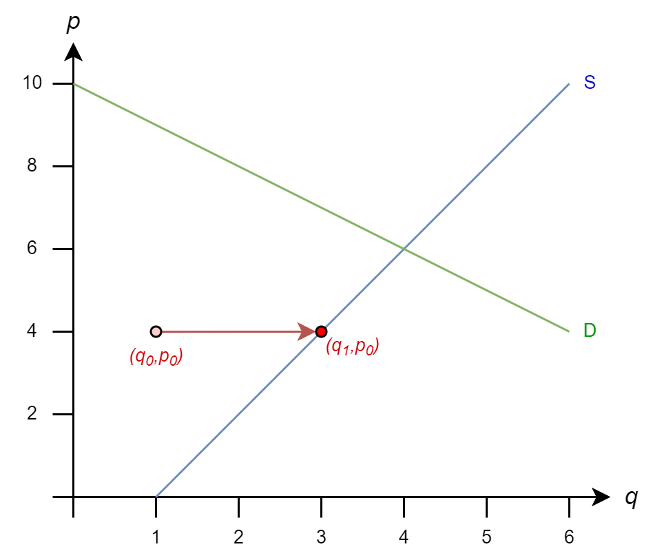
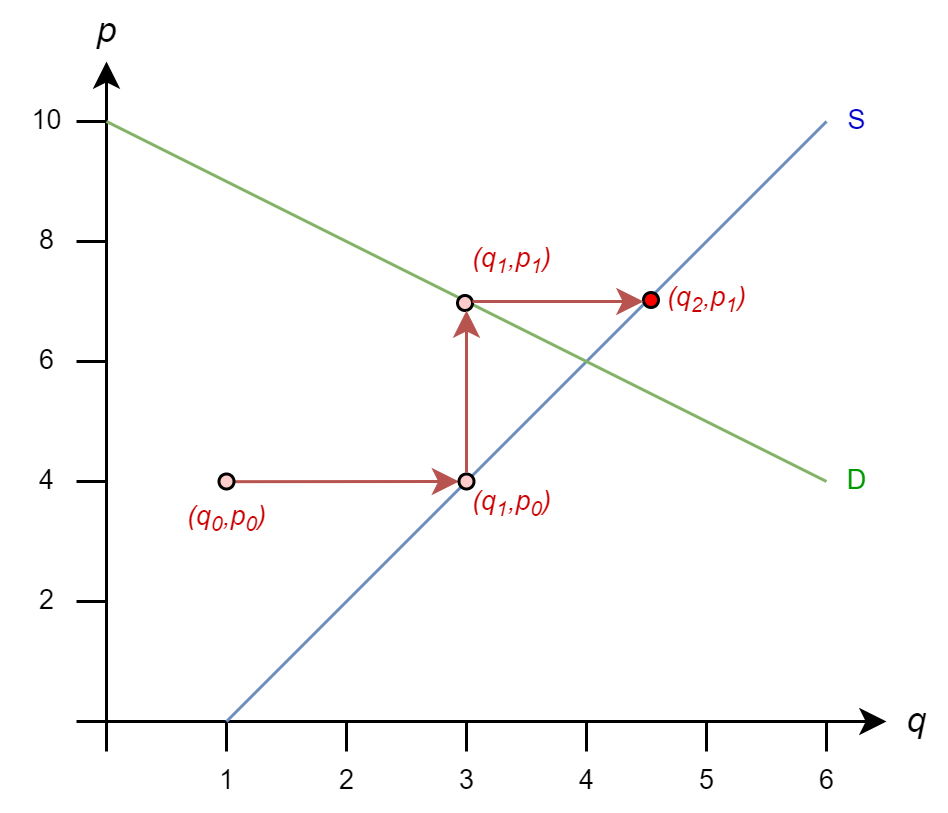
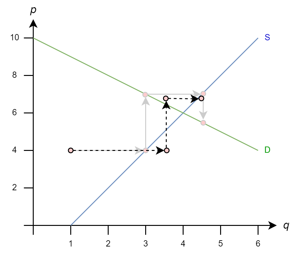
Let’s start from initial guess \(q_0=1\) and \(p_0=4\) and see how Gauss-Jacobi proceeds
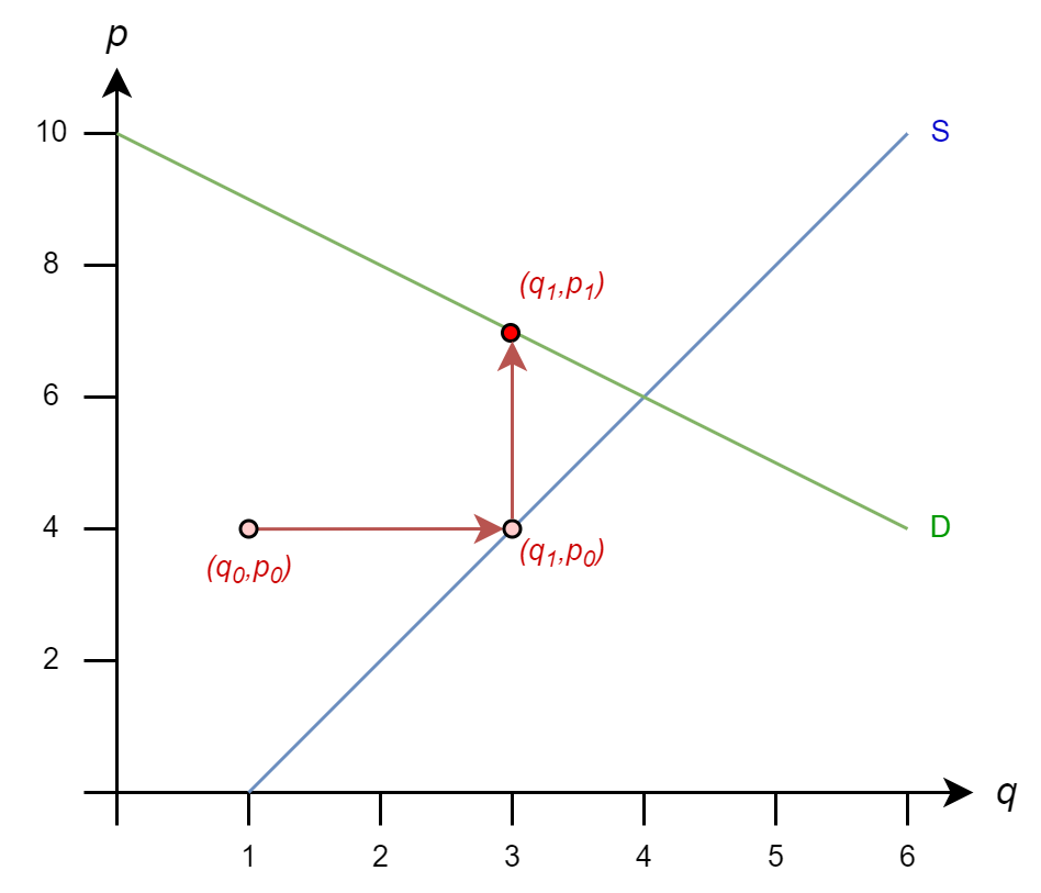
The iteration rules are
\(q^{(k+1)} = 1 + p^{(k)}/2\)
\(p^{(k+1)} = 10 - q^{(k)}\)
The iteration rules are
\(q^{(k+1)} = 1 + p^{(k)}/2\)
\(p^{(k+1)} = 10 - q^{(k)}\)
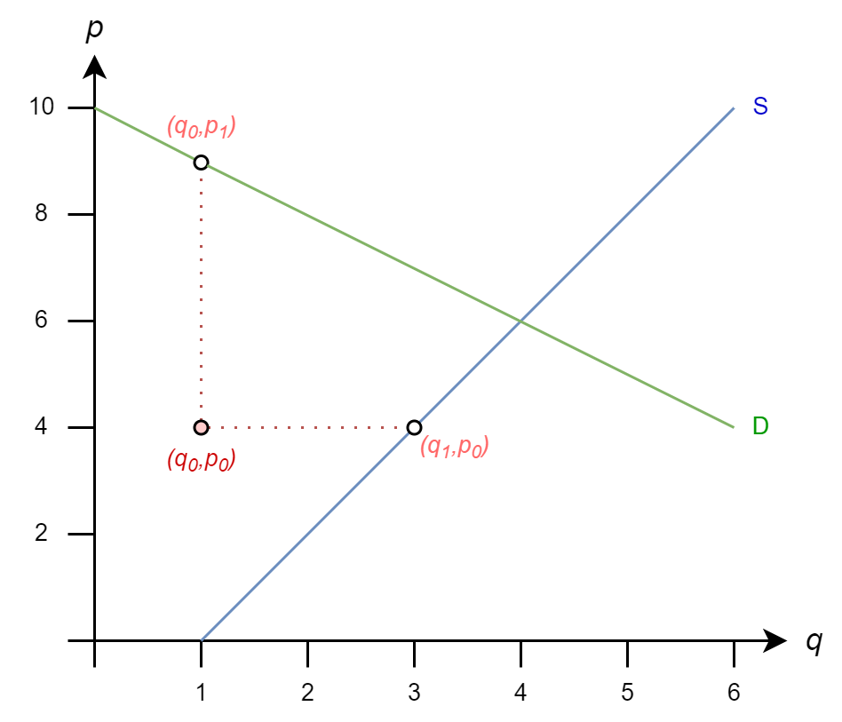
So
\(q_1 = 1 + (4)/2 = 3\)
The iteration rules are
\(q^{(k+1)} = 1 + p^{(k)}/2\)
\(p^{(k+1)} = 10 - q^{(k)}\)
So
\(q_1 = 1 + (4)/2 = 3\)
\(p_1 = 10 - 1 = 9\)
The iteration rules are
\(q^{(k+1)} = 1 + p^{(k)}/2\)
\(p^{(k+1)} = 10 - q^{(k)}\)
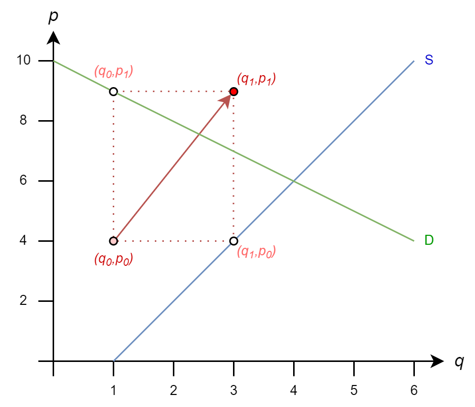
So
\(q_1 = 1 + (4)/2 = 3\)
\(p_1 = 10 - 1 = 9\)
And we move to \((3,9)\)
The iteration rules are
\(q^{(k+1)} = 1 + p^{(k)}/2\)
\(p^{(k+1)} = 10 - q^{(k)}\)
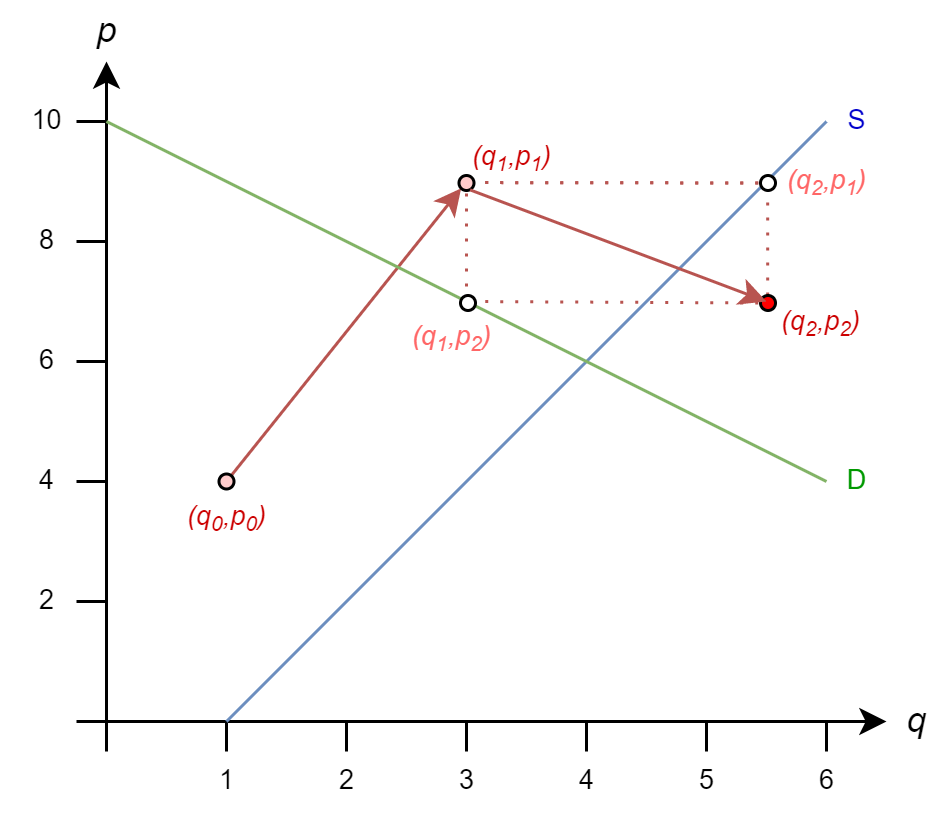
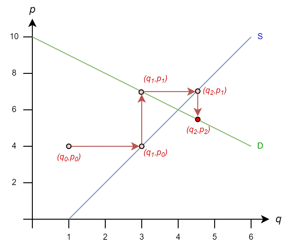
Next, we get
\(q_2 = 1 + (9)/2 = 5.5\)
\(p_2 = 10 - 3 = 7\)
And we move to \((5.5,7)\)
The iteration rules are
\(q^{(k+1)} = 1 + p^{(k)}/2\)
\(p^{(k+1)} = 10 - q^{(k)}\)
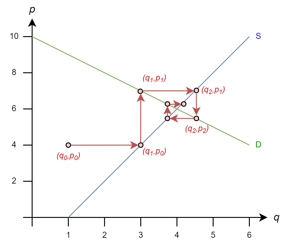
Then, we get
\(q_3 = 1 + (7)/2 = 4.5\)
\(p_3 = 10 - 5.5 = 4.5\)
And we move to \((4.5,4.5)\)
The iteration rules are
\(q^{(k+1)} = 1 + p^{(k)}/2\)
\(p^{(k+1)} = 10 - q^{(k)}\)
And we continue to process until the difference between \((q^{(k+1)},p^{(k+1)})\) and \((q^{(k)},p^{(k)})\) is smaller than our tolerance parameter (i.e., it converges)
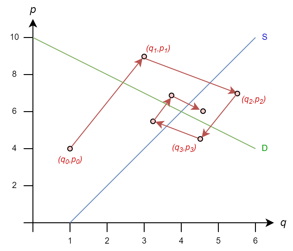
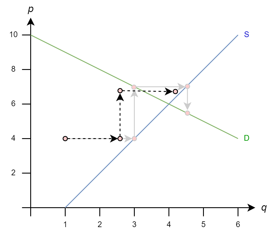
The Gauss-Seidel iteration rules looks similar, but there is an important difference
\[ \begin{align*} q^{(k+1)} & = 1 + p^{(k)}/2 \\ p^{(k+1)} & = 10 - \mathbf{q^{(k+1)}} \end{align*} \]
\(p^{(k+1)}\) is a function of \(q^{(k+1)}\), not \(q^{(k)}\)
Let’s see how that rule comes from matrix form
\[ A= \begin{bmatrix} 1 & 1 \\ 1 & -2 \\ \end{bmatrix} \Rightarrow Q = \begin{bmatrix} 1 & 1 \\ 0 & -2 \\ \end{bmatrix} \Rightarrow Q^{-1} = \begin{bmatrix} 1 & 1/2 \\ 0 & -1/2 \\ \end{bmatrix} \]
So \(x^{(k+1)} = Q^{-1}b + (I - Q^{-1}A)x^{(k)}\) gives
\[ \begin{bmatrix} p^{(k+1)} \\ q^{(k+1)} \\ \end{bmatrix} = \begin{bmatrix} 1 & 1/2 \\ 0 & -1/2 \\ \end{bmatrix} \begin{bmatrix} 10 \\ -2 \end{bmatrix} +\left( \begin{bmatrix} 1 & 0 \\ 0 & 1 \\ \end{bmatrix} - \begin{bmatrix} 1 & 1/2 \\ 0 & -1/2 \\ \end{bmatrix} \begin{bmatrix} 1 & 1 \\ 1 & -2 \\ \end{bmatrix} \right) \begin{bmatrix} p^{(k)} \\ q^{(k)} \\ \end{bmatrix} \]
\[ \begin{bmatrix} p^{(k+1)} \\ q^{(k+1)} \\ \end{bmatrix} = \begin{bmatrix} 9 \\ 1 \end{bmatrix} + \begin{bmatrix} -1/2 & 0 \\ 1/2 & 0 \\ \end{bmatrix} \begin{bmatrix} p^{(k)} \\ q^{(k)} \\ \end{bmatrix} \]
Once again, we start from initial guess \(q_0=1\) and \(p_0=4\)
The iteration rules are
\(q^{(k+1)} = 1 + p^{(k)}/2\)
\(p^{(k+1)} = 10 - q^{(k+1)}\)
The iteration rules are
\(q^{(k+1)} = 1 + p^{(k)}/2\)
\(p^{(k+1)} = 10 - q^{(k+1)}\)
So
\(q_1 = 1 + (4)/2 = 3\)
The iteration rules are
\(q^{(k+1)} = 1 + p^{(k)}/2\)
\(p^{(k+1)} = 10 - q^{(k+1)}\)
So
\(q_1 = 1 + (4)/2 = 3\)
\(p_1 = 10 - (3) = 7\)
The iteration rules are
\(q^{(k+1)} = 1 + p^{(k)}/2\)
\(p^{(k+1)} = 10 - q^{(k+1)}\)
So
\(q_1 = 1 + (4)/2 = 3\)
\(p_1 = 10 - (3) = 7\)
\(q_2 = 1 + (7)/2 = 4.5\)
The iteration rules are
\(q^{(k+1)} = 1 + p^{(k)}/2\)
\(p^{(k+1)} = 10 - q^{(k+1)}\)
So
\(q_1 = 1 + (4)/2 = 3\)
\(p_1 = 10 - (3) = 7\)
\(q_2 = 1 + (7)/2 = 4.5\)
\(p_2 = 10 - 4.5 = 5.5\)
The iteration rules are
\(q^{(k+1)} = 1 + p^{(k)}/2\)
\(p^{(k+1)} = 10 - q^{(k+1)}\)
And we continue to process until the difference between \((q^{(k+1)},p^{(k+1)})\) and \((q^{(k)},p^{(k)})\) is smaller than our tolerance parameter (i.e., it converges)
These methods are conceptually simple: we will multiply our step \(x^{(k)}\rightarrow x^{(k+1)}\) by a scalar \(\omega\)
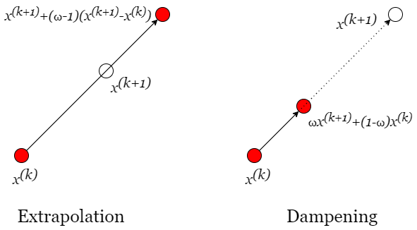
Returning to our Gauss-Seidel example, accelerating the solution with extrapolation could look like this
And, stabilizing the solution with dampening could look like this
These methods don’t always work. It may be a good idea to try if you are having issues with slow convergence or divergence
We’ll skip the technical details of when these methods work for operator splitting