x_i is some evaluation point (e.g. midpoint of dx_i)
1.3 Infinite limits strike again
Just like derivatives, we face an infinite limit because as {dx_i} \rightarrow 0, \frac{(a-b)}{dx_i} \rightarrow \infty
. . .
We avoid this issue in the same way as derivatives: we replace the infinite sum with something we can handle
. . .
We will see two types of methods:
Stochastic approximation with Monte Carlo
Quadrature
2 Monte Carlo integration
2.1 Monte Carlo integration
It’s probably the most commonly used form in empirical economics
. . .
Key idea: approximate an integral by relying on LLN and “randomly”sampling the integration domain
. . .
Can be effective for very-high-dimensional integrals
Very simple and intuitive
But produces a random approximation
2.2 Monte Carlo integration
We integrate
\xi = \int_0^1 f(x) dx
by drawing N uniform samples, x_1,\dots,x_N over interval [0,1]
. . .
\xi is equivalent to E[f(x)] with respect to a uniform distribution, so estimating the integral is the same as estimating the expected value of f(x)
. . .
In general we have that \hat{\xi} = V\frac{1}{N}\sum_{i=1}^N f(x_i), where V is the volume over which we are integrating
. . .
LLN gives us that the plim_{N\rightarrow\infty} \hat{\xi} = \xi
2.3 Monte Carlo integration
The variance of \hat{\xi} is \sigma^2_{\hat{\xi}} = Var(\frac{V}{N}\sum_{i=1}^N f(x_i)) = \frac{V^2}{N^2} \sum_{i=1}^N Var(f(X)) = \frac{V^2}{N}\sigma^2_{f(X)}
. . .
So average error is \frac{V}{\sqrt{N}}\sigma_{f(X)}. This gives us its rate of convergence: O(1/\sqrt{N})
Notes:
The rate of convergence is independent of the dimension of x
Quasi-Monte Carlo methods can get you O(1/N)
These methods have a smarter approach to sampling
They use nonrandom sequences like so they cover the support in more efficient ways (see details on Ch 5.4 of Miranda and Fackler)
2.4 Monte Carlo integration
Suppose we want to integrate x^2 from 0 to 10, we know this is 10^3/3 = 333.333
Code
# Package for drawing random numbersusingDistributions# Define a function to do the integration for an arbitrary functionfunctionintegrate_mc(f, lower, upper, num_draws)# Draw from a uniform distribution xs =rand(Uniform(lower, upper), num_draws)# Expectation = mean(x)*volume expectation =mean(f(xs))*(upper - lower)end
integrate_mc (generic function with 1 method)
2.5 Monte Carlo integration
Suppose we want to integrate x^2 from 0 to 10, we know this is 10^3/3 = 333.333
Code
f(x) = x.^2;integrate_mc(f, 0, 10, 1000)
320.7085212559472
Quite close for a random process!
3 Quadrature: Newton-Cotes
3.1 Quadrature integration types
We can also approximate integrals using a technique called quadrature
. . .
With quadrature we effectively take weighted sums to approximate integrals
. . .
We will focus on two classes of quadrature for now:
Newton-Cotes (the kind you’ve seen before)
Gaussian (probably new)
3.2 Newton-Cotes quadrature rules
Suppose we want to integrate a one dimensional function f(x) over [a,b]
How would you do it?
. . .
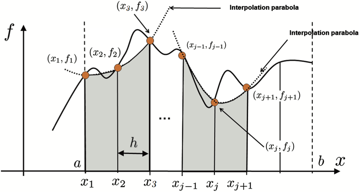
One answer is to replace the function with something easier to integrate: a piece-wise polynomial
. . .
Key things to define up front:
x_i = a + (i-1)/h for i=1,2,...,n where h = \frac{b-a}{n-1}
x_is are the quadrature nodes of the approximation scheme and divide the interval into n-1 evenly spaced subintervals of length h
3.3 Midpoint rule
Most basic Newton-Cotes method:
Split [a,b] into intervals
Approximate the function in each subinterval by a constant equal to the function at the midpoint of the subinterval
Let’s integrate x^2 again from 0 to 100 (the answer is 333.33…)
Code
# Generic function to integrate with midpointfunctionintegrate_midpoint(f, a, b, N)# Calculate h given the interval [a,b] and N nodes h = (b-a)/(N-1)# Calculate the nodes starting from a+h/2 til b-h/2 x =collect(a+h/2:h:b-h/2)# Calculate the expectation expectation =sum(h*f(x))end;
3.6 Midpoint rule: let’s code it up
Code
f(x) = x.^2;println("Integrating with 5 nodes:$(integrate_midpoint(f, 0, 10, 5))")println("Integrating with 50 nodes:$(integrate_midpoint(f, 0, 10, 50))")println("Integrating with 100 nodes:$(integrate_midpoint(f, 0, 10, 100))")
Integrating with 5 nodes:328.125
Integrating with 50 nodes:333.29862557267813
Integrating with 100 nodes:333.3248307995783
. . .
Decent approximation with only 5 nodes. We get pretty close to the answer once we move up to 100 nodes.
3.7 Trapezoid rule
Increase complexity by 1 degree:
Split [a,b] into intervals
Approximate the function in each subinterval by a linear interpolation passing through (x_i,f(x_i)) and (x_{i+1},f(x_{i+1}))
where w_1=w_n = h/3, otherwise and w_i = 4h/3 if i is even and w_i = 2h/3 if i is odd
3.12 Simpson’s rule
3.13 How accurate is this rule?
Simpson’s rule is O(h^4) and third-order exact: it can integrate any cubic function exactly
. . .
That’s weird! Why do we gain 2 orders of accuracy when increasing one order of approximation complexity?
. . .
The approximating piecewise quadratic is exact at the end points and midpoint of the conjoined two subintervals
. . .
The difference between a cubic f(x) and the quadratic approximation in [x_{2i-1},x_{2i+1}] is another cubic function
. . .
This cubic function is odd with respect to the midpoint \rightarrow integrating over the first subinterval cancels integrating over the second subinterval
3.14 Note on accuracy
The derivation of the order of error terms is similar to what we did for forward differences: we use Taylor expansions
But there are some extra steps because we have to bring the integral in. We’re going to skip these derivations
BUT it is important to know that these derivations assume smooth functions. That might not be the case in economic models because corner solutions might exist!
Simpson’s is more accurate than the trapezoid rule for smooth functions
But for functions with kinks/discontinuities in the 1st derivative, the trapezoid rule is often more accurate than Simpson’s
3.15 Higher order integration
We can generalize the unidimensional Newton-Cotes quadrature with tensor products
We compute separately the n_1 nodes and weights (x_{1i}, w_{1i}) and n_2 for (x_{2j}, w_{2j}). The tensor product will give us a grid with n = n_1 n_2 points
Gaussian rules are 2n-1 order exact: we can exactly compute the integral of any polynomial order 2n-1
4.4 Gaussian quadrature takeaways
Gaussian quadrature effectively discretizes some distribution p(x) into mass points (nodes) and probabilities (weights) for some other discrete distribution \bar{p}(x)
. . .
Given an approximation with n mass points, X and \bar{X} have identical moments up to order 2n
As n\rightarrow\infty we have a continuum of mass points and recover the continuous pdf
. . .
But what do we pick for the weighting function w(s)?
4.5 Gauss-Legendre
We can start out with a simple w(s) = 1: this gives us Gauss-Legendre quadrature
This can approximate the integral of any function arbitrarily well by increasing n
4.6 Gauss-Laguerre
Sometimes we want to compute exponentially discounted sums like
\int_I f(s) e^{-s} ds
The weighting function e^{-s} is Gauss-Laguerre quadrature
. . .
In economics, this method is particularly suited for applications with continuous-time discounting
4.7 Gauss-Hermite
Sometimes we want to take expectations of functions of normally distributed variables
\int_I f(s) e^{-s^2} ds
. . .
Other methods exist for specialized functional forms/distributions: gamma, beta, chi-square, etc
4.8 Gaussian quadrature nodes and weights
OK, Gaussian quadrature sounds nice. But how do we actually find the nodes and weights?
. . .
It’s a non-trivial task: we have to solve 2n nonlinear equations to get n pairs (x_i, w_n)
We’ll use a package for that: QuantEcon.jl
(QuantEcon functions are also implemented in Python: QuantEconPy)
Another package FastGaussQuadrature.jl does a better job with high-order integrals or weights with singularities
QuadGK has methods to improve precision further with adaptive subdomains
4.9QuantEcon.jl: Gaussian quadrature
Let’s go back to our previous example and integrate x^2 from 0 to 10 again (the answer is 333.333…)
Code
usingQuantEcon;# Our generic function to integrate with Gaussian quadraturefunctionintegrate_gauss(f, a, b, N)# This function get nodes and weights for Gauss-Legendre quadrature x, w =qnwlege(N, a, b)# Calculate expectation expectation =sum(w .*f(x))end;
4.10QuantEcon.jl: Gaussian quadrature
Code
f(x) = x.^2;println("Integrating with 1 node:$(integrate_gauss(f, 0, 10, 1))")println("Integrating with 2 nodes:$(integrate_gauss(f, 0, 10, 2))")
Integrating with 1 node:250.0
Integrating with 2 nodes:333.3333333333334
. . .
All we needed was 2 nodes!
We need 1000 draws with Monte Carlo and 100 nodes with midpoint to get limited approximations
Gauss-Hermite (qnwnorm) or Gaussian with any continuous distribution (qnwdist)
Generic quadrature integration (quadrect)
4.12 Practice integration with QuantEcon.jl
Let’s integrate f(x) = \frac{1}{x^2 + 1} from 0 to 1
Tip: Type ? in the REPL and the name of the function to read its documentation and learn how to call it
Use quadrect to integrate using Monte Carlo
You will need to code your function f to accept an array (. syntax)
Use qnwtrap to integrate using the Trapezoid rule quadrature
Use qnwlege to integrate using Gaussian quadrature
. . .
Do we know what is the analytic solution to this integral?
4.13 Practice integration with QuantEcon.jl
Show the code
f(x) =1.0./(x.^2.+1.0);# 1. Use `quadrect` to integrate using Monte Carlo with 1000 nodesquadrect(f, 1000, 0.0, 1.0, "R")
0.7896227636186307
Show the code
# 2. Use `qnwtrap` to integrate using the Trapezoid rule quadrature with 7 nodesx, w =qnwtrap(7, 0.0, 1.0);# Perform quadrature approximationsum(w .*f(x))
0.7842407666178157
Show the code
# 3. Use `qnwlege` to integrate using Gaussian quadrature with 7 nodesx, w =qnwlege(7, 0.0, 1.0);# Perform quadrature approximationsum(w .*f(x))
0.785398164063432
. . .
By the way, \int^1_0 1/(x^2 + 1) = \arctan(1) = \pi/4
Code
π/4
0.7853981633974483
5 Applied example: Expected utility under quality uncertainty
5.1 Extra: Applied example
Computing expected utility under quality uncertainty
We’ll compare Trapezoid, Gauss-Legendre, and Gauss-Hermite quadrature on a problem that arises naturally in economics: taking expectations over normally distributed shocks
5.2 Setup: Cobb-Douglas with uncertain quality
A consumer has Cobb-Douglas utility over two goods x_1, x_2 with an uncertain quality shifter \theta on good 2:
where z = \ln\theta. Can you compute this integral by hand?
5.3 Why this problem is a good test case
This integral has a known closed-form solution. Since e^{(1-\alpha)z} with z \sim N(\mu, \sigma^2) is exactly the MGF of the normal evaluated at 1-\alpha, we have:
So we can check exactly how well each numerical method does
5.4 Tangent: How did we get the closed-form solution?
The integral we need is E[e^{(1-\alpha)z}] where z = \ln\theta \sim N(\mu, \sigma^2). This happens to be the moment generating function of the normal evaluated at t = (1-\alpha)
. . .
The MGF of z \sim N(\mu, \sigma^2) is M_z(t) = E[e^{tz}] = \exp\left(t\mu + \frac{t^2 \sigma^2}{2}\right)
. . .
Derivation: the product e^{tz} \cdot \phi(z) has combined exponent
Let’s set \alpha = 0.4, x_1 = 2, x_2 = 3, \mu = 0, \sigma = 0.5 and calculate the true value
Code
usingQuantEcon, Plots, Distributions, LaTeXStrings;# Parametersα =0.4x₁, x₂ =2.0, 3.0μ, σ =0.0, 0.5# The integrand: g(z) * ϕ(z) where g(z) = x₁^α * (exp(z)*x₂)^(1-α) and ϕ is Normal pdfg(z) = x₁^α * (exp.(z) .* x₂).^(1-α)# Analytic solution via MGF of normal distributionEU_true = x₁^α * x₂^(1-α) *exp((1-α)*μ +0.5*(1-α)^2*σ^2)println("True expected utility: $(round(EU_true, digits=8))")
True expected utility: 2.66825912
5.7 Method 1: Trapezoid rule
The trapezoid rule needs a finite interval, so we truncate the normal at \mu \pm 4\sigma and integrate g(z)\phi(z) directly
Code
functioneu_trapezoid(n) a, b = μ -4σ, μ +4σ # Truncated domain x, w =qnwtrap(n, a, b)# We must include the normal pdf in the integrand ϕ =pdf.(Normal(μ, σ), x)returnsum(w .*g(x) .* ϕ)end;for n in [5, 11, 21, 51] eu =eu_trapezoid(n) err =abs(eu - EU_true)println("Trapezoid n=$n: EU=$(round(eu, digits=8)), error=$(round(err, sigdigits=3))")end
Same truncation strategy, but now nodes are not evenly spaced: they cluster where they matter most for polynomial exactness
Code
functioneu_legendre(n) a, b = μ -4σ, μ +4σ x, w =qnwlege(n, a, b) ϕ =pdf.(Normal(μ, σ), x)returnsum(w .*g(x) .* ϕ)end;for n in [5, 11, 21, 51] eu =eu_legendre(n) err =abs(eu - EU_true)println("Legendre n=$n: EU=$(round(eu, digits=8)), error=$(round(err, sigdigits=3))")end
Notice Gauss-Hermite needs far fewer nodes. The weight function e^{-x^2} is doing the heavy lifting
5.10 Convergence comparison
Show the code
ns_trap =3:2:51# odd numbers for compatibilityns_lege =3:2:51ns_herm =3:2:11errs_trap = [abs(eu_trapezoid(n) - EU_true) for n in ns_trap]errs_lege = [abs(eu_legendre(n) - EU_true) for n in ns_lege]errs_herm = [abs(eu_hermite(n) - EU_true) for n in ns_herm]plot(ns_trap, errs_trap, label="Trapezoid", lw=2, marker=:circle, ms=3, yscale=:log10, xlabel="Number of nodes", ylabel="Absolute error (log scale)", title="Convergence: Expected utility of Cobb-Douglas", legend=:bottomright, size=(700, 400), ylims=(1e-16, 1e0))plot!(ns_lege, errs_lege, label="Gauss-Legendre", lw=2, marker=:square, ms=3)plot!(ns_herm, errs_herm, label="Gauss-Hermite", lw=2, marker=:diamond, ms=3)hline!([eps()], label="Machine epsilon", ls=:dash, color=:gray)
5.11 Why does Gauss-Hermite win here?
The integral has the form \int g(z) \phi(z) dz where \phi is the normal pdf
. . .
Trapezoid/Legendre: treat g(z)\phi(z) as a generic function and approximate it with evenly-spaced or Legendre-optimal nodes over a truncated interval
Gauss-Hermite: the weight function e^{-x^2}matches the kernel of the normal pdf, so the weights already account for the density. The nodes only need to approximate g(z), which is smooth and slowly varying
. . .
Takeaway: when your integrand has a known density component, choose the quadrature whose weight function matches it
5.12 Visualizing nodes and weights: n = 5
Let’s see where each method places its 5 nodes and how it weights them
Show the code
# Get nodes and weights for n=5x_t, w_t =qnwtrap(5, μ-4σ, μ+4σ)x_l, w_l =qnwlege(5, μ-4σ, μ+4σ)x_h, w_h =qnwnorm(5, μ, σ^2)# For Trapezoid and Legendre, effective weight = w * ϕ(x) (contribution to final sum)eff_t = w_t .*pdf.(Normal(μ, σ), x_t)eff_l = w_l .*pdf.(Normal(μ, σ), x_l)# For Hermite, the weights already incorporate the densityeff_h = w_hp1 =bar(x_t, eff_t, bar_width=0.03, label="Trapezoid", alpha=0.8, color=:steelblue, title="Effective weights (wᵢ × ϕ(xᵢ) or wᵢ for Hermite)", ylabel="Effective weight", xlabel=L"z = \ln\theta", legend=:topright, size=(700, 400))bar!(x_l, eff_l, bar_width=0.03, label="Gauss-Legendre", alpha=0.8, color=:coral)bar!(x_h, eff_h, bar_width=0.03, label="Gauss-Hermite", alpha=0.8, color=:seagreen)
Hermite concentrates nodes near the center of the distribution where the integrand has most mass. Trapezoid wastes nodes in the tails where \phi(z) \approx 0
5.14 Visualizing the Gauss-Hermite “discretization”
Remember: Gauss-Hermite discretizes the continuous normal into mass points
Show the code
# Compare the continuous normal pdf with the Hermite discrete approximation for n = 3, 5, 9ns_plot = [5, 9, 21]p_disc =plot(layout=(1,3), size=(800, 400), plot_title="Gauss-Hermite discretization of N($(μ), $(σ))")for (idx, n) inenumerate(ns_plot) xn, wn =qnwnorm(n, μ, σ^2)plot!(p_disc[idx], zz, pdf.(Normal(μ, σ), zz), lw=2, label="Normal pdf", color=:black)bar!(p_disc[idx], xn, wn ./0.05, bar_width=0.05, alpha=0.6, label="Hermite (n=$n)", color=:seagreen, xlabel=L"z", title="n = $n", legend=:topleft)# Scale: divide weights by bar width to get comparable density heightendp_disc
. . .
As n grows, the discrete distribution converges to the continuous one. This is the moment-matching at work