Nighttime Lights Analysis

Author

Data Lab

Published

September 20, 2024

Nighttime lights have become a commonly used resource to estimate changes in local economic activity. This document analyzes nighttime lights within the country.

Data

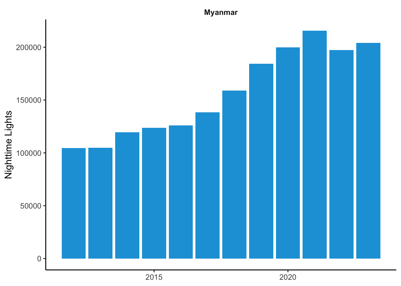
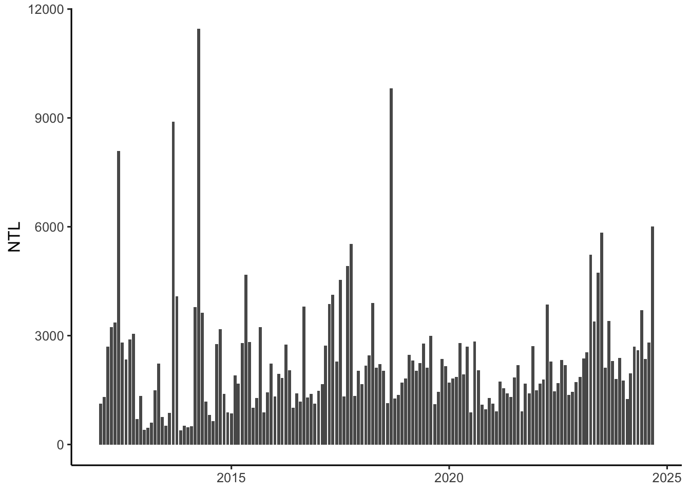
We use nighttime lights data from VIIRS Black Marble. Raw nighttime lights data requires correction due to cloud cover and stray light, such as lunar light. The Black Marble dataset applies advanced algorithms to correct raw nighttime light values and calibrate data so that trends in lights over time can be meaningfully analyzed. From VIIRS Black Marble, we use data from January 2012 through present—where data is available at a 500-meter resolution.

Methodology

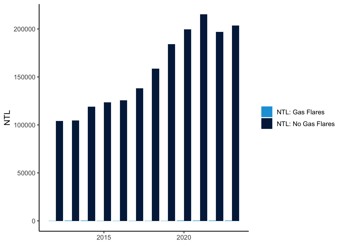
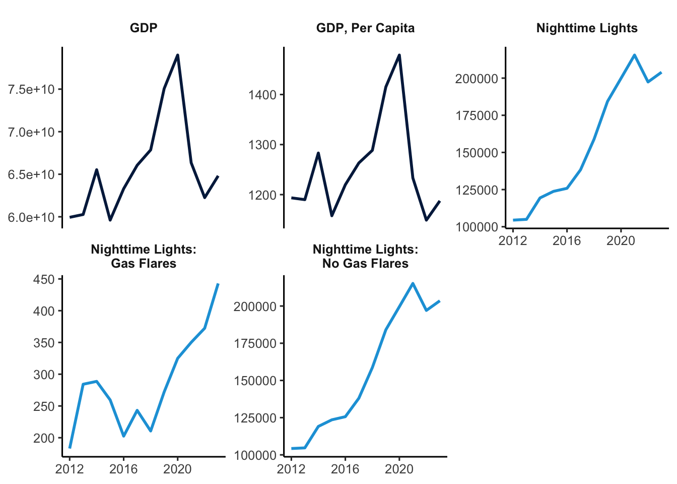
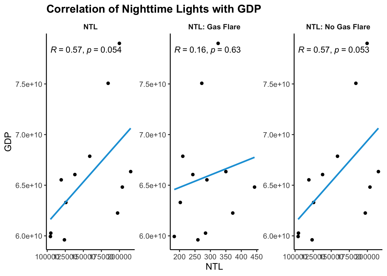
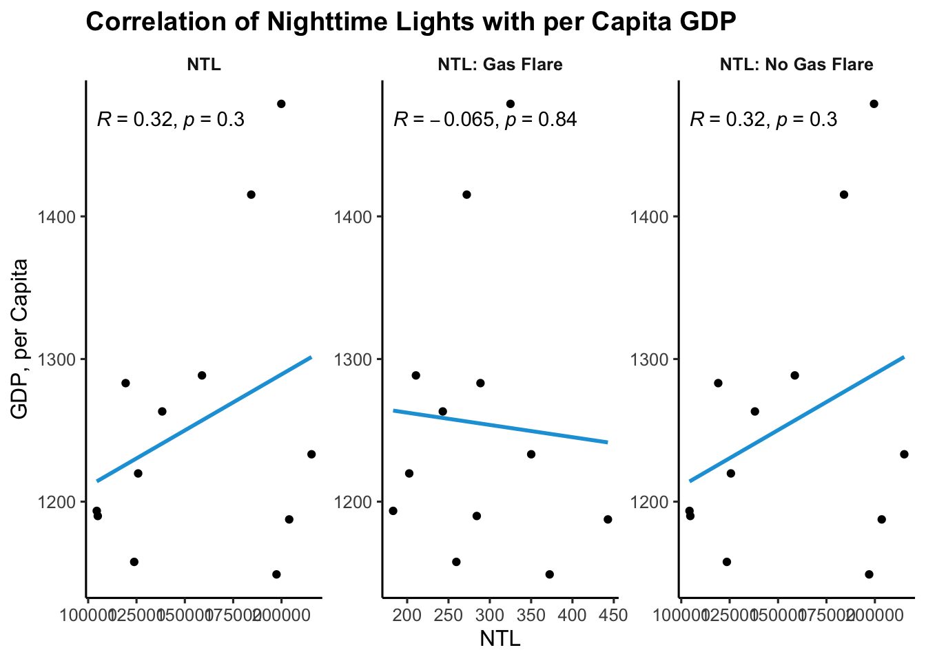
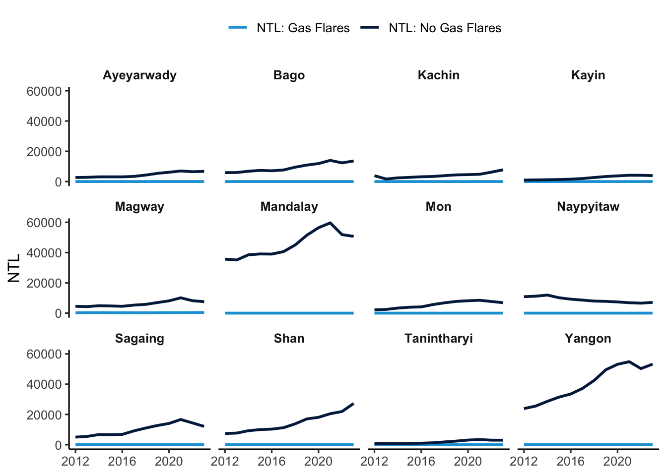
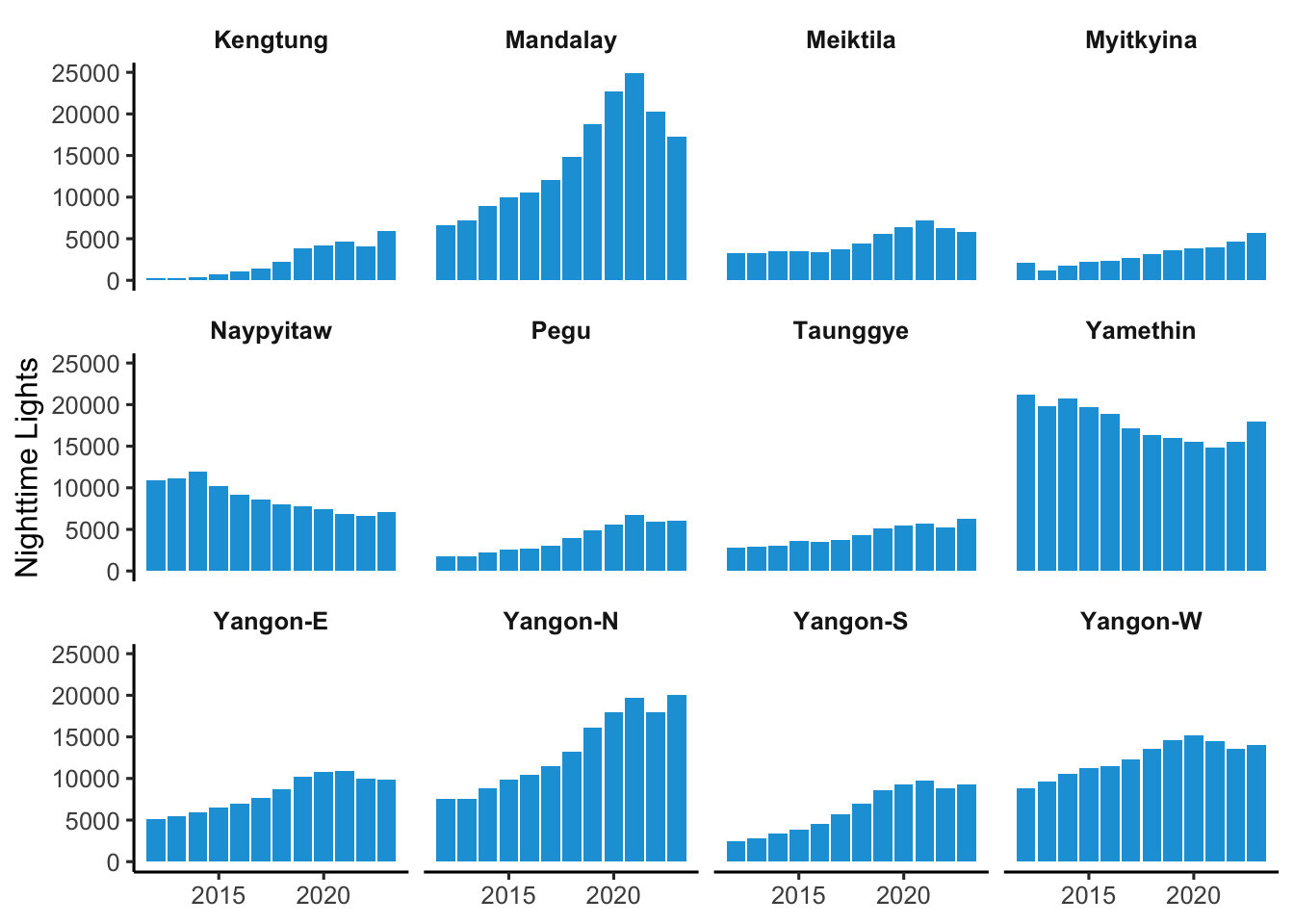
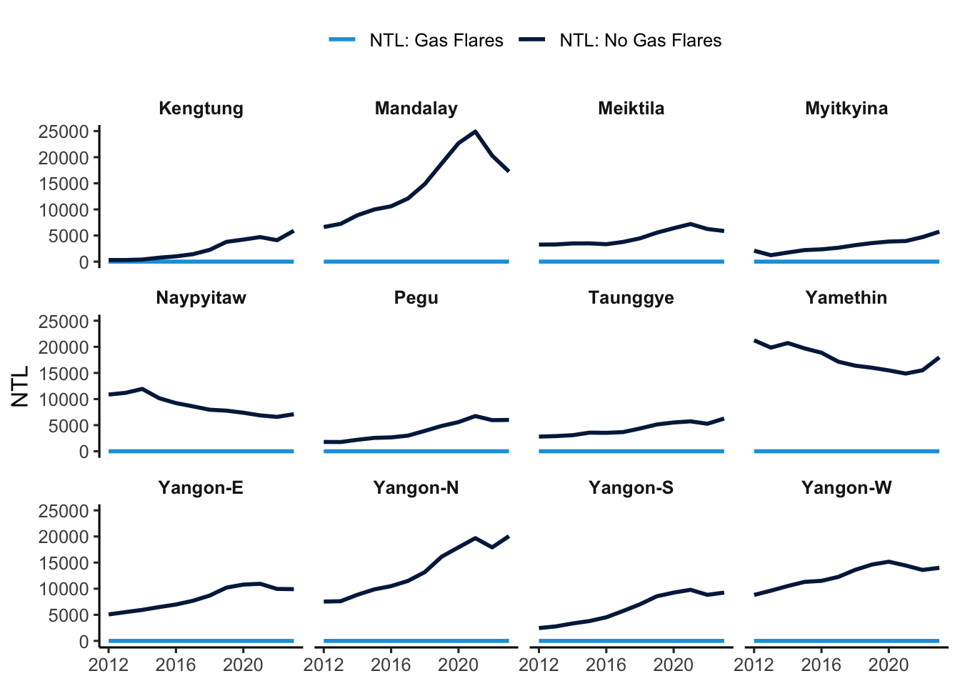
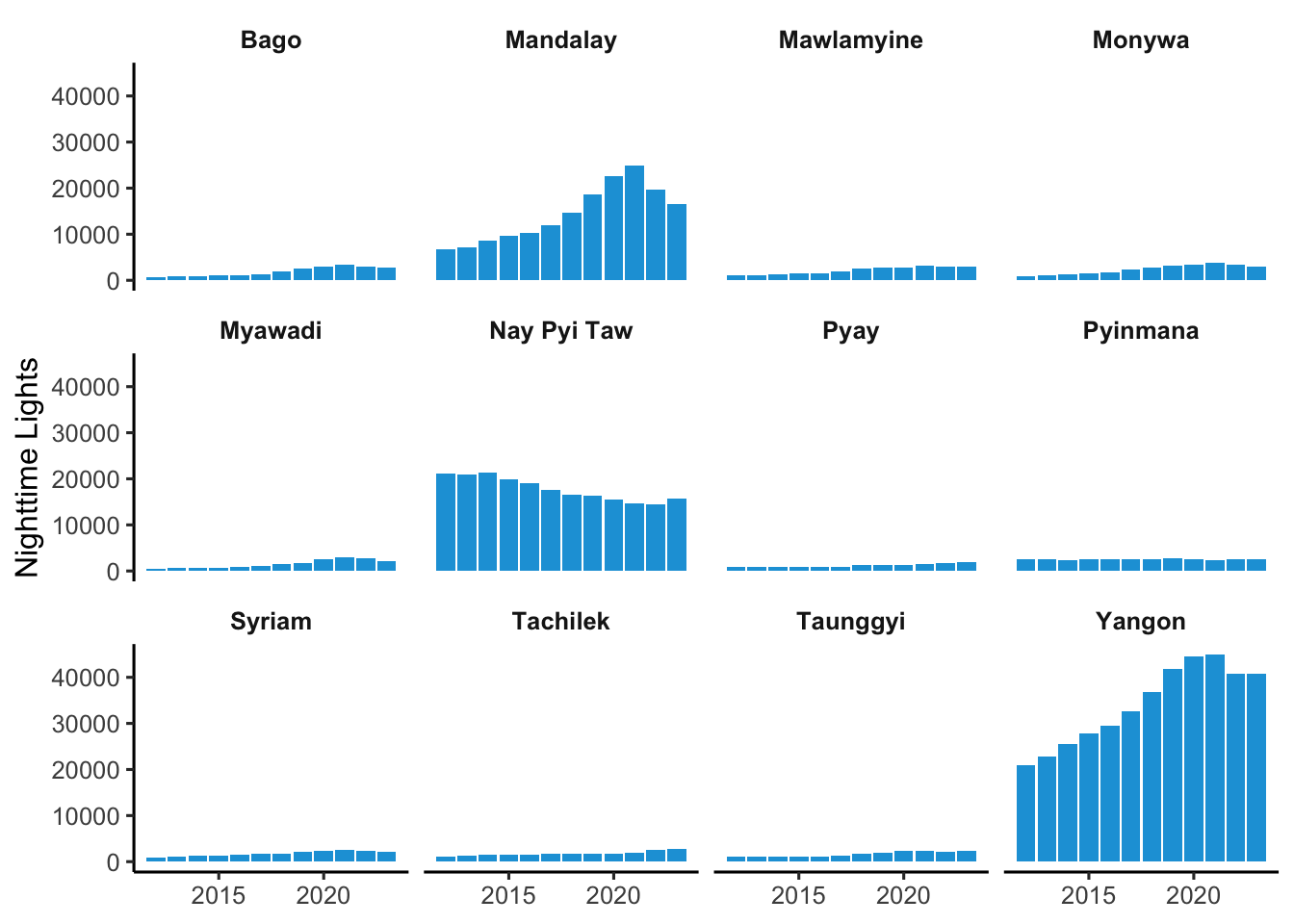
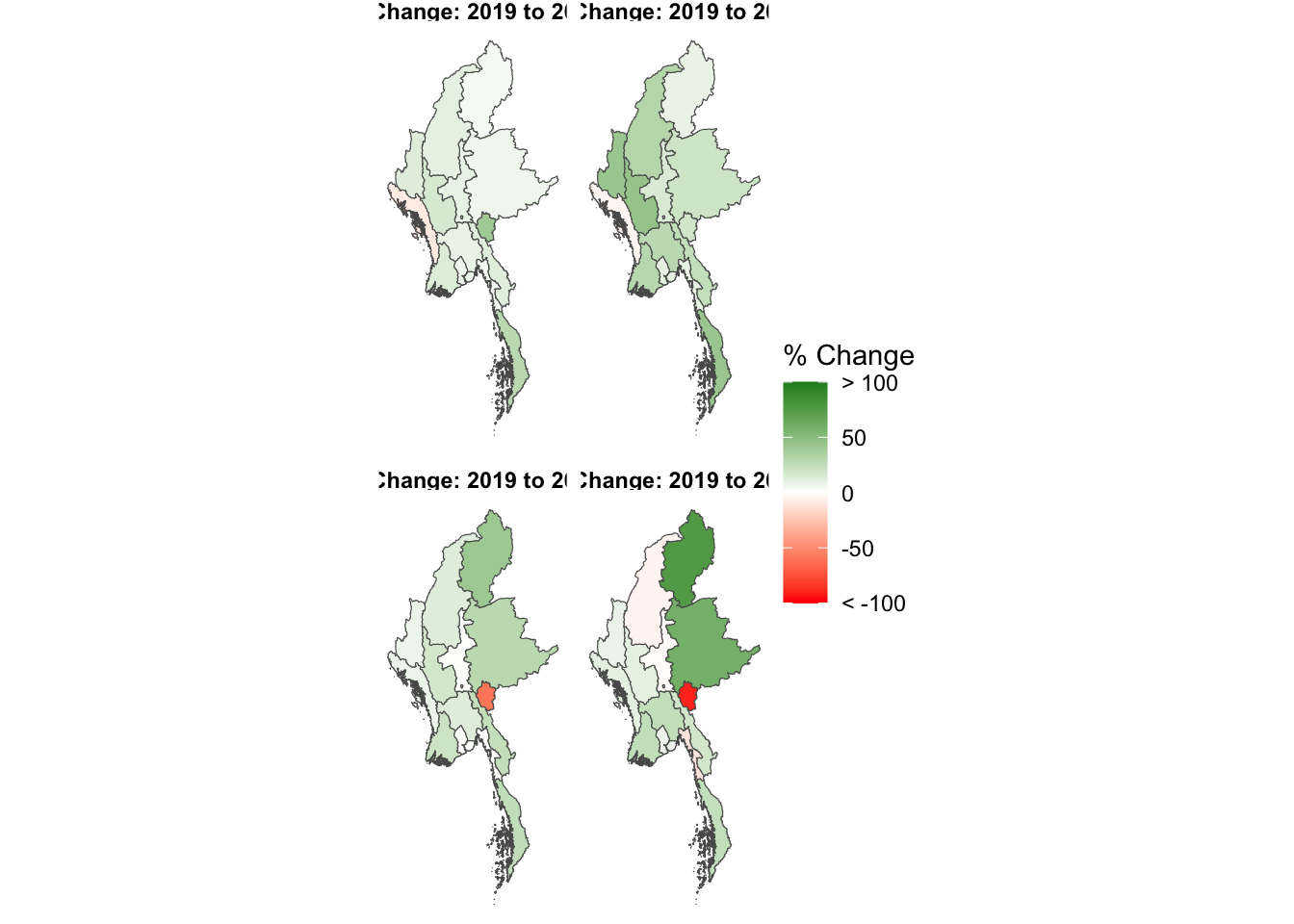
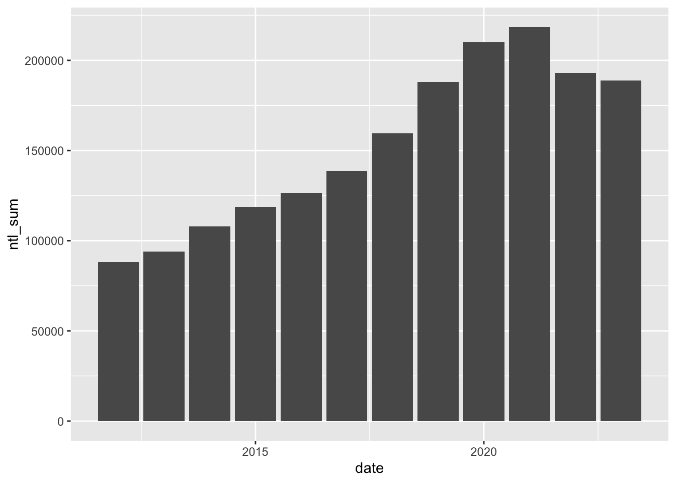
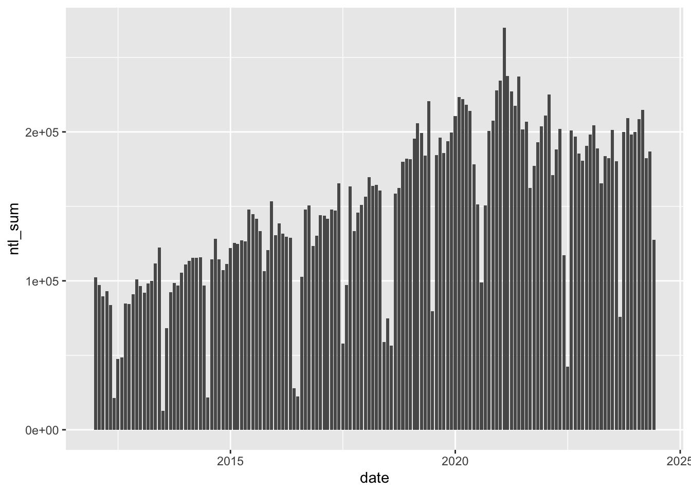
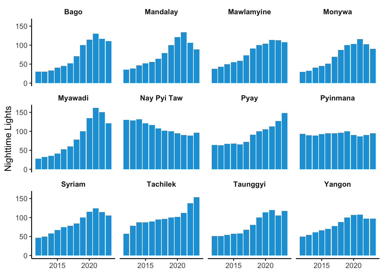
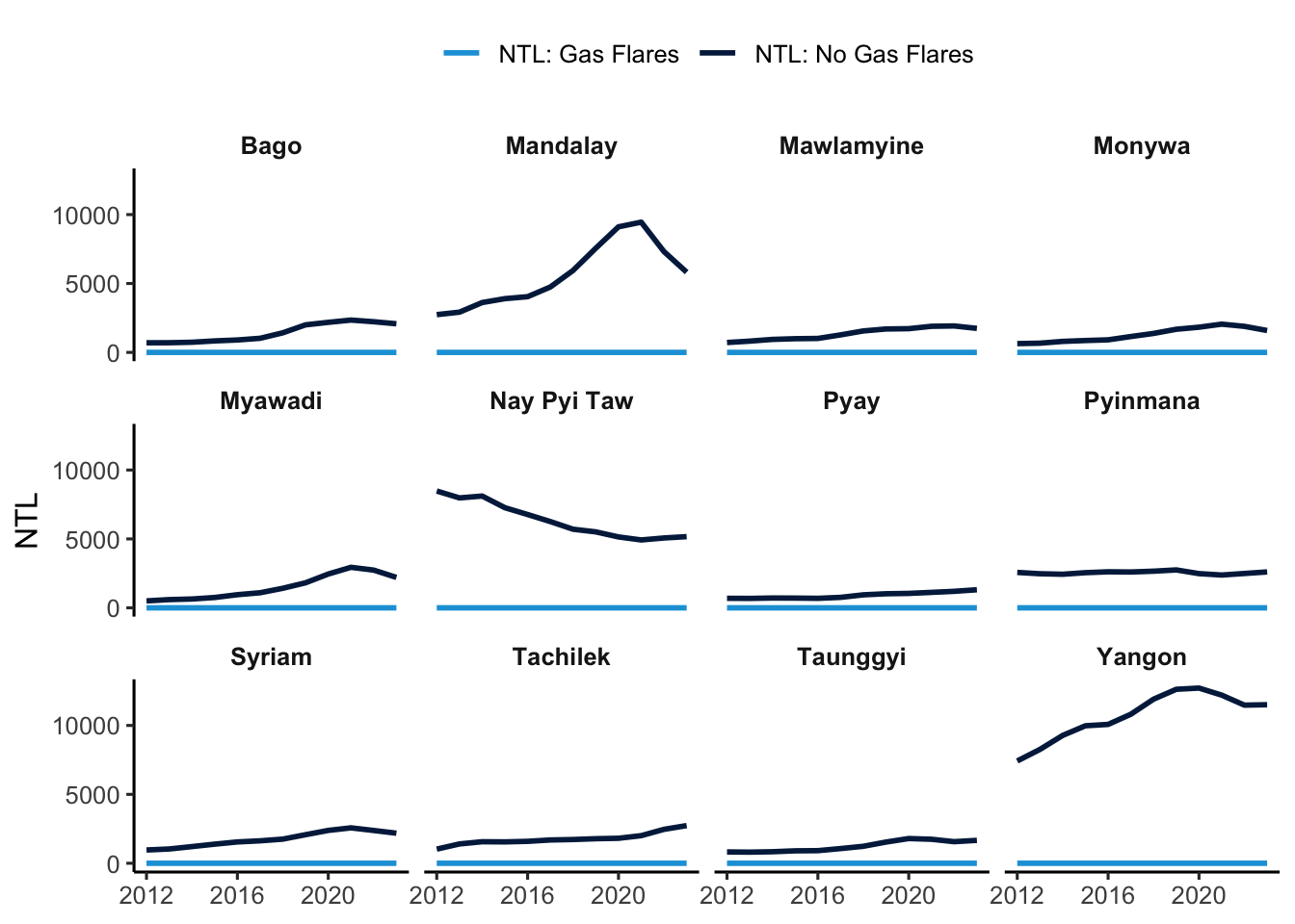
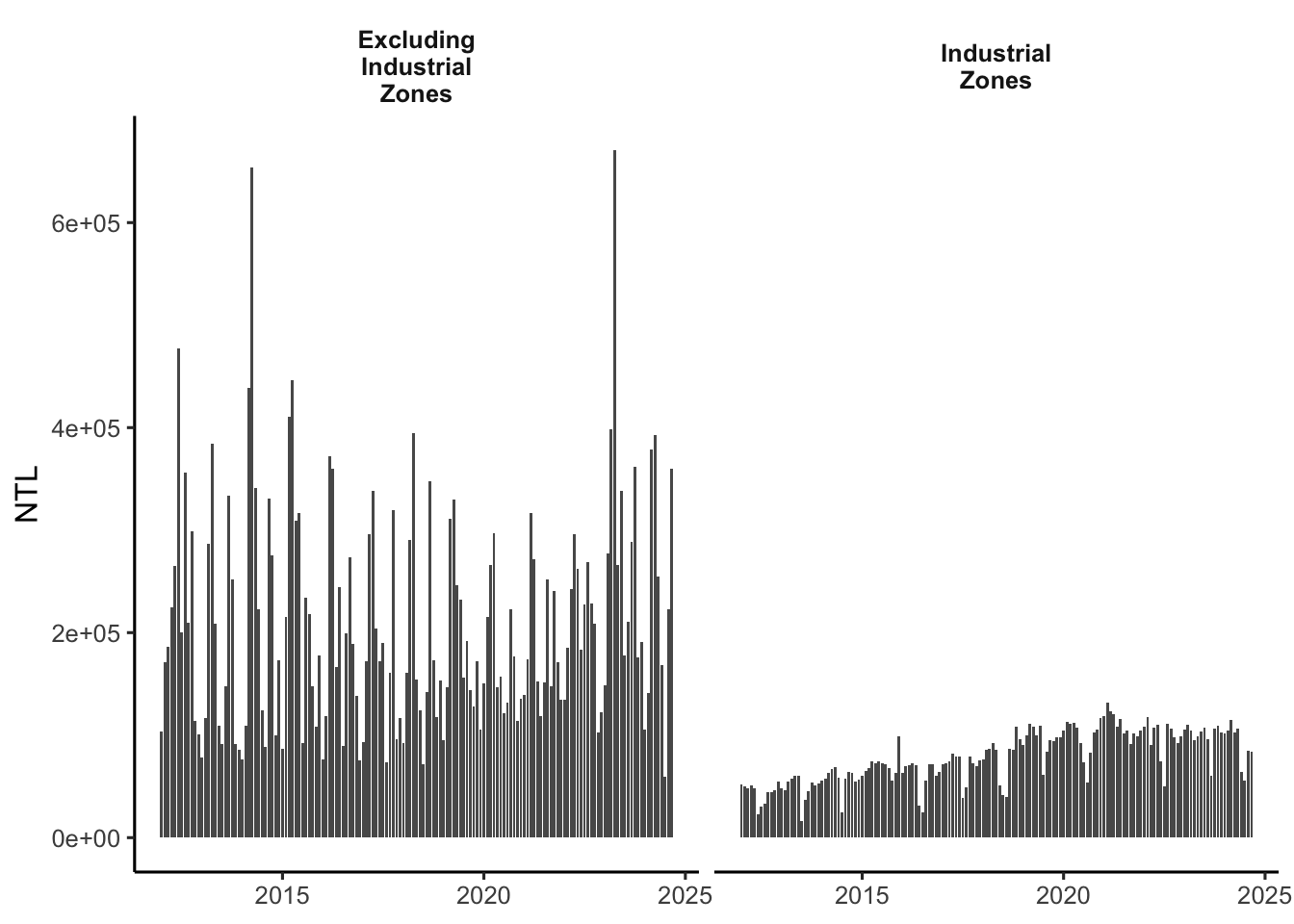
Within different units of analysis (e.g, administrative units) we use the sum of nighttime lights. Where relevant, we distinguish between lights generated from gas flaring and lights removing gas flaring. We use the World Bank’s Global Gas Flaring Tracker which indicates the location of gas flaring locations. When removing gas flaring lights, we remove lights within 10km of a gas flaring location; when looking at lights in gas flaring locations, we take the sum of lights within 10km of gas flaring locations.

Code Setup

Code
#### MAIN PARAMS
proj_dir     <- "~/Dropbox/World Bank/Side Work/Myanmar Economic Monitor Q4"
iso3_code    <- "MMR"
iso2_code    <- "MM"
pc_base_year <- 2019

#### Packages
library(tidyverse)
library(sf)
library(leaflet)
library(leaflet.providers)
library(ggpubr)
library(terra)
library(tidyterra)
library(gtools)
library(readxl)
library(janitor)
library(geodata)
library(exactextractr)
library(blackmarbler)
library(dplyr)
library(readxl)
library(janitor)
library(ggpubr)
library(WDI)
library(kableExtra)
library(elevatr)
library(ggnewscale)
library(pals)
library(haven)

#### Paths

## Define
data_dir       <- file.path(proj_dir, "data")
ntl_bm_dir     <- file.path(data_dir, "Nighttime Lights BlackMarble")
gadm_dir       <- file.path(data_dir, "GADM")
gas_flare_dir  <- file.path(data_dir, "gas-flaring")

## Create
dir.create(proj_dir)
dir.create(data_dir)
dir.create(ntl_bm_dir)
dir.create(gadm_dir)
dir.create(gas_flare_dir)

#### Bearer
nasa_bearer <- read_csv("~/Dropbox/bearer_bm.csv") %>%
  pull(token)

#### Theme
theme_manual <- theme_classic2() +
  theme(strip.background = element_blank(),
        strip.text = element_text(face = "bold"),
        plot.title = element_text(face = "bold"))

#### GADM Boundaries
for(i in 0:2){
  for(iso3_i in iso3_code){
    gadm(iso3_code, level=i, path = file.path(gadm_dir))
  }
} 

#### Load GADM Functions
load_gadm <- function(i){
  roi_sf <- file.path(gadm_dir, 'gadm') %>%
    list.files(full.names = T) %>%
    str_subset(paste0("_",i,"_pk.rds")) %>%
    map_df(function(file_path){
      readRDS(file_path) %>%
        st_as_sf()
    })
}

#### Elevation
dir.create(file.path(data_dir, "elevation"))

OUT_PATH <- file.path(data_dir, "elevation", "elev.tiff")

if(!file.exists(OUT_PATH)){
  
  
  if(length(iso3_code) > 1){
    
    # elev_list <- lapply(iso3_code, function(iso3_code_i){
    #   elevation_3s(country=iso3_code_i, path=tempdir())
    # }) 
    # elev_r <- do.call(mosaic, c(elev_list, fun="mean"))
    
    elev_list <- lapply(iso3_code, function(iso3_code_i){
      
      adm0_sf <- gadm(iso3_code, level=0, path = tempdir())
      get_elev_raster(locations = adm0_sf, z = 8)
      
    })
    elev_r <- do.call(mosaic, c(elev_list, fun="mean"))
    
  } else{
    adm0_sf <- load_gadm(0)
    
    #elev_r <- elevation_3s(country=iso3_code, path=tempdir())
    elev_r <- get_elev_raster(locations = adm0_sf, z = 8)
    
  }
  
  writeRaster(elev_r, OUT_PATH, overwrite = T)
  
}

#### NTL Months to Download
ntl_months <- seq.Date(ymd("2012-01-01"), to = ymd("2024-06-01"), by = "month") %>%
  as.character()

#### Colors
wbg_color_light <- "#1AA1DB"
wbg_color_dark <- "#02224B"

Prep Data

Download Cities

We use a dataset from Geonames which indicates the location of cities with over 1,000 people.

Code
dir.create(file.path(data_dir, "cities"))

## Cities
OUT_FILE_ALL <- file.path(data_dir, "cities", "cities_all.Rds")

if(!file.exists(OUT_FILE_ALL)){
  # https://public.opendatasoft.com/explore/dataset/geonames-all-cities-with-a-population-1000/export/?flg=en-us&disjunctive.cou_name_en&sort=name
  city_df <- read_delim("https://public.opendatasoft.com/api/explore/v2.1/catalog/datasets/geonames-all-cities-with-a-population-1000/exports/csv?lang=en&timezone=America%2FNew_York&use_labels=true&delimiter=%3B", delim = ";")
  
  saveRDS(city_df, OUT_FILE_ALL)
} 

## Country Cities
OUT_FILE_COUNTRY_DF      <- file.path(data_dir, "cities", "cities_country_df.Rds")
OUT_FILE_COUNTRY_SF      <- file.path(data_dir, "cities", "cities_country_sf.Rds")
OUT_FILE_COUNTRY_5K_SF   <- file.path(data_dir, "cities", "cities_country_5km_sf.Rds")
OUT_FILE_COUNTRY_10K_SF  <- file.path(data_dir, "cities", "cities_country_10km_sf.Rds")
OUT_FILE_COUNTRY_BUFF_SF <- file.path(data_dir, "cities", "cities_country_buff_sf.Rds")

if(!file.exists(OUT_FILE_COUNTRY_SF)){
  
  ## Cleanup
  city_country_df <- city_df[city_df$`Country Code` %in% iso2_code,] %>%
    clean_names()
  
  city_country_df <- city_country_df %>%
    separate(coordinates, into = c("lat", "lon"), sep = ",")
  
  ## Spatially Define
  city_country_sf <- city_country_df %>%
    st_as_sf(coords = c("lon", "lat"),
             crs = 4326)
  
  ## Buffer
  city_country_5km_sf <- city_country_sf %>%
    st_buffer(dist = 5000)
  
  city_country_10km_sf <- city_country_sf %>%
    st_buffer(dist = 10000)
  
  ## Dynamic Buffer
  city_country_sf <- city_country_sf %>%
    dplyr::mutate(buffer = case_when(
      population >= 10000000 ~ 30,
      population >= 5000000 ~ 25,
      population >= 1000000 ~ 20,
      population >= 500000 ~ 15,
      population >= 100000 ~ 10,
      TRUE ~ 5
    ))
  
  city_sub_30km_buff_sf <- city_country_sf[city_country_sf$buffer %in% 30,] %>% st_buffer(dist = 30*1000)
  city_sub_25km_buff_sf <- city_country_sf[city_country_sf$buffer %in% 25,] %>% st_buffer(dist = 25*1000)
  city_sub_20km_buff_sf <- city_country_sf[city_country_sf$buffer %in% 20,] %>% st_buffer(dist = 20*1000)
  city_sub_15km_buff_sf <- city_country_sf[city_country_sf$buffer %in% 15,] %>% st_buffer(dist = 15*1000)
  city_sub_10km_buff_sf <- city_country_sf[city_country_sf$buffer %in% 10,] %>% st_buffer(dist = 10*1000)
  city_sub_5km_buff_sf  <- city_country_sf[city_country_sf$buffer %in% 5,]  %>% st_buffer(dist = 5*1000)
  
  city_buff_sf <- bind_rows(city_sub_30km_buff_sf,
                            city_sub_25km_buff_sf,
                            city_sub_20km_buff_sf,
                            city_sub_15km_buff_sf,
                            city_sub_10km_buff_sf,
                            city_sub_5km_buff_sf)
  
  
  ## Export
  saveRDS(city_country_df, OUT_FILE_COUNTRY_DF)
  
  saveRDS(city_country_5km_sf,  OUT_FILE_COUNTRY_5K_SF)
  saveRDS(city_country_10km_sf, OUT_FILE_COUNTRY_10K_SF)
  saveRDS(city_buff_sf,         OUT_FILE_COUNTRY_BUFF_SF)
  saveRDS(city_country_sf,      OUT_FILE_COUNTRY_SF)
  
} 

Download and Append gas flaring

We download and append gas flaring data from the World Bank Global Gas Flaring Database.

Code
dir.create(file.path(gas_flare_dir, "rawdata"))
dir.create(file.path(gas_flare_dir, "finaldata"))

#### Download data
# https://datacatalog.worldbank.org/search/dataset/0037743
if(!file.exists(file.path(gas_flare_dir, "rawdata", "viirs_global_flaring_2017.xlsx"))){
  download.file(url = "https://datacatalogfiles.worldbank.org/ddh-published/0037743/DR0045623/viirs_global_flaring_d.7_slope_0.029353_2017_web_v1.xlsx?versionId=2023-01-18T20:03:32.2273754Z", 
                destfile = file.path(gas_flare_dir, "rawdata", "viirs_global_flaring_2017.xlsx"), 
                mode = "wb")
}

if(!file.exists(file.path(gas_flare_dir, "rawdata", "viirs_global_flaring_2018.xlsx"))){
  download.file(url = "https://datacatalogfiles.worldbank.org/ddh-published/0037743/DR0045622/viirs_global_flaring_d.7_slope_0.029353_2018_web.xlsx?versionId=2023-01-18T20:02:43.3965005Z", 
                destfile = file.path(gas_flare_dir, "rawdata", "viirs_global_flaring_2018.xlsx"), 
                mode = "wb")
}

if(!file.exists(file.path(gas_flare_dir, "rawdata", "viirs_global_flaring_2019.xlsx"))){
  download.file(url = "https://datacatalogfiles.worldbank.org/ddh-published/0037743/DR0045621/viirs_global_flaring_d.7_slope_0.029353_2019_web_v20201114-3.xlsx?versionId=2023-01-18T20:03:09.2456111Z", 
                destfile = file.path(gas_flare_dir, "rawdata", "viirs_global_flaring_2019.xlsx"), 
                mode = "wb")
}

if(!file.exists(file.path(gas_flare_dir, "rawdata", "viirs_global_flaring_2020.xlsx"))){
  download.file(url = "https://datacatalogfiles.worldbank.org/ddh-published/0037743/DR0084248/2020%20Global%20Gas%20Flaring%20Volumes.xlsx?versionId=2023-01-18T20:03:53.8309309Z", 
                destfile = file.path(gas_flare_dir, "rawdata", "viirs_global_flaring_2020.xlsx"), 
                mode = "wb")
}

if(!file.exists(file.path(gas_flare_dir, "rawdata", "viirs_global_flaring_2021.xlsx"))){
  download.file(url = "https://datacatalogfiles.worldbank.org/ddh-published/0037743/DR0087112/2021%20Global%20Gas%20Flaring%20Volumes.xlsx?versionId=2023-01-18T20:02:21.4951166Z", 
                destfile = file.path(gas_flare_dir, "rawdata", "viirs_global_flaring_2021.xlsx"), 
                mode = "wb")
}

#### Append data
clean_data <- function(x){
  x %>% 
    clean_names() %>% 
    dplyr::filter(iso_code %in% iso3_code)
} 

df_2021 <- read_xlsx(file.path(gas_flare_dir, "rawdata", "viirs_global_flaring_2021.xlsx"), 2) %>% clean_data()

df_2020_1 <- read_xlsx(file.path(gas_flare_dir, "rawdata", "viirs_global_flaring_2020.xlsx"), 1) %>% clean_data()
df_2020_2 <- read_xlsx(file.path(gas_flare_dir, "rawdata", "viirs_global_flaring_2020.xlsx"), 2) %>% clean_data()
df_2020_3 <- read_xlsx(file.path(gas_flare_dir, "rawdata", "viirs_global_flaring_2020.xlsx"), 3) %>% clean_data()

df_2019 <- read_xlsx(file.path(gas_flare_dir, "rawdata", "viirs_global_flaring_2019.xlsx"), 1) %>% clean_data()

df_2018_4 <- read_xlsx(file.path(gas_flare_dir, "rawdata", "viirs_global_flaring_2018.xlsx"), 4) %>% clean_data()
df_2018_5 <- read_xlsx(file.path(gas_flare_dir, "rawdata", "viirs_global_flaring_2018.xlsx"), 5) %>% clean_data()
df_2018_6 <- read_xlsx(file.path(gas_flare_dir, "rawdata", "viirs_global_flaring_2018.xlsx"), 6) %>% clean_data()

df_2017_1 <- read_xlsx(file.path(gas_flare_dir, "rawdata", "viirs_global_flaring_2017.xlsx"), 1) %>% clean_data()
df_2017_2 <- read_xlsx(file.path(gas_flare_dir, "rawdata", "viirs_global_flaring_2017.xlsx"), 2) %>% clean_data()
df_2017_3 <- read_xlsx(file.path(gas_flare_dir, "rawdata", "viirs_global_flaring_2017.xlsx"), 3) %>% clean_data()

gs_df <- bind_rows(
  df_2021,
  df_2020_1,
  df_2020_2,
  df_2020_3,
  df_2019,
  df_2018_4,
  df_2018_5,
  df_2018_6,
  df_2017_1,
  df_2017_2,
  df_2017_3
)

gs_df <- gs_df %>%
  dplyr::select(latitude, longitude) %>%
  distinct() %>%
  dplyr::mutate(uid = 1:n())

gs_sf <- gs_df %>% 
  st_as_sf(coords = c("longitude", "latitude"),
           crs = 4326)

gs_5km_sf <- gs_sf %>%
  st_buffer(dist = 5000)

gs_10km_sf <- gs_sf %>%
  st_buffer(dist = 10000)

saveRDS(gs_df, file.path(gas_flare_dir, "finaldata", "gas_flare_locations.Rds"))
saveRDS(gs_5km_sf, file.path(gas_flare_dir, "finaldata", "gas_flare_locations_5km.Rds"))
saveRDS(gs_10km_sf, file.path(gas_flare_dir, "finaldata", "gas_flare_locations_10km.Rds"))

Download Nighttime Lights

Code
#### NTL
roi_sf <- load_gadm(0)

dir.create(file.path(ntl_bm_dir, "rasters"))
dir.create(file.path(ntl_bm_dir, "rasters", "annual"))
dir.create(file.path(ntl_bm_dir, "rasters", "monthly"))

r <- bm_raster(roi_sf = roi_sf,
               product_id = "VNP46A4",
               date = 2012:2023,
               bearer = nasa_bearer,
               output_location_type = "file",
               file_dir = file.path(ntl_bm_dir, "rasters", "annual"))

r <- bm_raster(roi_sf = roi_sf,
               product_id = "VNP46A3",
               date = ntl_months,
               bearer = nasa_bearer,
               output_location_type = "file",
               file_dir = file.path(ntl_bm_dir, "rasters", "monthly"))

Aggregate Nighttime Lights

Code
# Individual Files -------------------------------------------------------------
dir.create(file.path(ntl_bm_dir, "aggregated_individual_files"))

#### Setup loops
for(unit in c("adm0", 
              "adm1", 
              "adm2",
              "mmr_adm0",
              "mmr_adm1",
              "mmr_adm2",
              "mmr_adm3",
              "induszone5km",
              "cities5km",
              "cities10km",
              "citiesbuff")){
  for(time_type in c("annual", "monthly")){
    
    if(time_type == "annual"){
      time_vec <- 2012:2023
    }
    
    if(time_type == "monthly"){
      time_vec <- ntl_months
    }
    
    for(time_i in time_vec){
      
      #### Only process if file doesn't exist
      dir.create(file.path(ntl_bm_dir, "aggregated_individual_files", unit))
      dir.create(file.path(ntl_bm_dir, "aggregated_individual_files", unit, time_type))
      
      OUT_FILE <- file.path(ntl_bm_dir, "aggregated_individual_files", unit, time_type, 
                            paste0("ntl_", time_i, ".Rds"))
      
      if(!file.exists(OUT_FILE)){
        
        #### Load Unit
        if(unit == "adm0"){
          roi_sf <- load_gadm(0)
        }
        
        if(unit == "adm1"){
          roi_sf <- load_gadm(1)
        }
        
        if(unit == "adm2"){
          roi_sf <- load_gadm(2)
        }
        
        if(unit == "mmr_adm0"){
          roi_sf <- read_sf(file.path(data_dir, "Shapefiles", "Boundaries",
                                      "mmr_polbnda_adm0_250k_mimu.shp"))
        }
        
        if(unit == "mmr_adm1"){
          roi_sf <- read_sf(file.path(data_dir, "Shapefiles", "Boundaries",
                                      "mmr_polbnda_adm1_250k_mimu.shp"))
        }
        
        if(unit == "mmr_adm2"){
          roi_sf <- read_sf(file.path(data_dir, "Shapefiles", "Boundaries",
                                      "mmr_polbnda_adm2_250k_mimu_1.shp"))
        }
        
        if(unit == "mmr_adm3"){
          roi_sf <- read_sf(file.path(data_dir, "Shapefiles", "mmr_polbnda_adm3_250k_mimu",
                                      "mmr_polbnda_adm3_250k_mimu.shp"))
        }
        
        if(unit == "induszone5km"){
          roi_sf <- read_sf(file.path(data_dir, "Shapefiles",
                                      "industrial__special_economic_zones_sept2019",
                                      "industrial__special_economic_zones_sept2019.shp"))
          
          roi_sf <- roi_sf %>% st_buffer(dist = 5*1000)
        }
        
        if(unit == "cities5km"){
          roi_sf <- readRDS(file.path(data_dir, "cities", "cities_country_5km_sf.Rds"))
        }
        
        if(unit == "cities10km"){
          roi_sf <- readRDS(file.path(data_dir, "cities", "cities_country_10km_sf.Rds"))
        }
        
        if(unit == "citiesbuff"){
          roi_sf <- readRDS(file.path(data_dir, "cities", "cities_country_buff_sf.Rds"))
        }
        
        #### Load Raster
        if(time_type == "annual"){
          bm_product <- "VNP46A4"
          time_raster_i <- time_i 
        }
        
        if(time_type == "monthly"){
          bm_product <- "VNP46A3"
          
          time_raster_i <- time_i %>% 
            substring(1, 7) %>%
            str_replace_all("-", "_")
        }
        
        ntl_r <- rast(file.path(ntl_bm_dir, "rasters", time_type, 
                                paste0(bm_product,"_NearNadir_Composite_Snow_Free_qflag_t",time_raster_i,".tif")))
        
        #### Gas Flaring Mask
        gs_5km_sf  <- readRDS(file.path(gas_flare_dir, "finaldata", "gas_flare_locations_5km.Rds"))
        gs_10km_sf <- readRDS(file.path(gas_flare_dir, "finaldata", "gas_flare_locations_10km.Rds"))
        
        ntl_gf_5km_r   <- mask(ntl_r, gs_5km_sf)
        ntl_nogf_5km_r <- mask(ntl_r, gs_5km_sf, inverse = T)
        
        ntl_gf_10km_r   <- mask(ntl_r, gs_10km_sf)
        ntl_nogf_10km_r <- mask(ntl_r, gs_10km_sf, inverse = T)
        
        #### Extract NTL
        roi_sf$ntl_sum          <- exact_extract(ntl_r, roi_sf, "sum")
        
        roi_sf$ntl_gf_5km_sum   <- exact_extract(ntl_gf_5km_r, roi_sf, "sum")
        roi_sf$ntl_nogf_5km_sum <- exact_extract(ntl_nogf_5km_r, roi_sf, "sum")
        
        roi_sf$ntl_gf_10km_sum   <- exact_extract(ntl_gf_10km_r, roi_sf, "sum")
        roi_sf$ntl_nogf_10km_sum <- exact_extract(ntl_nogf_10km_r, roi_sf, "sum")
        
        #### Cleanup
        roi_sf$date <- time_i
        
        roi_df <- roi_sf %>%
          st_drop_geometry()
        
        #### Export
        saveRDS(roi_df, OUT_FILE)
        
      }
    }
  }
}

#### Append Files
dir.create(file.path(ntl_bm_dir, "aggregated"))

for(unit in c("adm0", 
              "adm1", 
              "adm2",
              "mmr_adm0",
              "mmr_adm1",
              "mmr_adm2",
              "mmr_adm3",
              "induszone5km",
              "cities5km",
              "cities10km",
              "citiesbuff")){
  for(time_type in c("annual", "monthly")){
    
    ntl_df <- file.path(ntl_bm_dir, "aggregated_individual_files", unit, time_type) %>%
      list.files(full.names = T,
                 pattern = ".Rds") %>%
      map_df(readRDS)
    
    saveRDS(ntl_df,   file.path(ntl_bm_dir, "aggregated", paste0("ntl_", unit, "_", time_type, ".Rds")))
    write_csv(ntl_df, file.path(ntl_bm_dir, "aggregated", paste0("ntl_", unit, "_", time_type, ".csv")))
    write_dta(ntl_df, file.path(ntl_bm_dir, "aggregated", paste0("ntl_", unit, "_", time_type, ".dta")))
    
  }
}

Maps of Nighttime Lights

Interactive Map

Code
#| warning: false
#| message: false

## Load boundaries
adm0_sf <- load_gadm(0)

## Load/prep raster
prep_r <- function(year_i){
  r <- rast(file.path(ntl_bm_dir, "rasters", "annual",
                      paste0("VNP46A4_NearNadir_Composite_Snow_Free_qflag_t",year_i,".tif")))
  r <- r %>% mask(adm0_sf)
  r[][r[] <= 0.05] <- NA
  r[] <- log(r[] + 1)
  #r[] <- log(r[] + 1)
  return(r)
}

r_2012 <- prep_r(2012)
r_2013 <- prep_r(2013)
r_2014 <- prep_r(2014)
r_2015 <- prep_r(2015)
r_2016 <- prep_r(2016)
r_2017 <- prep_r(2017)
r_2018 <- prep_r(2018)
r_2019 <- prep_r(2019)
r_2020 <- prep_r(2020)
r_2021 <- prep_r(2021)
r_2022 <- prep_r(2022)
r_2023 <- prep_r(2023)

## Make map
pal <- colorNumeric(c("black", "yellow", "red"), unique(c(r_2012[],
                                                          r_2013[],
                                                          r_2014[],
                                                          r_2015[],
                                                          r_2016[],
                                                          r_2017[],
                                                          r_2018[],
                                                          r_2019[],
                                                          r_2020[],
                                                          r_2021[],
                                                          r_2022[],
                                                          r_2023[])),
                    na.color = "transparent")

leaflet() %>%
  addProviderTiles(providers$CartoDB.DarkMatter) %>%
  addRasterImage(r_2012, colors = pal, opacity = 1, group = "2012") %>%
  addRasterImage(r_2013, colors = pal, opacity = 1, group = "2013") %>%
  addRasterImage(r_2014, colors = pal, opacity = 1, group = "2014") %>%
  addRasterImage(r_2015, colors = pal, opacity = 1, group = "2015") %>%
  addRasterImage(r_2016, colors = pal, opacity = 1, group = "2016") %>%
  addRasterImage(r_2017, colors = pal, opacity = 1, group = "2017") %>%
  addRasterImage(r_2018, colors = pal, opacity = 1, group = "2018") %>%
  addRasterImage(r_2019, colors = pal, opacity = 1, group = "2019") %>%
  addRasterImage(r_2020, colors = pal, opacity = 1, group = "2020") %>%
  addRasterImage(r_2021, colors = pal, opacity = 1, group = "2021") %>%
  addRasterImage(r_2022, colors = pal, opacity = 1, group = "2022") %>%
  addRasterImage(r_2023, colors = pal, opacity = 1, group = "2023") %>%
  addLayersControl(
    baseGroups = paste0(2012:2023),
    options = layersControlOptions(collapsed=FALSE)
  )

Static Map of Nighttime Lights

Code
## Load boundaries
adm0_sf <- load_gadm(0)

## Elevation
elev_r <- rast(file.path(data_dir, "elevation", "elev.tiff"))
slope_r <- terrain(elev_r)
slope_r <- slope_r %>% mask(adm0_sf)

## Latest Year
r <- rast(file.path(ntl_bm_dir, "rasters", "annual",
                    paste0("VNP46A4_NearNadir_Composite_Snow_Free_qflag_t",2023,".tif")))
r <- r %>% mask(adm0_sf)

r[][r[] <= 1] <- NA
r[] <- log(r[] + 1)
r[] <- log(r[] + 1)

ocean_colors <- ocean.deep(100)
ocean_colors[98:100] <- "#FFFFFF"

ggplot() +
  geom_spatraster(data = slope_r, 
                  show.legend = FALSE,
                  maxcell = 9e+07) +
  scale_fill_gradient(low = "#49232E",
                      high = "black",
                      na.value = "transparent") +
  ggnewscale::new_scale_fill() +
  geom_spatraster(data = r,
                  aes(fill = t2023),
                  maxcell = 9e+07) +
  scale_fill_gradientn(colors = ocean_colors,
                       #midpoint = 2,
                       na.value = "transparent") +
  labs(fill = "Light Intensity",
       title = "Nighttime Lights",
       subtitle = 2023) +
  coord_sf() +
  theme_void() +
  theme(plot.title = element_text(face = "bold", hjust = 0.5, size = 16),
        plot.subtitle = element_text(face = "italic", hjust = 0.5, size = 16),
        legend.position = c(0.2, 0.15)) +
  guides(fill = guide_colorbar(direction = "horizontal",
                               label = FALSE,         
                               title.position = "top"))

Diagnostics

Nighttime Lights: Gas Flaring vs Non Gas Flaring

Trend Figure

Code
ntl_df <- readRDS(file.path(ntl_bm_dir, "aggregated", "ntl_adm0_annual.Rds"))

ntl_df %>%
  dplyr::select(date, ntl_gf_10km_sum, ntl_nogf_10km_sum) %>%
  pivot_longer(cols = -date) %>%
  dplyr::mutate(name = case_when(
    name == "ntl_nogf_10km_sum" ~ "NTL: No Gas Flares",
    name == "ntl_gf_10km_sum" ~ "NTL: Gas Flares"
  )) %>%
  
  ggplot() +
  geom_col(aes(x = date,
               y = value,
               fill = name),
           stat = "identity", position = 'dodge') +
  labs(fill = NULL,
       x = NULL,
       y = "NTL") +
  scale_fill_manual(values = c(wbg_color_light,
                               wbg_color_dark)) +
  theme_manual

Percent of NTL from Gas Flaring

Code
ntl_df <- readRDS(file.path(ntl_bm_dir, "aggregated", "ntl_adm0_annual.Rds"))

ntl_df %>%
  dplyr::mutate(per_gf = (ntl_gf_10km_sum / ntl_sum) * 100) %>%
  dplyr::select(date, COUNTRY, per_gf) %>%
  pivot_wider(id_cols = date,
              names_from = COUNTRY,
              values_from = per_gf) %>%
  dplyr::rename(Year = date) %>%
  kable()
Year Myanmar
2012 0.1752236
2013 0.2707532
2014 0.2418248
2015 0.2095962
2016 0.1609097
2017 0.1757831
2018 0.1325673
2019 0.1476140
2020 0.1625885
2021 0.1624325
2022 0.1886330
2023 0.2171269

NTL vs City Population

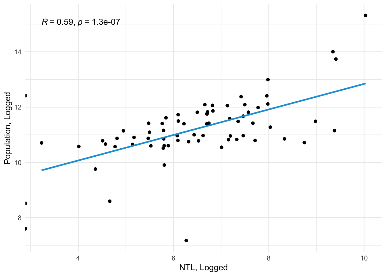
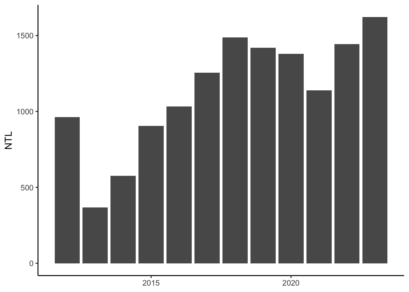
We use a dataset from [Geonames] that maps the locations of all cities with other 1,000 people. We extract total nighttime lights withing a 5km buffer of each city. The below figure compares nighttime lights with population.

Code
city_df <- readRDS(file.path(data_dir, "cities", "cities_country_df.Rds"))
city_df <- city_df %>%
  dplyr::select(geoname_id, lat, lon)

ntl_df <- readRDS(file.path(ntl_bm_dir, "aggregated", 
                            paste0("ntl_", "citiesbuff", "_", "annual", ".Rds")))

ntl_coord_df <- ntl_df %>%
  dplyr::filter(date == 2023) %>%
  left_join(city_df, by = "geoname_id") %>%
  dplyr::mutate(lat = lat %>% as.numeric(),
                lon = lon %>% as.numeric()) %>%
  arrange(ntl_sum)

adm0_sf <- load_gadm(0)

ntl_df %>%
  ggplot() +
  geom_sf(data = adm0_sf) +
  geom_point(data = ntl_coord_df,
             aes(x = lon, 
                 y = lat,
                 fill = log(ntl_sum),
                 size = ntl_sum),
             pch = 21,
             color = "black") +
  labs(size = "Nighttime\nLights",
       title = "Nighttime Lights Across Cities") +
  theme_void() +
  theme(plot.title = element_text(face = "bold", hjust = 0.5)) +
  scale_fill_gradient(low = wbg_color_dark,
                      high = wbg_color_light) +
  guides(fill = "none")

Code
ntl_df <- readRDS(file.path(ntl_bm_dir, "aggregated", 
                            paste0("ntl_", "cities10km", "_", "annual", ".Rds")))

ntl_df %>%
  dplyr::filter(population > 0,
                date == 2023) %>%
  ggplot(aes(x = log(ntl_sum),
             y = log(population))) +
  geom_point(fill = wbg_color_dark) +
  geom_smooth(method=lm, 
              se=FALSE,
              color = wbg_color_light) +
  stat_cor() +
  theme_minimal() +
  labs(x = "NTL, Logged",
       y = "Population, Logged")

Nighttime Lights as Proxy for GDP

Code
# Download GDP
dir.create(file.path(data_dir, "wdi"))
OUT_FILE <- file.path(data_dir, "wdi", "gdp.Rds")

if(!file.exists(OUT_FILE)){
  gdp_df <- WDI(indicator = c("NY.GDP.PCAP.CD",
                              "NY.GDP.MKTP.CD"), 
                country = iso3_code, 
                start = 2012, 
                end = 2023)
  
  saveRDS(gdp_df, OUT_FILE)
} else{
  gdp_df <- readRDS(OUT_FILE)
}

# Correlation with GDP
ntl_df <- readRDS(file.path(ntl_bm_dir, "aggregated", 
                            paste0("ntl_", "adm0", "_", "annual", ".Rds")))

ntl_df <- ntl_df %>%
  dplyr::rename(year = date)

# Filter
if(paste(iso3_code, collapse = ";") %in% "SSD;SDN"){
  ntl_df <- ntl_df[ntl_df$COUNTRY %in% "Sudan",]
  gdp_df <- gdp_df[gdp_df$country %in% "Sudan",]
}

ntl_gdp_df <- ntl_df %>%
  left_join(gdp_df, by = "year") %>%
  clean_names()

## Line Plots
ntl_gdp_df %>%
  dplyr::select(year, 
                ntl_sum,
                ntl_gf_10km_sum,
                ntl_nogf_10km_sum,
                ny_gdp_pcap_cd,
                ny_gdp_mktp_cd) %>%
  pivot_longer(cols = -year) %>%
  dplyr::mutate(name = case_when(
    name == "ntl_sum" ~ "Nighttime Lights",
    name == "ntl_gf_10km_sum" ~ "Nighttime Lights:\nGas Flares",
    name == "ntl_nogf_10km_sum" ~ "Nighttime Lights:\nNo Gas Flares",
    name == "ny_gdp_pcap_cd" ~ "GDP, Per Capita",
    name == "ny_gdp_mktp_cd" ~ "GDP"
  )) %>%
  dplyr::mutate(type = name %>% str_detect("GDP")) %>%
  ggplot(aes(x = year,
             y = value,
             color = type)) +
  geom_line(linewidth = 1) +
  facet_wrap(~name,
             scales = "free_y") +
  labs(x = NULL,
       y = NULL) +
  scale_color_manual(values = c(wbg_color_light, wbg_color_dark)) +
  theme_manual +
  theme(legend.position = "none")

Code
## Correlation: GDP
ntl_gdp_df %>%
  dplyr::select(ntl_sum, 
                ntl_gf_10km_sum,
                ntl_nogf_10km_sum,
                ny_gdp_mktp_cd) %>%
  pivot_longer(cols = -c(ny_gdp_mktp_cd)) %>%
  dplyr::mutate(name = case_when(
    name == "ntl_sum" ~ "NTL",
    name == "ntl_gf_10km_sum" ~ "NTL: Gas Flare",
    name == "ntl_nogf_10km_sum" ~ "NTL: No Gas Flare",
  )) %>%
  
  ggplot(aes(x = value,
             y = ny_gdp_mktp_cd)) +
  geom_point() +
  geom_smooth(method=lm, 
              se=FALSE,
              color = wbg_color_light) +
  stat_cor() +
  labs(x = "NTL",
       y = "GDP",
       title = "Correlation of Nighttime Lights with GDP") +
  facet_wrap(~name,
             scales = "free") +
  theme_manual 

Code
## Correlation: GDP
ntl_gdp_df %>%
  dplyr::select(ntl_sum, 
                ntl_gf_10km_sum,
                ntl_nogf_10km_sum,
                ny_gdp_pcap_cd) %>%
  pivot_longer(cols = -c(ny_gdp_pcap_cd)) %>%
  dplyr::mutate(name = case_when(
    name == "ntl_sum" ~ "NTL",
    name == "ntl_gf_10km_sum" ~ "NTL: Gas Flare",
    name == "ntl_nogf_10km_sum" ~ "NTL: No Gas Flare",
  )) %>%
  
  ggplot(aes(x = value,
             y = ny_gdp_pcap_cd)) +
  geom_point() +
  geom_smooth(method=lm, 
              se=FALSE,
              color = wbg_color_light) +
  stat_cor() +
  labs(x = "NTL",
       y = "GDP, per Capita",
       title = "Correlation of Nighttime Lights with per Capita GDP") +
  facet_wrap(~name,
             scales = "free") +
  theme_manual

% Change Maps

ADM 1

Code
## Load
adm_sf <- load_gadm(1)
ntl_df <- readRDS(file.path(ntl_bm_dir, "aggregated", "ntl_adm1_annual.Rds"))

## Prep data
ntl_wide_df <- ntl_df %>%
  dplyr::filter(date %in% c(pc_base_year:2023)) %>%
  dplyr::select(GID_1, date, ntl_sum) %>%
  dplyr::mutate(date = paste0("yr", date)) %>%
  pivot_wider(names_from = date,
              values_from = ntl_sum,
              id_cols = GID_1)

ntl_wide_df$base_year <- ntl_wide_df[[paste0("yr", pc_base_year)]]

ntl_wide_df <- ntl_wide_df %>%
  dplyr::mutate(pc20 = (yr2020 - base_year)/base_year * 100,
                pc21 = (yr2021 - base_year)/base_year * 100,
                pc22 = (yr2022 - base_year)/base_year * 100,
                pc23 = (yr2023 - base_year)/base_year * 100)

## Map
adm_data_sf <- adm_sf %>%
  left_join(ntl_wide_df, by = "GID_1") %>%
  pivot_longer(cols = c(pc20, pc21, pc22, pc23)) %>%
  dplyr::mutate(name = case_when(
    name == "pc20" ~ paste0("% Change: ",pc_base_year," to 2020"),
    name == "pc21" ~ paste0("% Change: ",pc_base_year," to 2021"),
    name == "pc22" ~ paste0("% Change: ",pc_base_year," to 2022"),
    name == "pc23" ~ paste0("% Change: ",pc_base_year," to 2023")
  ))

adm_data_sf$value[adm_data_sf$value >= 100] <- 100
adm_data_sf$value[adm_data_sf$value <= -100] <- -100

ggplot() +
  geom_sf(data = adm_data_sf,
          aes(fill = value)) +
  facet_wrap(~name) +
  labs(fill = "% Change") +
  scale_fill_gradient2(low = "red",
                       mid = "white",
                       high = "forestgreen",
                       midpoint = 0,
                       limits = c(-100, 100),
                       breaks = c(-100, -50, 0, 50, 100),
                       labels = c("< -100", "-50", "0", "50", "> 100")) +
  theme_manual +
  theme_void() +
  theme(strip.text = element_text(face = "bold"))

ADM 2

Code
## Load
adm_sf <- load_gadm(2)
ntl_df <- readRDS(file.path(ntl_bm_dir, "aggregated", "ntl_adm2_annual.Rds"))

## Prep data
ntl_wide_df <- ntl_df %>%
  dplyr::filter(date %in% c(pc_base_year:2023)) %>%
  dplyr::select(GID_2, date, ntl_sum) %>%
  dplyr::mutate(date = paste0("yr", date)) %>%
  pivot_wider(names_from = date,
              values_from = ntl_sum,
              id_cols = GID_2)

ntl_wide_df$base_year <- ntl_wide_df[[paste0("yr", pc_base_year)]]

ntl_wide_df <- ntl_wide_df %>%
  dplyr::mutate(pc20 = (yr2020 - base_year)/base_year * 100,
                pc21 = (yr2021 - base_year)/base_year * 100,
                pc22 = (yr2022 - base_year)/base_year * 100,
                pc23 = (yr2023 - base_year)/base_year * 100)

## Map
adm_data_sf <- adm_sf %>%
  left_join(ntl_wide_df, by = "GID_2") %>%
  pivot_longer(cols = c(pc20, pc21, pc22, pc23)) %>%
  dplyr::mutate(name = case_when(
    name == "pc20" ~ paste0("% Change: ",pc_base_year," to 2020"),
    name == "pc21" ~ paste0("% Change: ",pc_base_year," to 2021"),
    name == "pc22" ~ paste0("% Change: ",pc_base_year," to 2022"),
    name == "pc23" ~ paste0("% Change: ",pc_base_year," to 2023")
  ))

adm_data_sf$value[adm_data_sf$value >= 100] <- 100
adm_data_sf$value[adm_data_sf$value <= -100] <- -100

ggplot() +
  geom_sf(data = adm_data_sf,
          aes(fill = value)) +
  facet_wrap(~name) +
  labs(fill = "% Change") +
  scale_fill_gradient2(low = "red",
                       mid = "white",
                       high = "forestgreen",
                       midpoint = 0,
                       limits = c(-100, 100),
                       breaks = c(-100, -50, 0, 50, 100),
                       labels = c("< -100", "-50", "0", "50", "> 100")) +
  theme_manual +
  theme_void() +
  theme(strip.text = element_text(face = "bold"))

Industrial Zones

Annual

Code
ntl_df <- readRDS(file.path(ntl_bm_dir, "aggregated", "ntl_induszone5km_annual.Rds"))

ntl_df %>%
  group_by(date) %>%
  dplyr::summarise(ntl_sum = sum(ntl_sum, na.rm = T)) %>%
  ungroup() %>%
  
  ggplot() +
  geom_col(aes(x = date,
               y = ntl_sum))

Monthly

Code
ntl_df <- readRDS(file.path(ntl_bm_dir, "aggregated", "ntl_induszone5km_monthly.Rds"))

ntl_df %>%
  mutate(date = date %>% ymd()) %>%
  group_by(date) %>%
  dplyr::summarise(ntl_sum = sum(ntl_sum, na.rm = T)) %>%
  ungroup() %>%
  
  ggplot() +
  geom_col(aes(x = date,
               y = ntl_sum))

Conflict vs Non Conflict Locations

Code
## Load
ntl_df <- readRDS(file.path(ntl_bm_dir, "aggregated", "ntl_mmr_adm3_annual.Rds"))

acled_1_df <- read_dta(file.path(data_dir, "Conflict", 
                                 "ACLED_01_Jan_2021_21_Oct_2024_township_monthly_spatial.dta"))

acled_2_df <- read_dta(file.path(data_dir, "Conflict", 
                                 "ACLED_Apr_2022_Sep_2024_township_spatial_period_change.dta"))

## Cleanup
base_date <- ymd("1960-01-01")
acled_1_df$date_ymd <- base_date %m+% months(acled_1_df$month)

## Limit variables
ntl_df <- ntl_df %>%
  dplyr::select(TS_PCODE, date, ntl_sum)

acled_1_df <- acled_1_df %>%
  dplyr::select(TS_PCODE, date_ymd, conflict_index, conflict_category) %>%
  dplyr::rename(date = date_ymd)

acled_2_df <- acled_2_df %>%
  dplyr::select(TS_PCODE, 
                apr2022sep2022, 
                oct2022mar2023,
                apr2023sep2023,
                oct2023mar2024,
                apr2024sep2024,
                change1,
                change2,
                compared_to_past_6_months,
                compared_to_last_year)

#### Conflict indicator
conflict_df <- acled_1_df %>%
  group_by(TS_PCODE) %>%
  dplyr::summarise(conflict_category = max(conflict_category)) %>%
  ungroup()

#### Merge
ntl_conf_df <- ntl_df %>%
  left_join(conflict_df, by = "TS_PCODE") %>%
  dplyr::mutate(conflict_category_fct = conflict_category %>% as_factor())

ntl_conf_agg_df <- ntl_conf_df %>%
  group_by(date, conflict_category_fct) %>%
  dplyr::summarise(ntl_sum = mean(ntl_sum)) %>%
  ungroup() 

ntl_conf_agg_df %>%
  ggplot() +
  geom_line(aes(x = date,
                y = ntl_sum,
                color = conflict_category_fct)) +
  labs(color = NULL,
       y = "NTL Radiance",
       x = NULL) +
  theme_classic2()

Code
ntl_conf_agg_df %>%
  ggplot() +
  geom_line(aes(x = date,
                y = ntl_sum)) +
  facet_wrap(~conflict_category_fct) +
  labs(color = NULL,
       y = "NTL Radiance",
       x = NULL) +
  theme_classic2()