Introduction to Dask and the Open Data Cube

Prerequisites: This material assumes basic knowledge of the Open Data Cube, Xarray and numerical processing using numpy.

• Introduction
  • Planning and writing efficient applications
  • What you will learn
• Performance in Python
  • Python list and numpy
  • Numba - accelerating Python
• Parallelism with Dask
  • Review of dask
  • Dask local cluster

The Open Data Cube library is written in Python and makes extensive use of scientific and geospatial libraries. For the purposes of this tutorial we will primarily consider five libraries:

1. datacube - EO datacube
2. xarray - labelled arrays
3. (optional) dask & distributed - distributed parallel programming
4. numpy - numerical array processing with vectorisation
5. (optional) numba - a library for high performance python

Whilst the interrelations are intimate it is useful to conceptualise them according to their primary role and how these roles build from low level numerical array processing (numpy) through to high-level EO datacube semantics (datacube and xarray). If you prefer, viewed from top to bottom we can say:

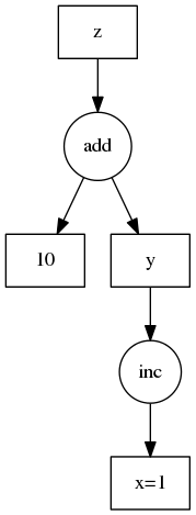
1. datacube.load() does the necessary file IO and data manipulation to construct a...
2. xarray which will be labelled with the necessary coordinate systems and band names and made up of...
3. (optionally) dask.arrays which contain many chunks which are...
4. numpy arrays containing the actual data values.

Each higher level of abstraction thus builds on the lower level components that perform the actual storage and computation.

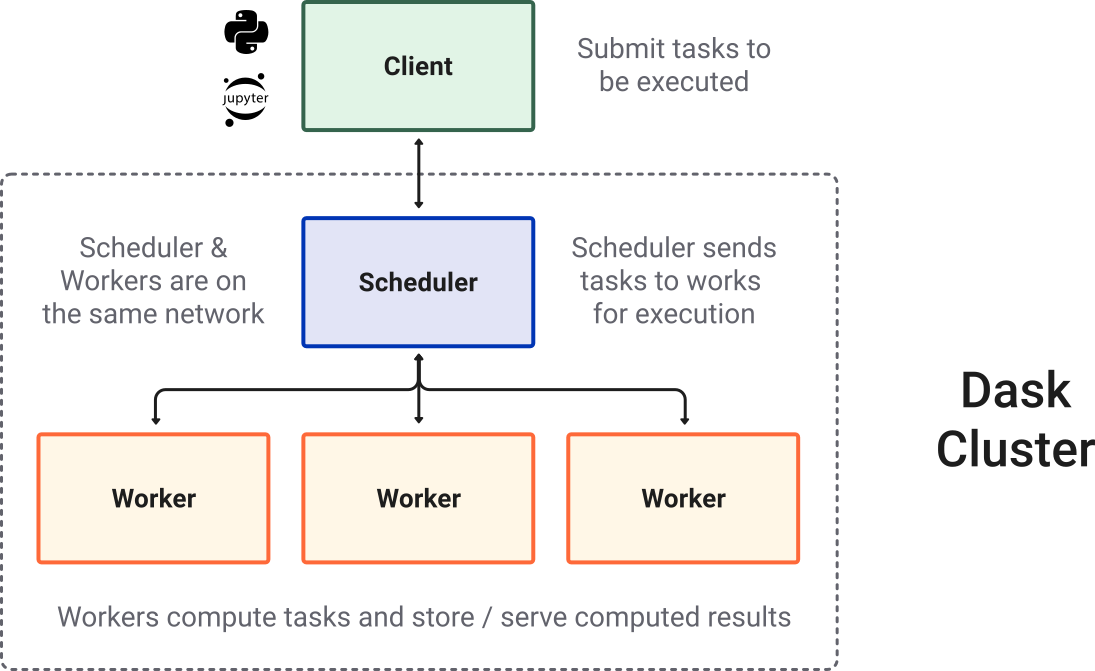
Overlaid on this are libraries like numba, dask and distributed that provide computational components that can accelerate and distribute processing across multiple compute cores and computers. The use of dask, distributed and numba are optional - not all applications require the additional complexity of these tools.

Planning and writing efficient applications

Achieving performance and scale requires an understanding of the performance of each library and how it interacts with the others. Moreover, and often counterintuitively, adding more compute cores to a problem may not make it faster; in fact it may slow down (as well as waste resources). Added to that is the deceptive simplicity in that some of the tools can be simply turned on with only a few code changes and significant performance increases can be achieved.

However, as the application is scaled or an alternative algorithm is used further challenges may arise, in expected I/O or compute efficiency, that require code refactors and changes in algorithmic approach. These challenges can seem to undo some of the earlier work and be frustrating to address.

The good news is whilst there is complexity (six interrelated libraries mentioned so far), there are common concepts and techniques involved in analysing how to optimise your algorithm. If you know from the start your application is going to require scale, then it does help to think in advance where you are heading.

What you will learn

This course will equip readers with concepts and techniques they can utilise in their algorithm and workflow development. The course will be using computer science terms and a variety of libraries but won't be discussing these in detail in order to keep this course concise. The focus will be on demonstration by example and analysis techniques to identify where to focus effort. The reader is encouraged to use their favorite search engine to dig deeper when needed; there are a lot of tutorials online!

One last thing, in order to maintain a healthy state of mind for "Dask and ODC", the reader is encouraged to hold both of these truths in mind at the same time:

1. The best thing about dask is it makes distributed parallel programming in the datacube easy
2. The worst thing about dask it is makes distributed parallel programming in the datacube easy

Yep, that's contradictory! By the end of this course, and a couple of your own adventures, you will understand why.

# EASI defaults
import git
import sys
import os
os.environ['USE_PYGEOS'] = '0'
repo = git.Repo('.', search_parent_directories=True).working_tree_dir
if repo not in sys.path: sys.path.append(repo)
from easi_tools import EasiDefaults, notebook_utils

easi = EasiDefaults()

Successfully found configuration for deployment "csiro"

Performance in Python

In this section we will explore python performance for array processing. Python itself, as you will soon see, is quite slow. It is, however, highly expressive and can orchestrate more complex and faster libraries of numerical code (e.g., numpy). Python is also ammendable to being accelerated (e.g. using numba) and made to run on multiple CPU cores (e.g. via dask).

Python list and numpy

Let's take a look at the simple addition of two arrays. In Python the nearest data type to an array is a list of numbers. This will be our starting point.

Our focus is on performance so we'll use the Jupyter %%time and %%timeit magics to run our cells and time their execution. The latter will run the cell multiple times and provide us with more representative statistics of performance and variability.

First in pure Python using lists :

size_of_vec = 2000*2000
X_list = range(size_of_vec)
Y_list = range(size_of_vec)

%%timeit -n 10 -r 1
Z = [X_list[i] + Y_list[i] for i in range(len(X_list)) ]

967 ms ± 0 ns per loop (mean ± std. dev. of 1 run, 10 loops each)

Now the same processing using numpy.

import numpy
X = numpy.arange(size_of_vec)
Y = numpy.arange(size_of_vec)

%%timeit -n 10 -r 1
Z = X + Y

8.93 ms ± 0 ns per loop (mean ± std. dev. of 1 run, 10 loops each)

Let's check that the two arrays are identical (note that %%timeit does not make the variables above available due to the way that %%timeit works, so we reconstruct the arrays).

print("Are the arrays identical?")
([X_list[i] + Y_list[i] for i in range(len(X_list)) ] == X + Y).all()

Are the arrays identical?

True

At least two orders of magnitude in performance improvement!

Why?

numpy provides a python interface to an underlying C array library that makes use of CPU vectorization - this allows it to process several add operations at the same time.

numpy isn't the only library that does this type of wrapping over a fast optimised library. There are, for example,

• cuPy which uses GPUs for array processing
• tensorflow uses both CPU and GPU optimisations for machine learning
• datashader for large dataset visualisation

It's a very long list and thanks to a great deal of work by a great many software engineers most of these libraries will work together efficiently.

Tip: Where possible use high performance libraries that have python wrappers.

The reader will have noticed the change in abstraction. The pure Python version used list comprehension syntax to add the two arrays, while numpy was a much shorter direct addition syntax more in keeping with the mathematics involved. This change in abstraction is seen in most libraries, including the ODC library where datacube.load() is shorthand for a complex process of data discovery, reprojection, fusing and array construction. High-level abstractions like this are powerful and greatly simplify development (the good). They can also hide performance bottlenecks and challenges (the bad).

Tip: Use high level API abstractions but be mindful of their use.

Numba - accelerating Python

So high performance libraries rock, but what if you don't have one for your purpose and you're back in Python? Numba translates Python functions into optimized machine code at runtime - https://numba.pydata.org.

Let's see how this works. A more complex example this time with a smoothing function applied over our (random) image, perform an FFT, and save the result. These examples are (very) slightly modified versions from the High Performance Python Processing Pipeline video by Matthew Rocklin. It's such a good introduction its worth repeating.

We'll also use the tqdm library to provide a progress bar.

import numpy as np
from tqdm.notebook import tqdm

def load_eo_data():
    return np.random.random((1000, 1000))

def smooth(x):
    out = np.empty_like(x)
    for i in range(1, x.shape[0] - 1):
        for j in range(1, x.shape[1] - 1):
            out[i, j] = (x[i + -1, j + -1] + x[i + -1, j + 0] + x[i + -1, j + 1] +
                         x[i +  0, j + -1] + x[i +  0, j + 0] + x[i +  0, j + 1] +
                         x[i +  1, j + -1] + x[i +  1, j + 0] + x[i +  1, j + 1]) // 9
    return out

def save(x, filename):
    pass 

%%time
for i in tqdm(range(5)):
    img = load_eo_data()
    img = smooth(img)
    img = np.fft.fft2(img)
    save(img, "file-" + str(i) + "-.dat")

  0%|          | 0/5 [00:00<?, ?it/s]

CPU times: user 10.7 s, sys: 11.1 ms, total: 10.7 s
Wall time: 10.7 s

The smooth(x) function contains two python loops. Now we could (and would) find a similar high performance library with a smooth(x) function but for this example let's use numba's jit compiler to translate the python function into optimized machine code at runtime.

import numba

fast_smooth  = numba.jit(smooth)

%%time

for i in tqdm(range(5)):
    img = load_eo_data()
    img = fast_smooth(img)
    img = np.fft.fft2(img)
    save(img, "file-" + str(i) + "-.dat")

  0%|          | 0/5 [00:00<?, ?it/s]

CPU times: user 1.45 s, sys: 19.7 ms, total: 1.47 s
Wall time: 1.46 s

Just a bit quicker! Much of the time in the first run was numba performing compilation. Run the cell above again and you'll find it runs faster the second time.

The recommended approach to have numba compile a python function is to use python decorator syntax (@numba.jit). So the original code now looks like this (single line changed) and we can call smooth(x) without having to create fast_smooth:

import numpy as np

def load_eo_data():
    return np.random.random((1000, 1000))

@numba.jit
def smooth(x):
    out = np.empty_like(x)
    for i in range(1, x.shape[0] - 1):
        for j in range(1, x.shape[1] - 1):
            out[i, j] = (x[i + -1, j + -1] + x[i + -1, j + 0] + x[i + -1, j + 1] +
                         x[i +  0, j + -1] + x[i +  0, j + 0] + x[i +  0, j + 1] +
                         x[i +  1, j + -1] + x[i +  1, j + 0] + x[i +  1, j + 1]) // 9
    return out

def save(x, filename):
    pass

%%time
for i in tqdm(range(5)):
    img = load_eo_data()
    img = smooth(img)
    img = np.fft.fft2(img)
    save(img, "file-" + str(i) + "-.dat")

  0%|          | 0/5 [00:00<?, ?it/s]

CPU times: user 1.16 s, sys: 4.12 ms, total: 1.16 s
Wall time: 1.16 s

Why not use numba all the time everywhere?

Like most high level abstractions numba makes assumption about code, only accelerates a subset of python libraries (not all numpy functions are available via numba), and it is entirely possible it can make performance worse or not work at all!

There's one additional consideration. If you've run all the cells to this point in order, try running the fast_smooth cell again, repeated below for convenience:

fast_smooth  = numba.jit(smooth)

---------------------------------------------------------------------------
TypeError                                 Traceback (most recent call last)
Cell In[14], line 1
----> 1 fast_smooth  = numba.jit(smooth)

File /env/lib/python3.10/site-packages/numba/core/decorators.py:179, in jit(signature_or_function, locals, cache, pipeline_class, boundscheck, **options)
    176 wrapper = _jit(sigs, locals=locals, target=target, cache=cache,
    177                targetoptions=options, **dispatcher_args)
    178 if pyfunc is not None:
--> 179     return wrapper(pyfunc)
    180 else:
    181     return wrapper

File /env/lib/python3.10/site-packages/numba/core/decorators.py:191, in _jit.<locals>.wrapper(func)
    189 def wrapper(func):
    190     if extending.is_jitted(func):
--> 191         raise TypeError(
    192             "A jit decorator was called on an already jitted function "
    193             f"{func}.  If trying to access the original python "
    194             f"function, use the {func}.py_func attribute."
    195         )
    197     if not inspect.isfunction(func):
    198         raise TypeError(
    199             "The decorated object is not a function (got type "
    200             f"{type(func)})."
    201         )

TypeError: A jit decorator was called on an already jitted function CPUDispatcher(<function smooth at 0x7f7c3b220700>).  If trying to access the original python function, use the CPUDispatcher(<function smooth at 0x7f7c3b220700>).py_func attribute.

Error!

The smooth function was decorated so is already jit-compiled. Attempting to do so again causes this error, and exposes some of the low level changes behind the abstraction. This can make debugging code difficult if you are not mindful of what is occuring.

TIP: Use high level API abstractions but be mindful of their use

Parallelism with Dask

Our fake EO processing pipeline only has 5 images and takes about 1 sec to run. In practice we'll have 1000s of images to process (if not more).

Let's repeat our example code but now with more iterations. You can understand why we use The tqdm library to provide a progress bar for these larger scale examples rather than printing out each iteration number or staring at a blank screen wondering if it works!

import numpy as np
import numba
from tqdm.notebook import tqdm


def load_eo_data():
    return np.random.random((1000, 1000))

@numba.jit
def smooth(x):
    out = np.empty_like(x)
    for i in range(1, x.shape[0] - 1):
        for j in range(1, x.shape[1] - 1):
            out[i, j] = (x[i + -1, j + -1] + x[i + -1, j + 0] + x[i + -1, j + 1] +
                         x[i +  0, j + -1] + x[i +  0, j + 0] + x[i +  0, j + 1] +
                         x[i +  1, j + -1] + x[i +  1, j + 0] + x[i +  1, j + 1]) // 9
    return out

def save(x, filename):
    pass

Before running the next code, open a terminal window (File>New>Terminal) and run htop at the command line to show current CPU usage per core.

TIP: Drag your terminal window so that it sits below this notebook before you run htop to see both windows at the same time.

%%time
for i in tqdm(range(1000)):
    img = load_eo_data()
    img = smooth(img)
    img = np.fft.fft2(img)
    save(img, "file-" + str(i) + "-.dat")

  0%|          | 0/1000 [00:00<?, ?it/s]

CPU times: user 45.3 s, sys: 60.3 ms, total: 45.3 s
Wall time: 45.2 s

You'll notice that only one core is showing any load. The above code is not using any of the additional cores.

dask can be useful in this scenario even on a local machine.

Review of dask

Firstly, a few notes on terminology. A Dask Cluster is comprised of a client, a scheduler, and workers. These terms will be used throughout this tutorial. Figure 1 below shows the relationship between each of these components. The client submits tasks to the scheduler, which decides how to submit the tasks to individual workers. During this process, the scheduler creates what is called a Task Graph. This is essentially a map of the tasks that need to be carried out. Figure 2 shows an example of a simple task graph (see https://docs.dask.org/en/stable/graphs.html for more information). Workers carry out the actual calculations and either store the results or send them back to the client.

Figure 1. Overview of a Dask Cluster.

Figure 2. A simple Task Graph.

Dask has several core data types, including Dask DataFrames and Dask Arrays. Essentially, Dask DataFrames are parallelized Pandas DataFrames (Figure 3) and Dask Arrays are parallelized Numpy arrays (Figure 4).

Figure 3. A Dask DataFrame is comprised of many in-memory pandas DataFrames separated along an index.

Figure 4. A Dask Array is a subset of the NumPy ndarray interface using blocked algorithms, cutting up the large array into many small arrays.

EASI and the Open Data Cube primarily make use of Dask DataArrays. For more information see https://tutorial.dask.org/02_array.html.

Dask local cluster

Let's start by creating a local dask cluster.

from dask.distributed import Client, LocalCluster, fire_and_forget

cluster = LocalCluster()
client = Client(cluster)
client

Client

Client-df937c31-040d-11ee-8609-6e0d79a27f15

Connection method: Cluster object	Cluster type: distributed.LocalCluster
Dashboard: http://127.0.0.1:8787/status

Launch dashboard in JupyterLab

Cluster Info

LocalCluster

73476049

Dashboard: http://127.0.0.1:8787/status	Workers: 4
Total threads: 8	Total memory: 24.00 GiB
Status: running	Using processes: True

Scheduler Info

Scheduler

Scheduler-86d5d12d-261c-46a3-9cb5-32a253981087

Comm: tcp://127.0.0.1:46625	Workers: 4
Dashboard: http://127.0.0.1:8787/status	Total threads: 8
Started: Just now	Total memory: 24.00 GiB

Workers

Worker: 0

Comm: tcp://127.0.0.1:35807	Total threads: 2
Dashboard: http://127.0.0.1:46401/status	Memory: 6.00 GiB
Nanny: tcp://127.0.0.1:32903
Local directory: /tmp/dask-worker-space/worker-ysvlr1xn

Worker: 1

Comm: tcp://127.0.0.1:37627	Total threads: 2
Dashboard: http://127.0.0.1:39739/status	Memory: 6.00 GiB
Nanny: tcp://127.0.0.1:44543
Local directory: /tmp/dask-worker-space/worker-saqxwi2s

Worker: 2

Comm: tcp://127.0.0.1:37709	Total threads: 2
Dashboard: http://127.0.0.1:44593/status	Memory: 6.00 GiB
Nanny: tcp://127.0.0.1:36117
Local directory: /tmp/dask-worker-space/worker-2apqarrw

Worker: 3

Comm: tcp://127.0.0.1:36111	Total threads: 2
Dashboard: http://127.0.0.1:39227/status	Memory: 6.00 GiB
Nanny: tcp://127.0.0.1:46399
Local directory: /tmp/dask-worker-space/worker-jhs8lkk0

There is also a utility function in notebook_utils which you can use to initialize a local dask cluster. This funtion can also be used to initialize a remote cluster using Dask Gateway, but please complete the other Dask tutorials before using a remote cluster.

The following lines will initialize and display a local dask cluster and can replace the code above.

cluster, client = notebook_utils.initialize_dask(use_gateway=False, wait=True)
display(cluster if cluster else client)

The Dask Dashboard url will show as "localhost" or "127.0.0.1" since its running locally in the Jupyter kernel. The dashboard can be accessed via the Jupyter server proxy using the following url:

notebook_utils.localcluster_dashboard(client=client, server=easi.hub)

'https://hub.csiro.easi-eo.solutions/user/csiro-csiro-aad_pag064@csiro.au/proxy/8787/status'

You will want to have this open when running the next cell.

We modify our application to submit functions to run on the dask cluster:

%%time

for i in tqdm(range(1000)):
    img = client.submit(load_eo_data, pure=False)
    img = client.submit(smooth, img)
    img = client.submit(np.fft.fft2, img)
    future = client.submit(save, img, "file-" + str(i) + "-.dat")
    fire_and_forget(future)

  0%|          | 0/1000 [00:00<?, ?it/s]

CPU times: user 19.8 s, sys: 544 ms, total: 20.3 s
Wall time: 19.8 s

If you watch htop in the terminal you'll see all cores become active. The dask dashboard will also provide a view of the tasks being run in parallel.

You will also see that the cluster remains busy after the cell above finishes. This is because Dask is working in the background processing in parallel the tasks that have been submitted to it.

A dask.distributed.LocalCluster() will shutdown when this notebook kernel is stopped. Still it's a good practice to close the client and the cluster so its all cleaned up. This will be more important when using dask distributed clusters as they are independent of the notebook kernel.

client.close()

cluster.close()