library(dplyr) #tidyverse package for wrangling data
library(quanteda) #quantitative text analysis package
library(tidytext) #package for 'tidy' manipulation of text data
library(topicmodels) #for topic modelling
library(ggplot2) #package for visualizing data
library(ggthemes) #to make plots nicer
library(stringi) #to generate random textComputational Text Analysis
SICSS, 2022
Christopher Barrie
Manipulating text
Topic modelling
# A tibble: 302,031 × 3
   document term       count
      <int> <chr>      <dbl>
 1        1 adding         1
 2        1 adult          2
 3        1 ago            1
 4        1 alcohol        1
 5        1 allegedly      1
 6        1 allen          1
 7        1 apparently     2
 8        1 appeared       1
 9        1 arrested       1
10        1 assault        1
# … with 302,021 more rows
Topic modelling
List of 6
 $ i       : int [1:302031] 1 1 1 1 1 1 1 1 1 1 ...
 $ j       : int [1:302031] 116 153 218 272 299 302 447 455 548 597 ...
 $ v       : num [1:302031] 1 2 1 1 1 1 2 1 1 1 ...
 $ nrow    : int 2246
 $ ncol    : int 10473
 $ dimnames:List of 2
  ..$ Docs : NULL
  ..$ Terms: chr [1:10473] "aaron" "abandon" "abandoned" "abandoning" ...
 - attr(*, "class")= chr [1:2] "DocumentTermMatrix" "simple_triplet_matrix"
 - attr(*, "weighting")= chr [1:2] "term frequency" "tf"
Inspect topic terms
      Topic 1     Topic 2    Topic 3      Topic 4      Topic 5   Topic 6
 [1,] "i"         "i"        "noriega"    "bank"       "percent" "bush"
 [2,] "soviet"    "new"      "two"        "new"        "prices"  "rating"
 [3,] "bush"      "state"    "soviet"     "fire"       "rate"    "immigration"
 [4,] "campaign"  "dukakis"  "panama"     "roberts"    "oil"     "new"
 [5,] "congress"  "police"   "government" "union"      "new"     "year"
 [6,] "germany"   "like"     "president"  "people"     "year"    "president"
 [7,] "jews"      "mrs"      "i"          "greyhound"  "rose"    "million"
 [8,] "questions" "back"     "church"     "years"      "month"   "last"
 [9,] "bar"       "record"   "military"   "magellan"   "central" "dukakis"
[10,] "jewish"    "children" "pope"       "spacecraft" "index"   "settlements"
      Topic 7      Topic 8     Topic 9          Topic 10
 [1,] "new"        "barry"     "soviet"         "people"
 [2,] "state"      "people"    "percent"        "peres"
 [3,] "california" "year"      "company"        "school"
 [4,] "news"       "i"         "i"              "agents"
 [5,] "man"        "north"     "administration" "year"
 [6,] "states"     "waste"     "duracell"       "national"
 [7,] "york"       "moore"     "union"          "offer"
 [8,] "cuban"      "officials" "farmer"         "official"
 [9,] "year"       "two"       "grain"          "police"
[10,] "official"   "four"      "thats"          "fbi"
Inspect βs
# A tibble: 104,730 × 3
   topic term      beta
   <int> <chr>    <dbl>
 1     5 percent 0.0336
 2     7 new     0.0167
 3     1 i       0.0145
 4     4 bank    0.0122
 5     9 soviet  0.0115
 6     6 bush    0.0115
 7     4 new     0.0113
 8     1 soviet  0.0110
 9     2 i       0.0106
10     5 prices  0.0105
# … with 104,720 more rows
Inspect γs
Plot
lda_beta %>%
  group_by(topic) %>%
  top_n(10, beta) %>%
  ungroup() %>%
  arrange(topic, -beta) %>%
  mutate(term = reorder_within(term, beta, topic)) %>%
  ggplot(aes(beta, term, fill = factor(topic))) +
  geom_col(show.legend = FALSE) +
  facet_wrap(~ topic, scales = "free", ncol = 4) +
  scale_y_reordered() +
  theme_tufte(base_family = "Helvetica")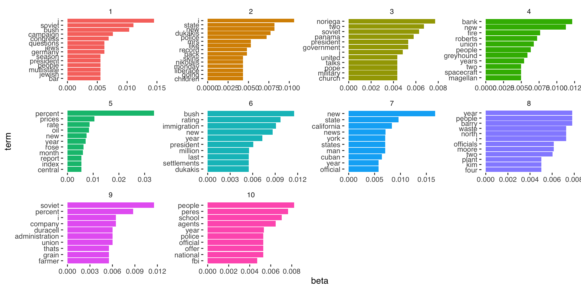
Plot
betaplot <- lda_beta %>%
  group_by(topic) %>%
  top_n(10, beta) %>%
  ungroup() %>%
  arrange(topic, -beta) %>%
  mutate(term = reorder_within(term, beta, topic)) %>%
  ggplot(aes(beta, term, fill = factor(topic))) +
  geom_col(show.legend = FALSE) +
  facet_wrap(~ topic, scales = "free", ncol = 4) +
  scale_y_reordered() +
  theme_tufte(base_family = "Helvetica")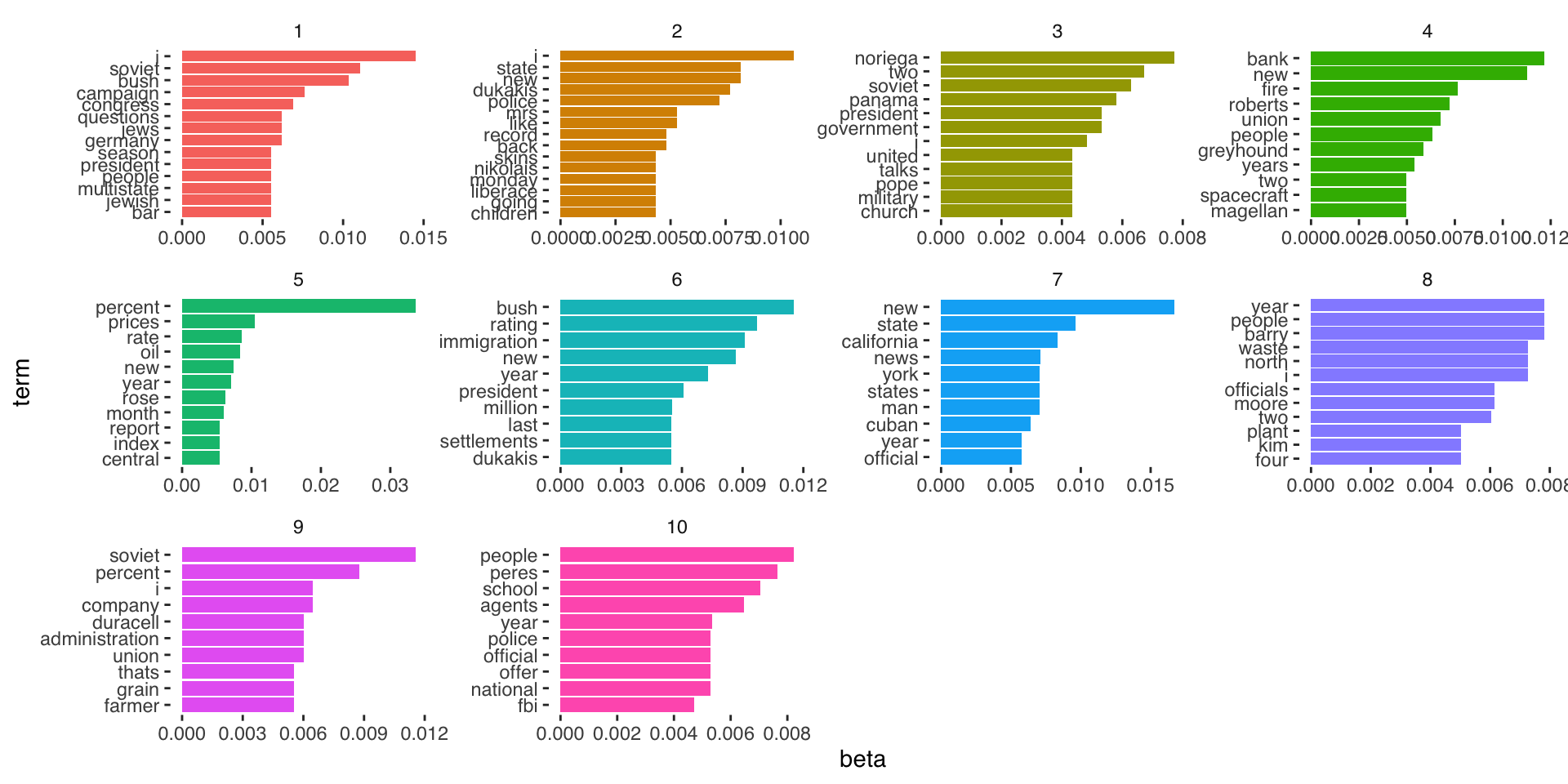
Word embedding
Data structure
Word pair matrix with PMI (Pairwise mutual information)
where PMI = log(P(x,y)/P(x)P(y))
and P(x,y) is the probability of word x appearing within a six-word window of word y
and P(x) is the probability of word x appearing in the whole corpus
and P(y) is the probability of word y appearing in the whole corpus
Data structure
6 x 6 sparse Matrix of class "dgCMatrix"
               the          to          and          of      https           a
the    0.653259169 -0.01948121 -0.006446459  0.27136395 -0.5246159 -0.32557524
to    -0.019481205  0.75498084 -0.065170433 -0.25694210 -0.5731182 -0.04595798
and   -0.006446459 -0.06517043  1.027782342 -0.03974904 -0.4915159 -0.05862969
of     0.271363948 -0.25694210 -0.039749043  1.02111517 -0.5045067  0.09829389
https -0.524615878 -0.57311817 -0.491515918 -0.50450674  0.5451841 -0.57956404
a     -0.325575239 -0.04595798 -0.058629689  0.09829389 -0.5795640  1.03048355
Data structure
Formal class 'dgCMatrix' [package "Matrix"] with 6 slots
  ..@ i       : int [1:350700] 0 1 2 3 4 5 6 7 8 9 ...
  ..@ p       : int [1:21173] 0 7819 14360 20175 25467 29910 34368 39207 43376 46401 ...
  ..@ Dim     : int [1:2] 21172 21172
  ..@ Dimnames:List of 2
  .. ..$ : chr [1:21172] "the" "to" "and" "of" ...
  .. ..$ : chr [1:21172] "the" "to" "and" "of" ...
  ..@ x       : num [1:350700] 0.65326 -0.01948 -0.00645 0.27136 -0.52462 ...
  ..@ factors : list()
Singular value decomposition
Singular value decomposition
Singular value decomposition
Singular value decomposition
              [,1]        [,2]        [,3]        [,4]        [,5]
the    0.007810973  0.07024009  0.06377615  0.03139044 -0.12362108
to     0.006889381 -0.03210269  0.10665925  0.03537632  0.10104552
and   -0.050498380  0.09131495  0.19658197 -0.08136253 -0.01605705
of    -0.015628371  0.16306386  0.13296127 -0.04087709 -0.23175976
https  0.301718525  0.07658843 -0.01720398  0.26219147  0.07930941
Word embeddings with GloVe
After we’ve generated our term co-ocurrence matrix…
DIM <- 300
ITERS <- 100
# ================================ set model parameters
# ================================
glove <- GlobalVectors$new(rank = DIM, x_max = 100, learning_rate = 0.05)

# ================================ fit model ================================
word_vectors_main <- glove$fit_transform(tcm, n_iter = ITERS, convergence_tol = 0.001,
    n_threads = RcppParallel::defaultNumThreads())