Introdução à Ciência de Dados no R
Aula 13 - Construindo Tabelas
Aula 13
Antonio Vinícius Barbosa
25-11-2023
![]()
Comunicação efetiva de dados
Comunicação efetiva de dados
- Na maioria dos relatórios, a comunicação dos resultados ocorre por meio de uma combinação de visualização de dados e tabelas
- No
R, há diversas maneiras de criar tabelas que comuniquem seus resultados com eficiência
Objetivo
Apresentar o
gt, um pacote flexível para a construção de tabelas
![]()
O pacote gt
- O pacote
gt(grammar oftables) permite a construção de tabelas através de ajustes nos seus elementos. - Basicamente, o pacote possibilita a transformação de um
data frameem tabelas elaboradas

Alguns exemplos
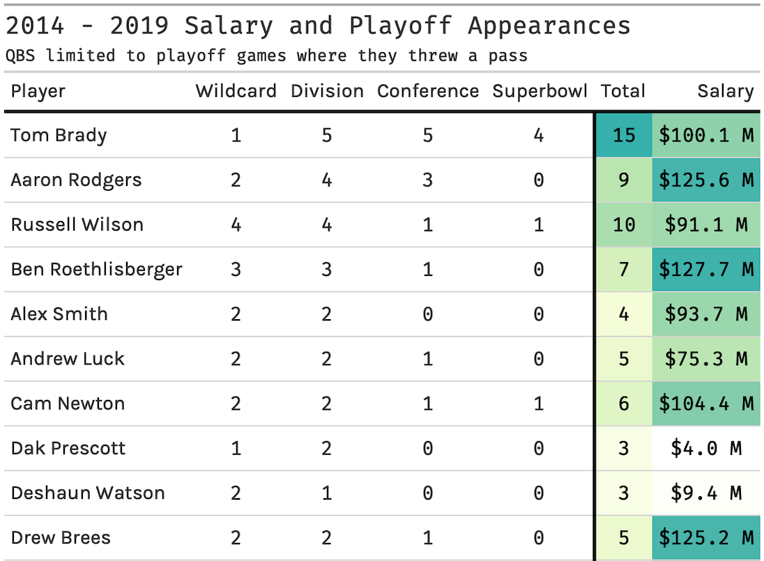
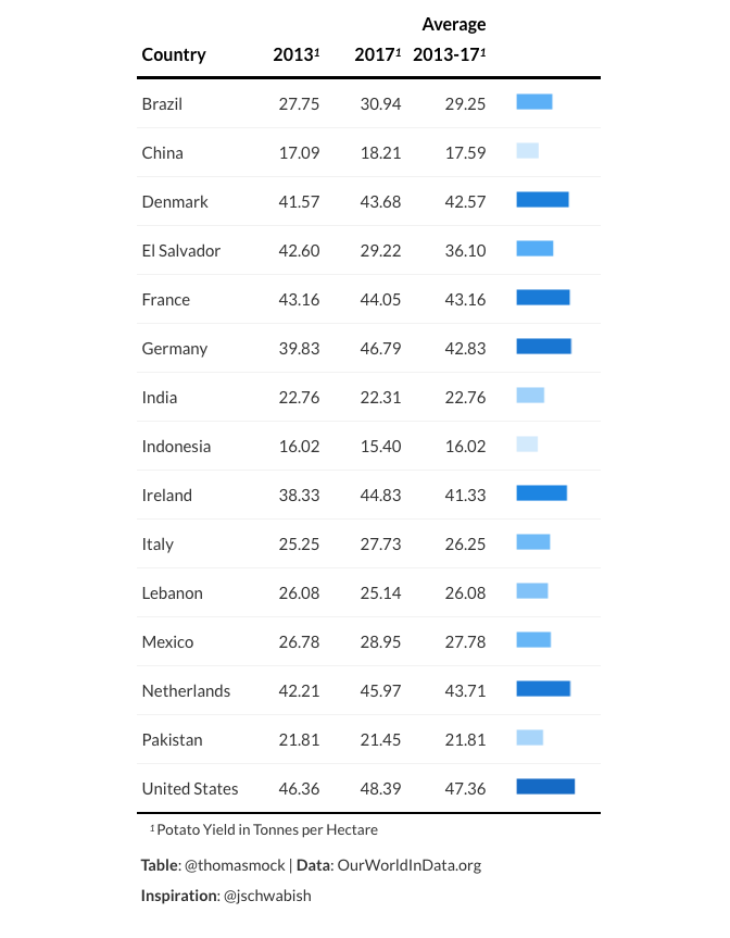
As partes de uma tabela
O gt estrutura a tabela em diferentes partes. Estas incluem table header, stub head, column labels, a table body e o table footer.

Instalação do gt
Dados
Para contruir as tabelas com gt, utilizaremos os dados de produção agrícola dos países
# Carregar url e ler dados
url <- 'https://raw.githubusercontent.com/rfordatascience/tidytuesday/master/data/2020/2020-09-01/key_crop_yields.csv'
prod_agricola <- readr::read_csv(url)
# Visualizar dados
prod_agricola
## # A tibble: 13,075 × 14
## Entity Code Year `Wheat (tonnes per hectare)` Rice (tonnes per hecta…¹
## <chr> <chr> <dbl> <dbl> <dbl>
## 1 Afghanistan AFG 1961 1.02 1.52
## 2 Afghanistan AFG 1962 0.974 1.52
## 3 Afghanistan AFG 1963 0.832 1.52
## 4 Afghanistan AFG 1964 0.951 1.73
## 5 Afghanistan AFG 1965 0.972 1.73
## 6 Afghanistan AFG 1966 0.867 1.52
## 7 Afghanistan AFG 1967 1.12 1.92
## 8 Afghanistan AFG 1968 1.16 1.95
## 9 Afghanistan AFG 1969 1.19 1.98
## 10 Afghanistan AFG 1970 0.956 1.81
## # ℹ 13,065 more rows
## # ℹ abbreviated name: ¹`Rice (tonnes per hectare)`
## # ℹ 9 more variables: `Maize (tonnes per hectare)` <dbl>,
## # `Soybeans (tonnes per hectare)` <dbl>,
## # `Potatoes (tonnes per hectare)` <dbl>, `Beans (tonnes per hectare)` <dbl>,
## # `Peas (tonnes per hectare)` <dbl>, `Cassava (tonnes per hectare)` <dbl>,
## # `Barley (tonnes per hectare)` <dbl>, …Dados
Manipulando os dados:
# Carregar pacote
library(tidyverse)

# Manipular dados
prod_agr_data <- prod_agricola |>
  janitor::clean_names() |>
  rename_with(
    ~str_remove(., "_tonnes_per_hectare")
    ) |>
  select(
    entity:beans, -code
    ) |>
  pivot_longer(
    cols = wheat:beans,
    names_to = "crop",
    values_to = "yield"
    ) |>
  rename(country = entity) |>
  filter(
    country %in% c("China", "United States", "Brazil"),
    year %in% 2016:2018,
    crop %in% c("maize", "soybeans")
    ) |>
  mutate(crop = case_when(
    crop == "maize" ~ "Milho",
    crop == "soybeans" ~ "Soja"
    )
  ) |>
  pivot_wider(
    names_from = year,
    values_from = yield
    )
Dados
Como resultado, obtemos:
gt básico
Para gerar uma tabela básica, fazemos:
Modificando o título
| Produção agrícola dos países | ||||
| Total da produção em toneladas por hectare | ||||
| country | crop | 2016 | 2017 | 2018 |
|---|---|---|---|---|
| Brazil | Milho | 4.2877 | 5.6183 | 5.1044 |
| Brazil | Soja | 2.9049 | 3.3785 | 3.3903 |
| China | Milho | 5.9667 | 6.1103 | 6.1042 |
| China | Soja | 1.8030 | 1.7862 | 1.7800 |
| United States | Milho | 11.7433 | 11.8754 | 11.8639 |
| United States | Soja | 3.4936 | 3.3133 | 3.4681 |
Adicionando a fonte dos dados
| Produção agrícola dos países | ||||
| Total da produção em toneladas por hectare | ||||
| country | crop | 2016 | 2017 | 2018 |
|---|---|---|---|---|
| Brazil | Milho | 4.2877 | 5.6183 | 5.1044 |
| Brazil | Soja | 2.9049 | 3.3785 | 3.3903 |
| China | Milho | 5.9667 | 6.1103 | 6.1042 |
| China | Soja | 1.8030 | 1.7862 | 1.7800 |
| United States | Milho | 11.7433 | 11.8754 | 11.8639 |
| United States | Soja | 3.4936 | 3.3133 | 3.4681 |
| Fonte: U.S. Department of Agriculture | ||||
Modificando o nome das colunas
| Produção agrícola dos países | ||||
| Total da produção em toneladas por hectare | ||||
| País | Produto | 2016 | 2017 | 2018 |
|---|---|---|---|---|
| Brazil | Milho | 4.2877 | 5.6183 | 5.1044 |
| Brazil | Soja | 2.9049 | 3.3785 | 3.3903 |
| China | Milho | 5.9667 | 6.1103 | 6.1042 |
| China | Soja | 1.8030 | 1.7862 | 1.7800 |
| United States | Milho | 11.7433 | 11.8754 | 11.8639 |
| United States | Soja | 3.4936 | 3.3133 | 3.4681 |
| Fonte: U.S. Department of Agriculture | ||||
Apresentando por grupos
| Produção agrícola dos países | |||
| Total de produção em toneladas por hectare | |||
| 2016 | 2017 | 2018 | |
|---|---|---|---|
| Brazil | |||
| Milho | 4.2877 | 5.6183 | 5.1044 |
| Soja | 2.9049 | 3.3785 | 3.3903 |
| China | |||
| Milho | 5.9667 | 6.1103 | 6.1042 |
| Soja | 1.8030 | 1.7862 | 1.7800 |
| United States | |||
| Milho | 11.7433 | 11.8754 | 11.8639 |
| Soja | 3.4936 | 3.3133 | 3.4681 |
| Fonte: U.S. Department of Agriculture | |||
Agrupando colunas
prod_agr_data |>
  group_by(country) |>
  gt(rowname_col = "crop") |>
  tab_header(
    title = md("**Produção agrícola dos países**"),
    subtitle = md("Total de produção em toneladas por hectare")) |>
tab_source_note(md("Fonte: [U.S. Department of Agriculture](https://www.usda.gov/)")) |>
tab_spanner(
label = "Ano",
columns = `2016`:`2018`
)| Produção agrícola dos países | |||
| Total de produção em toneladas por hectare | |||
| Ano | |||
|---|---|---|---|
| 2016 | 2017 | 2018 | |
| Brazil | |||
| Milho | 4.2877 | 5.6183 | 5.1044 |
| Soja | 2.9049 | 3.3785 | 3.3903 |
| China | |||
| Milho | 5.9667 | 6.1103 | 6.1042 |
| Soja | 1.8030 | 1.7862 | 1.7800 |
| United States | |||
| Milho | 11.7433 | 11.8754 | 11.8639 |
| Soja | 3.4936 | 3.3133 | 3.4681 |
| Fonte: U.S. Department of Agriculture | |||
Adicionando footnotes
prod_agr_data |>
  group_by(country) |>
  gt(rowname_col = "crop") |>
  tab_header(
    title = md("**Produção agrícola dos países**"),
    subtitle = md("Total de produção em toneladas por hectare")) |>
  tab_source_note(md("Fonte: [U.S. Department of Agriculture](https://www.usda.gov/)")) |>
  tab_spanner(
    label = "Ano",
    columns = `2016`:`2018`
) |>
tab_footnote(
footnote = "Quantidades baseadas em relatórios oficiais.",
locations = cells_title(groups = "subtitle")
) |>
tab_footnote(
footnote = "Dados projetados",
locations = cells_row_groups(groups = c("China"))
)| Produção agrícola dos países | |||
| Total de produção em toneladas por hectare1 | |||
| Ano | |||
|---|---|---|---|
| 2016 | 2017 | 2018 | |
| Brazil | |||
| Milho | 4.2877 | 5.6183 | 5.1044 |
| Soja | 2.9049 | 3.3785 | 3.3903 |
| China2 | |||
| Milho | 5.9667 | 6.1103 | 6.1042 |
| Soja | 1.8030 | 1.7862 | 1.7800 |
| United States | |||
| Milho | 11.7433 | 11.8754 | 11.8639 |
| Soja | 3.4936 | 3.3133 | 3.4681 |
| Fonte: U.S. Department of Agriculture | |||
| 1 Quantidades baseadas em relatórios oficiais. | |||
| 2 Dados projetados | |||
Formatando elementos das células
prod_agr_data |>
  group_by(country) |>
  gt(rowname_col = "crop") |>
  tab_header(
    title = md("**Produção agrícola dos países**"),
    subtitle = md("Total de produção em toneladas por hectare")) |>
  tab_source_note(md("Fonte: [U.S. Department of Agriculture](https://www.usda.gov/)")) |>
  tab_spanner(
    label = "Ano",
    columns = `2016`:`2018`
  ) |>
   tab_footnote(
    footnote = "Quantidades baseadas em relatórios oficiais.",
    locations = cells_title(groups = "subtitle")
  ) |>
fmt_number(decimals = 2)| Produção agrícola dos países | |||
| Total de produção em toneladas por hectare1 | |||
| Ano | |||
|---|---|---|---|
| 2016 | 2017 | 2018 | |
| Brazil | |||
| Milho | 4.29 | 5.62 | 5.10 |
| Soja | 2.90 | 3.38 | 3.39 |
| China | |||
| Milho | 5.97 | 6.11 | 6.10 |
| Soja | 1.80 | 1.79 | 1.78 |
| United States | |||
| Milho | 11.74 | 11.88 | 11.86 |
| Soja | 3.49 | 3.31 | 3.47 |
| Fonte: U.S. Department of Agriculture | |||
| 1 Quantidades baseadas em relatórios oficiais. | |||
Ajustando a aparência
prod_agr_data |>
  group_by(country) |>
  gt(rowname_col = "crop") |>
  tab_header(
    title = md("**Produção agrícola dos países**"),
    subtitle = md("Total de produção em toneladas por hectare")) |>
  tab_source_note(md("Fonte: [U.S. Department of Agriculture](https://www.usda.gov/)")) |>
  tab_spanner(
    label = "Ano",
    columns = `2016`:`2018`
  ) |>
   tab_footnote(
    footnote = "Quantidades baseadas em relatórios oficiais.",
    locations = cells_title(groups = "subtitle")
  ) |>
  fmt_number(decimals = 2) |>
  tab_options(
    heading.subtitle.font.size = 18,
    heading.background.color = "#C1EEFF",
    footnotes.font.size = 18,
    source_notes.font.size = 18,
    heading.align = "left",
    table.border.top.color = "black",
    table.border.bottom.color = "black",
    column_labels.border.bottom.color = "black"
)| Produção agrícola dos países | |||
| Total de produção em toneladas por hectare1 | |||
| Ano | |||
|---|---|---|---|
| 2016 | 2017 | 2018 | |
| Brazil | |||
| Milho | 4.29 | 5.62 | 5.10 |
| Soja | 2.90 | 3.38 | 3.39 |
| China | |||
| Milho | 5.97 | 6.11 | 6.10 |
| Soja | 1.80 | 1.79 | 1.78 |
| United States | |||
| Milho | 11.74 | 11.88 | 11.86 |
| Soja | 3.49 | 3.31 | 3.47 |
| Fonte: U.S. Department of Agriculture | |||
| 1 Quantidades baseadas em relatórios oficiais. | |||
Alterando a fonte
prod_agr_data |>
  group_by(country) |>
  gt(rowname_col = "crop") |>
  tab_header(
    title = md("**Produção agrícola dos países**"),
    subtitle = md("Total de produção em toneladas por hectare")) |>
  tab_source_note(md("Fonte: [U.S. Department of Agriculture](https://www.usda.gov/)")) |>
  tab_spanner(
    label = "Ano",
    columns = `2016`:`2018`
  ) |>
   tab_footnote(
    footnote = "Quantidades baseadas em relatórios oficiais.",
    locations = cells_title(groups = "subtitle")
  ) |>
  tab_options(
    heading.subtitle.font.size = 18,
    heading.background.color = "#C1EEFF",
    footnotes.font.size = 18,
    source_notes.font.size = 18,
    heading.align = "left",
    table.border.top.color = "black",
    table.border.bottom.color = "black",
    column_labels.border.bottom.color = "black",
    table.font.size = px(30),
  ) |>
  fmt_number(decimals = 2) |>
   opt_table_font(
    font = list(
      google_font(name = "Abel")
    )
)| Produção agrícola dos países | |||
| Total de produção em toneladas por hectare1 | |||
| Ano | |||
|---|---|---|---|
| 2016 | 2017 | 2018 | |
| Brazil | |||
| Milho | 4.29 | 5.62 | 5.10 |
| Soja | 2.90 | 3.38 | 3.39 |
| China | |||
| Milho | 5.97 | 6.11 | 6.10 |
| Soja | 1.80 | 1.79 | 1.78 |
| United States | |||
| Milho | 11.74 | 11.88 | 11.86 |
| Soja | 3.49 | 3.31 | 3.47 |
| Fonte: U.S. Department of Agriculture | |||
| 1 Quantidades baseadas em relatórios oficiais. | |||
Alterando as cores das células
prod_agr_data |>
  group_by(country) |>
  gt(rowname_col = "crop") |>
  tab_header(
    title = md("**Produção agrícola dos países**"),
    subtitle = md("Total de produção em toneladas por hectare")) |>
  tab_source_note(md("Fonte: [U.S. Department of Agriculture](https://www.usda.gov/)")) |>
  tab_spanner(
    label = "Ano",
    columns = `2016`:`2018`
  ) |>
   tab_footnote(
    footnote = "Quantidades baseadas em relatórios oficiais.",
    locations = cells_title(groups = "subtitle")
  ) |>
  tab_options(
    heading.subtitle.font.size = 18,
    heading.background.color = "#C1EEFF",
    footnotes.font.size = 18,
    source_notes.font.size = 18,
    heading.align = "left",
    table.border.top.color = "black",
    table.border.bottom.color = "black",
    column_labels.border.bottom.color = "black",
    table.font.size = px(30),
  ) |>
  fmt_number(decimals = 2) |>
   opt_table_font(
    font = list(
      google_font(name = "Abel")
    )
  ) |>
  data_color(
    method = "numeric",
    palette = c("#A0D2DB", "#424874")
)| Produção agrícola dos países | |||
| Total de produção em toneladas por hectare1 | |||
| Ano | |||
|---|---|---|---|
| 2016 | 2017 | 2018 | |
| Brazil | |||
| Milho | 4.29 | 5.62 | 5.10 |
| Soja | 2.90 | 3.38 | 3.39 |
| China | |||
| Milho | 5.97 | 6.11 | 6.10 |
| Soja | 1.80 | 1.79 | 1.78 |
| United States | |||
| Milho | 11.74 | 11.88 | 11.86 |
| Soja | 3.49 | 3.31 | 3.47 |
| Fonte: U.S. Department of Agriculture | |||
| 1 Quantidades baseadas em relatórios oficiais. | |||
Quizz #1
Agora é a sua vez de gerar uma tabela com gt
- Utilizar a base disponível em
dados::dados_gapminder - Filtrar para os anos de 1952, 1977 e 2007
- Apresentar uma tabela agrupada por continente e mostrar a evolução das variáveis. Os anos são apresentados nas linhas.
- Adicionar um título e um subtítulo para o tabela, além da fonte dos dados.
- Através da função
fmt_currency, adicionar o cifrão ($) para a variável do pib per capita. Além disso, utilizar apenas 2 casas decimais para essa variável. - Apresentar as informações por grupos de continentes.
- Mudar o nome das variáveis.
- Alterar a fonte e demais aspectos visuais.
20:00
Referências
Materias de referência para o gt
Outros pacotes para construção de tabelas
ICDR