Report - Niklaus Houska & Alessia Paccagnella

Alessia

1. Image Textures

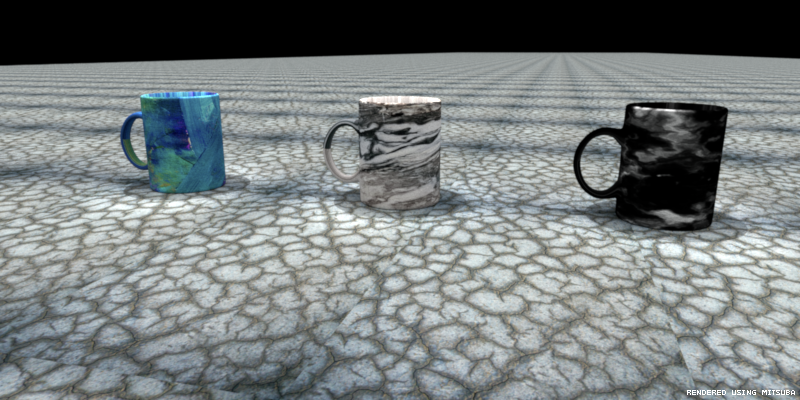
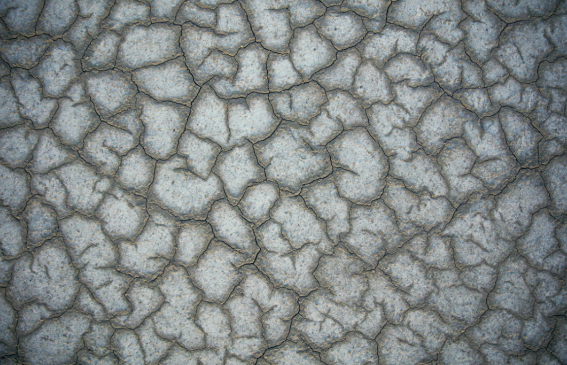
I implemented the images as texture feature using PNG images. For this, I had to use the lodepng library. this link helped me understanding how to access the pixel value. I basically have a vector made of "RGBA RGBA RGBA..." values for each pixel, and uv coordinates. So the main problem was finding the index of the pixel in that vector.
The texture is scaled by a scale parameter and applied over the shape I choose. I scaled the texture3 used for the ground.
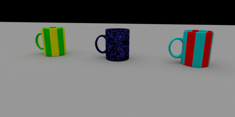
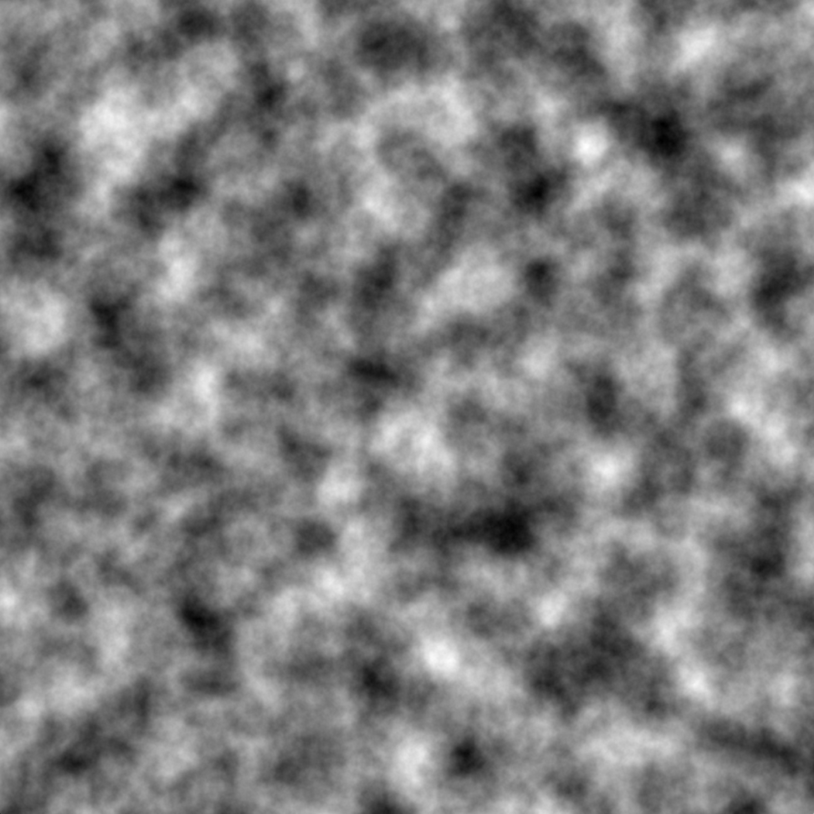
I also try to scale the perlin noise, on the left image that can be seen here.
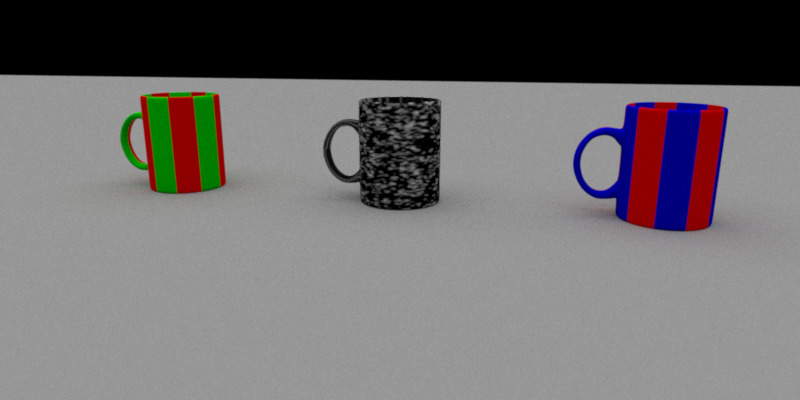
The first one is obtained scaling the perlin noise (texture 4) by 0.50, 0.50. The second one is obtained without scaling the perlin noise texture.


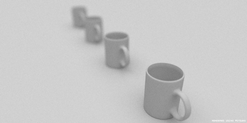
This is the Mitsuba version of the rendering, with the perlin texture NOT scaled: they apply the textures the same way, but the colors are a bit different, probably because of the library I use to extract pngs.

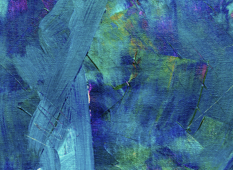
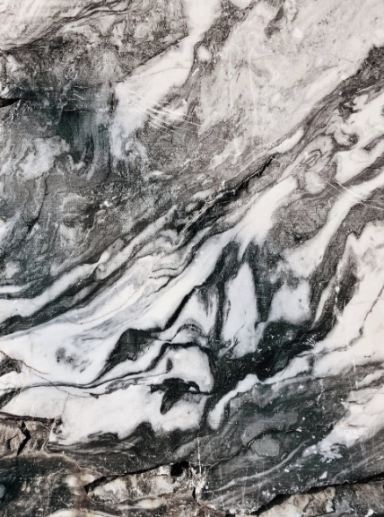
These are the four textures that I used:

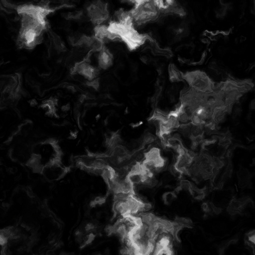
2. Procedural Textures

For this feature, I first tried to generate a procedural texture made of colored stripes. I enabled the possibility of choosing the scaling factor, the two colors and the delta factor. The implementation was quite straightforward. The code can be found in the class proceduraltexture.cpp.
Then I tried to implement the perlin noise. I spent a lot of time on this, because I was using some noise function that were not optimal for the aim of generating the perlin one. At the end, I followed this reference to implement it.
The noise function used in Perlin noise is a seeded random number generator. It returns the same value every time it is called with the same values for input. Then, I smoothed out the values that this noise function returned by using a cosine interpolation function, which worked better than the linear one because returned a much smother curve.
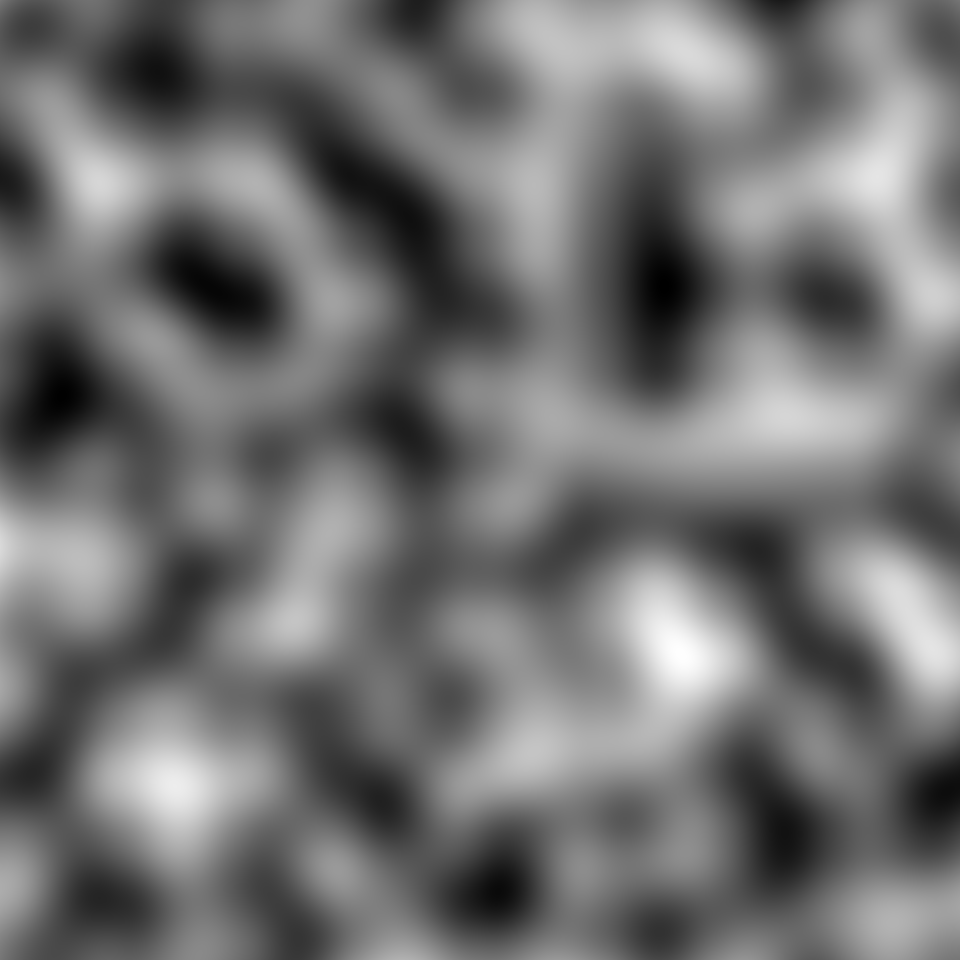
I used some variables like octaves, lacunarity and frequency to modify the noisy function created. An octave is each successive noise function that is added. I decided to use 9 octaves. Each noise function added had twice the frequency of the previous one. I did some trials with a bigger number but after a certain number one had a too high a frequency to be displayable.

The centered cup displayes the procedural perlin noise in two different colors.


Here examples of perlin noise taken from here , here and here can be seen.

3. Advanced Camera Model: Depth of field, Lens distortion, Chromatic Aberration

The code for these features can be found inside perspective.cpp.

3.1. Depth of field

To implement the depth of field, I added two extra parameters to the camera. One is the size of the lens aperture, and the other is the focal distance. I pass them throug the xml file of the scene.
I modified the file perspective.cpp: if depth of field is activated for the scene, the ray’s origin and direction are modified so that depth of field is simulated. I calculated the intersection of the ray through the lens center with the plane of focus, and then initialized the ray: its origin is set to the sampled point on the lens, its direction is initialized so that the ray passes through the point on the plane of focus.
ray.mint and ray.maxt remains the same of the previously provided code.
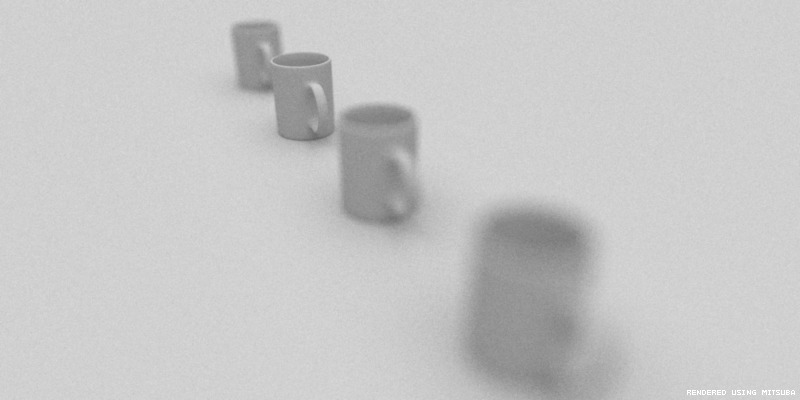
Following, different trials can be seen.

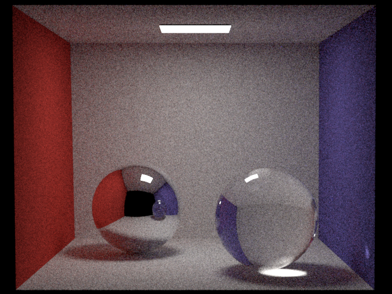
Focal Length = 8, radius = 0.2

The first image represents a focal length of 8, and a radius of 0.2. We can see that a small radius and a small focal length lead to focusing on the closer cup.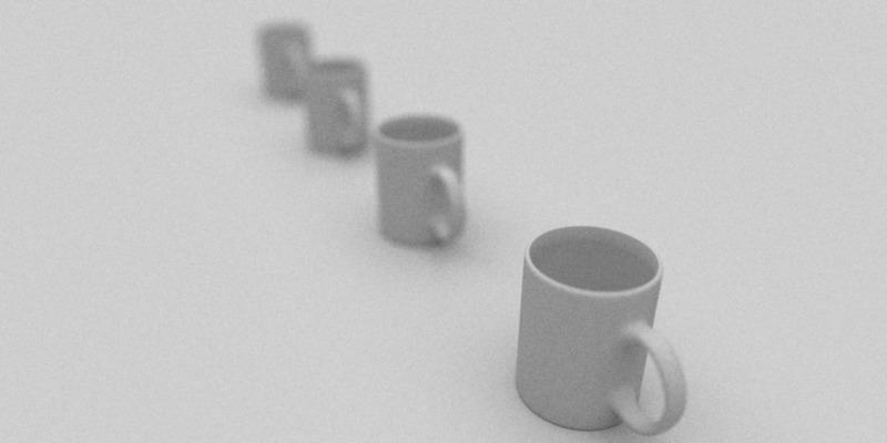

Focal Length = 15, radius = 0.2

The second represents a focal length of 15 and a radius of 0.2. Due to a higher focal length, we see that the closest cups are not focused anymore, differently from the ones more distant.

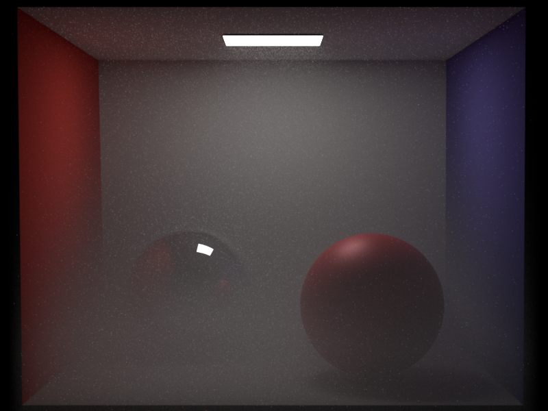
Focal Length = 15, radius = 0.5

Finally, the last one represents a focal length of 15, and a radius of 0.5. Here, by putting a longer radius we see that a smaller area is focused.

3.2. Lens Distortion

This feature extends the perspective camera with the effect of radial distortion. I added three extra parameters, which are change1 and change2, the second and fourth-order terms in a polynomial function that models the barrel distortion, and the boolean m_distortion, which indicates if the distortion is activated or not. After I calculate the distortion, with the function calculateDistortion(), I multiply the x and y coordinates of the position on the near plane for this factor. I followed mitsuba for calculating the distortion.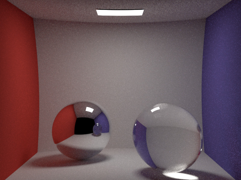

3.3. Chromatic aberration:

Chromatic aberration effect was quite tricky. If the effect is activated, in the render.cpp file the function sampleRay() of my camera class is called 3 times, one for each color channel. At the end, the value considered is the sum of the three values obtained.
In the sampleRay() method, I select the weight of the aberration for that color channel based on the index that it is passed to it. The weights are chosen directly from the xml file. Then, the position sample is normalized to be zero centered. After that, the point on plane of focus is shifted in the x and y direction.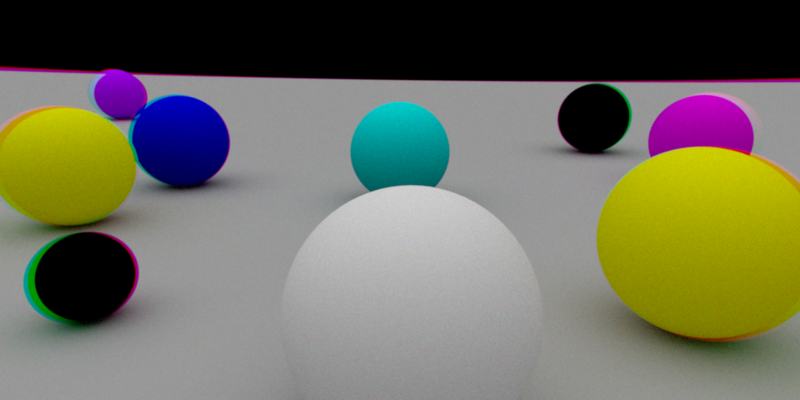

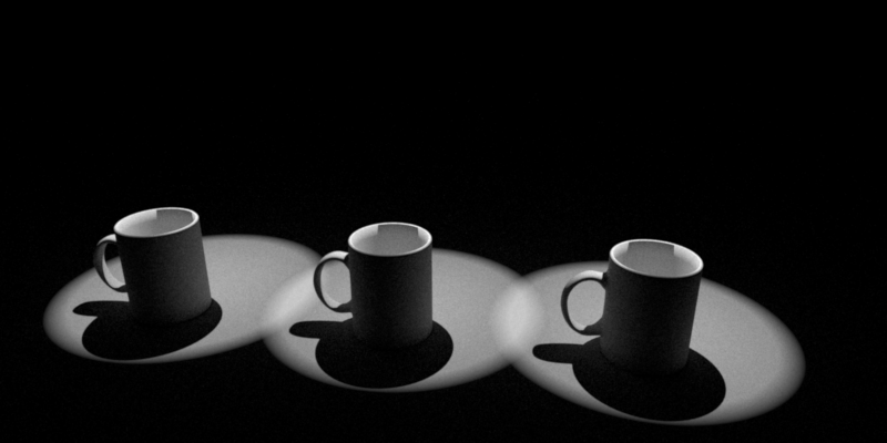
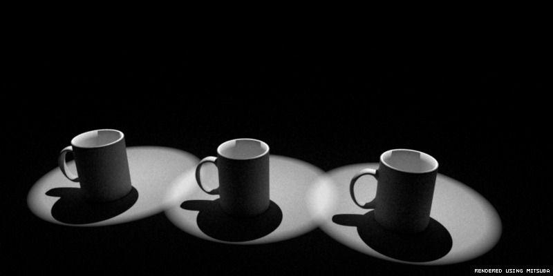
4. Spotlight

For this feature, I implemented a spotlight based on the implementation in the book "Physically based rendering".
Spotlights are a variation of point lights: they emit light in a cone of directions from their position instead of shining in all the directions. The functions are very similar to the ones written for pointlight.cpp. For example the sample() method is almost identical to the pointlight's one, except for the fact that it calls the cutOff() method, which computes the distribution of light accounting for the spotlight cone. For this function, due to the fact that I am comparing the results with Mitsuba, I changed the return value of the function cutOff according to Mitsuba implementation.
The parameters I input to the spotlight are cosFalloffStart,cosTotalWidth and the direction I want the spotlight to point to.
The code can be found inside spotlight.cpp.

Here we can see the validation:

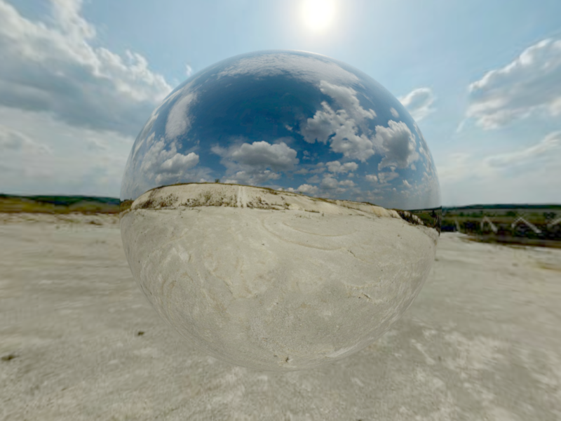
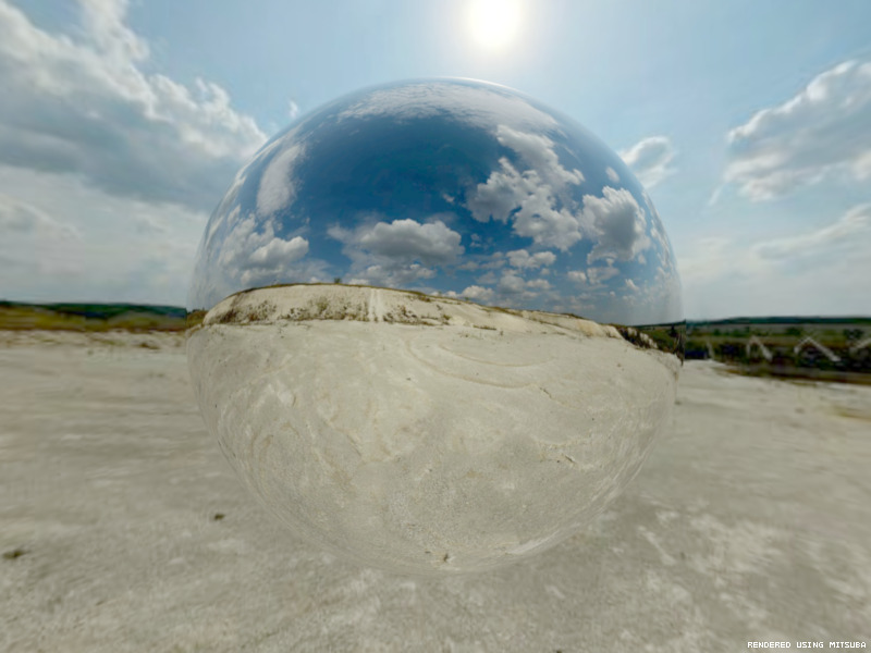
5. Environmental Map Emitter

The environmental map emitter was one of the features that took more time to be implemented. This paper helped me a lot. I followed the pseudo code given in that paper to implement the functions precomputer1D() and sample1D().
In the paper, importance sampling an envmap depends on the intensity distribution of the light texture. The made assumption is that that illumination in images is represented using latitude-longitude parameters. In fact the sample() method samples points and converts them to spherical coordinates for sampling the sphere.
I updated my path_mis class making sure that it worked properly with my EnvMap implementation.
As a first result, I obtained a very pixelated background. Then I changed the order of inputs in the bilinear interpolation and it looked much better.
The code can be found inside envmap.cpp.

I also added a strenght parameter to envmap, which multiplies what the eval() method returns in order to obtain a brighter result.

I downloaded the texture from here . In my scene I put a conductor sphere of radius 4. The envmap sphere is modeled by a sphere of radius of 30.

6. NL means denoising:

To complete this task, I implemented a matlab function following the pseudocode given in the slides from the lectures. I added the optimization for the fast implementation, that updates datvar as the maximum between datvar and the convolution of datvar and box2. To initialize the box filter, I used the function fspecial of Matlab, and used the size of 2*f+1 for it, where each entry gets assigned 1/num_entries.
The inputs of the function are f, r, k, I used the values given in the slides from lecture (3,10,0.45).
In order to use the function with exr files, I had to install the tool openexr for matlab.
In order to obtain the variance in exr format, I had to modify the code from render.cpp. I used the same structures (ImageBlock and BitMap) used in the provided code to save the original rendered image in that class.
I applied the function to the cbox scene generated for path_mats function.
The code is inside the file Nldenoise.m, inside the folder Matlab.
Here the result:

7. Extra:

I implemented the conductor feature just to use it for one of the renderings, but I don't submit it for grading.

Niklaus

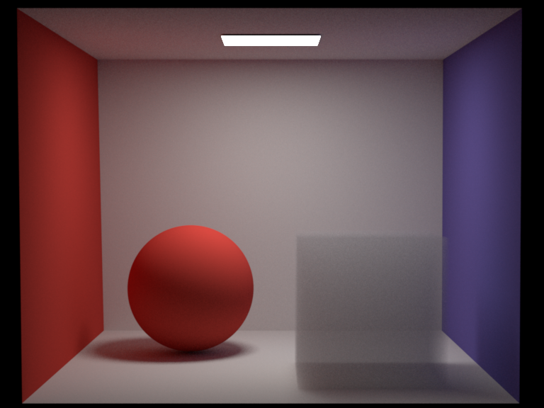
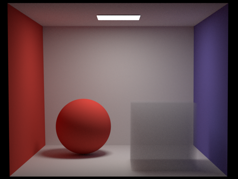
1. Heterogeneous Participating Media

Relevant classes
medium.h/.cpp
PhaseFunction.h/.cpp
vol_path.cpp

In following section the implementation of the heterogeneous medium and the volumetric path tracer (mis) are presented.

Medium

Our medium is described by the absorption and scattering coefficients sigma_a and sigma_s and a phase function. sigma_t the extinction coefficient and the color albedo can be derived from sigma_a and sigma_s . Each point in the medium has a density value determined by a function of choice. For simplicity the medium is bounded by a parameterized box, such that density evaluates to 0 outside the box.
We need two main functionalities from our medium class. We need to be able to sample an medium interaction given a ray and be able to determine the transmittance along a ray. To sample a medium interaction, we take a random step along the ray according to -log(1 - random) / sigma_t . Where random is a number between 0 and 1. If the normalized density at the observed spot is bigger than another random number, we report the medium interaction and return the interaction color albedo * density_at_location , else we continue. If the end of the ray is reached or the bounding box is exited, no medium interaction is made.
The transmittance is caluclated similarly. We step along the ray according to -log(1 - random) / sigma_t until we reach the end of the ray or leave the mediums bounding box. At each step we multiply the initial transmittance of 1 by 1 - density_at_location where the density is normalized to lie between 0 and 1.
For the density function I implemeted a simple exponential decay function a * exp(-b*h) .

sigma_a = 0.2 and sigma_s = 2 . Sample count 1024.

Volumetric Path Tracer

The path tracer is the core of the whole and took the most time to implement. As we are interested in a multiple importance sampler, I started by extending the MIS-path tracer already implemented in the exercises. Outline of the changed code:

t = (1,1,1), w_mats = 1
rayIntersect(...)
while (true)
  mediumColor = medium->sample_interaction(ray)
  if (medium interaction)

      pdf_mat, wo = sample_phaseFunction(ray)

      sample light and get pdf_ems
      if (shadowRay unoccluded)
          t *= mediumColor
          result += t * transmittance_to_light * pdf_mat * light_sample

      Russian Roulette

      ray = new Ray (origin=medium interaction, direction=wo)
      new w_mats weight if new intersection is emitter

  else if (not ray intersected)
      return result

  else
      -- Here comes surface interaction. Same as in path-mis except added transmission term to each light contribution
      -- and except that we dont return if the new ray does not intersect the scene
      -- to allow a further medium interaction

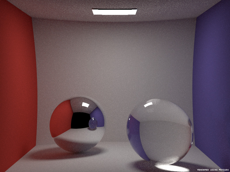
Validation

Here a comparison between the new integrator without a medium and the old mis path tracer. They are identical.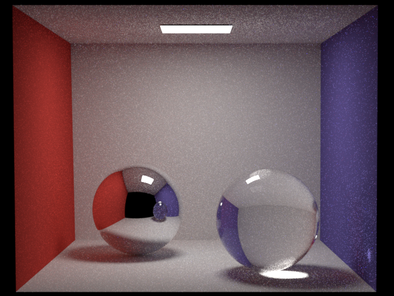

Next we show comparison of mitsuba with mine solution. The scenes geometry is not 100% identical due to conversion issues.
sigma_a = 1 and sigma_s = 2 . Sample count 256.

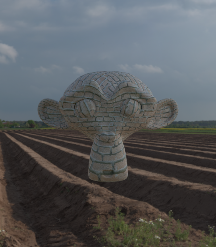
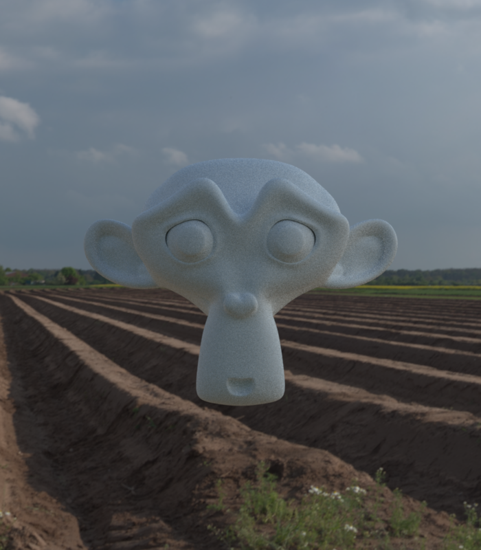
Bump Mapping

Relevant classes
normaltexture.cpp
vol_path.cpp
path_mis.cpp

Here I implemented a simple normal map texture. The color channels of the normal map are transformed into normal vector components according to 2 * c - 1 . The normal texture is added as a nested texture to any bsdf and the uv coordinate is used to look up the value. Furthermore, the texture can be scaled in the same way as the image texture.
The main integrators vol_path and path_mis where adapted to construct the new coordinate frame based on the looked up normal.
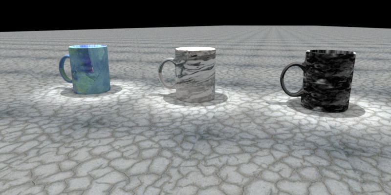
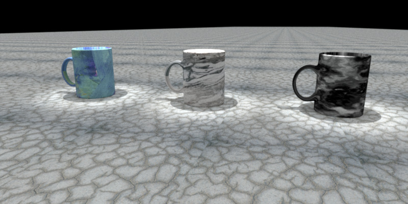
Below is a comparison of the normal maps effect. The images in the bottom row have a constant normal map evaluating to (0,0,1) everywhere.

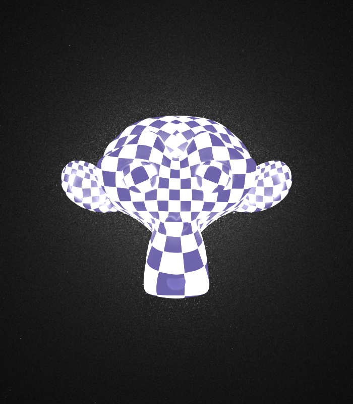
3. Textured Emitter

Relevant classes
arealight.cpp

To make textured emitters work, I added the functionality to add a texture to the area emitter. The area emitter is not anymore limited to a constant color but can use the uv coordinates to look up the radiance of a specified point. For this I added the possibility to pass uv coordinates within the EmitterQueryRecord and adapted the integrators to do so.
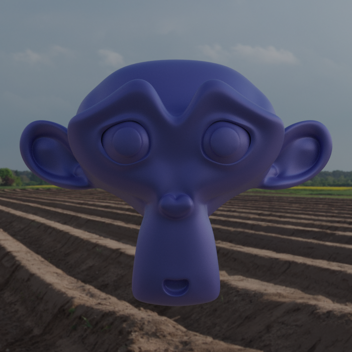
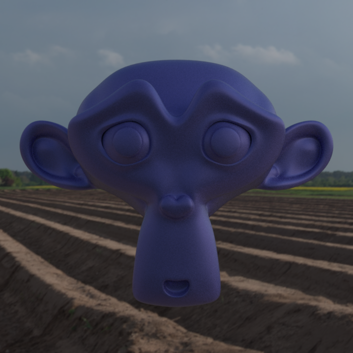
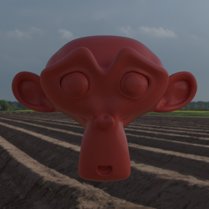
Below you see Suzanne (Blenders monkey) having a checkerboard textured area emitter as texture. Rendered using vol_path in light fog.

4. Disney BRDF

Relevant classes
disney.cpp
warp.cpp

BRDF evaluation

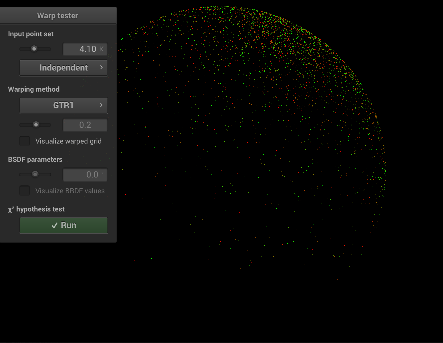
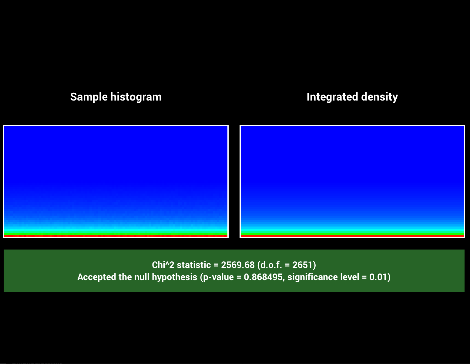
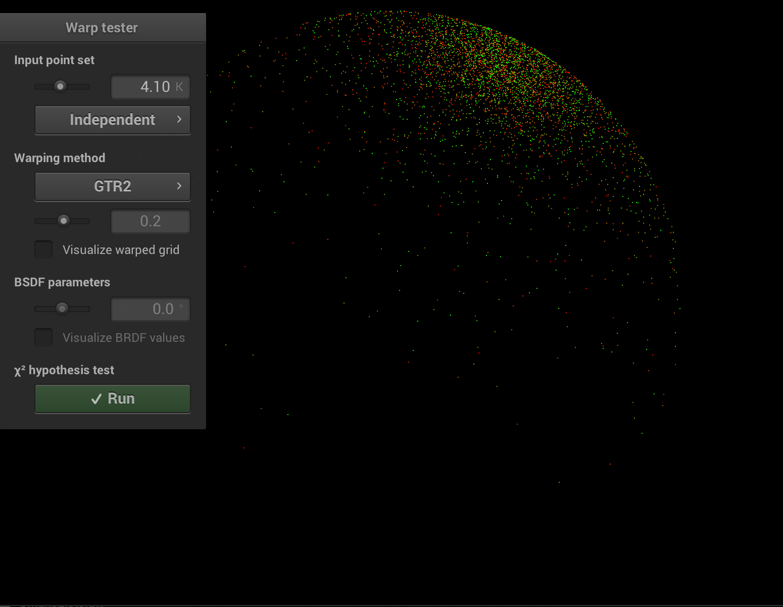
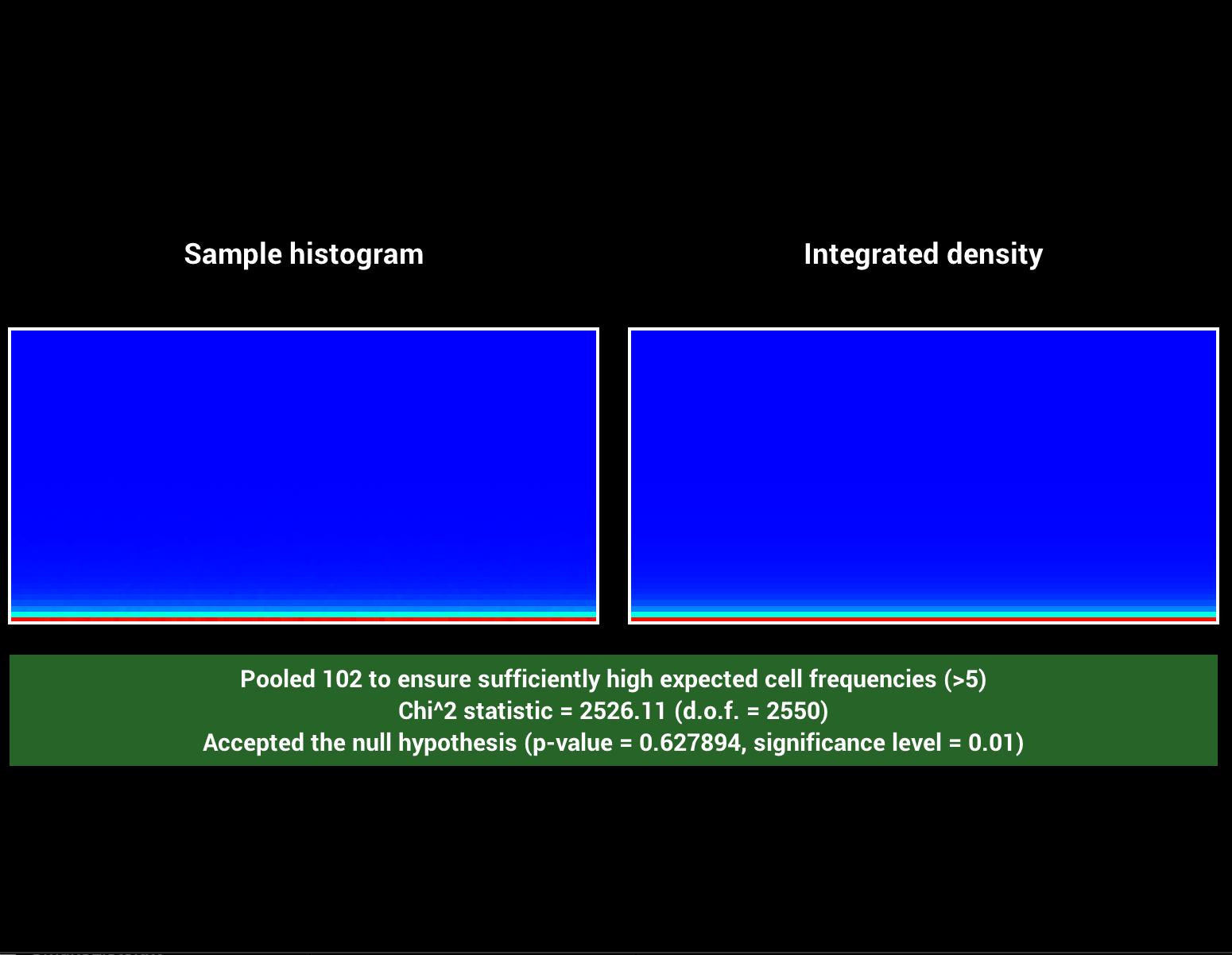
The evaluation of the brdf for a given pair of direction was implemented with help of this. I implemented the diffuse, roughness, specularity + tint, metallic and clearcoat + gloss parameters. Omitting subsurface scattering and anisotropic effects. There exist several small variants to the diffuse and specularity implementation, which I think comes due to artist preference. To describe the specular lobes we need two variants of the Generalized-Trowbridge-Reit distribution (or GTR), one for the specularity term (GTR2) and another one for the clearcoat term (GTR1). The SquareToGTR1/2 functions where added to the warp classes and verified using warptest as seen later in the report. Noteworthy is that we square the roughness parameter for the specularity evaluation, many materials show very low roughness values and the squaring makes it more natural to arrive to them. Clearcoat uses a hardcoded range of roughness adjustable through the clearcoat gloss parameter.

Below each image sequence varies one parameter while keeping the others constant.
Metallic (1, pink), Specular (2, blue), Specular Tint (3, yellow), Roughness (4, green), Clearcoat (5, red), Clearcoat Gloss (6, red)

0           0.1           0.3           0.5           0.7           0.9           1

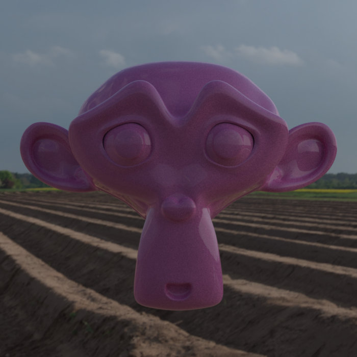
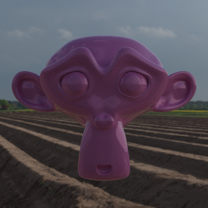
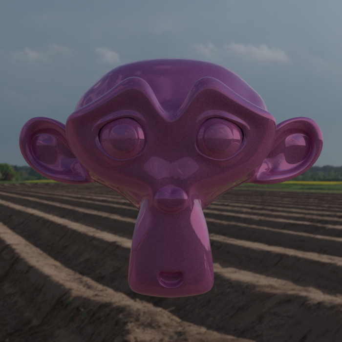
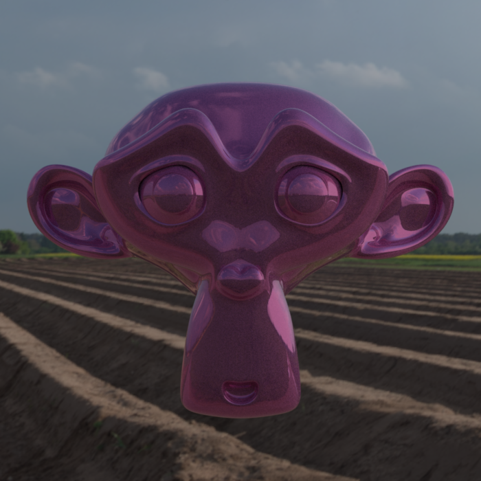
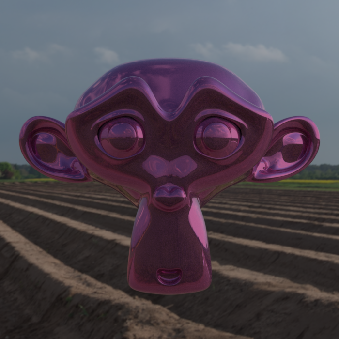
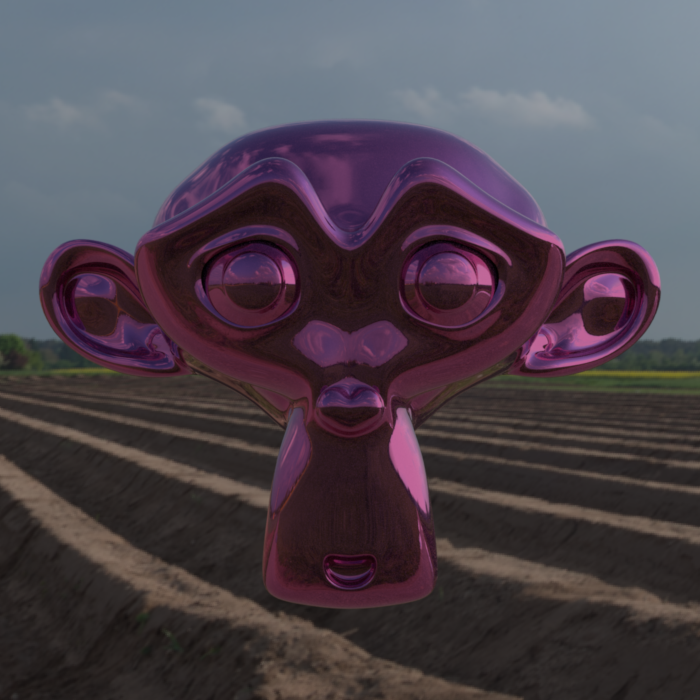
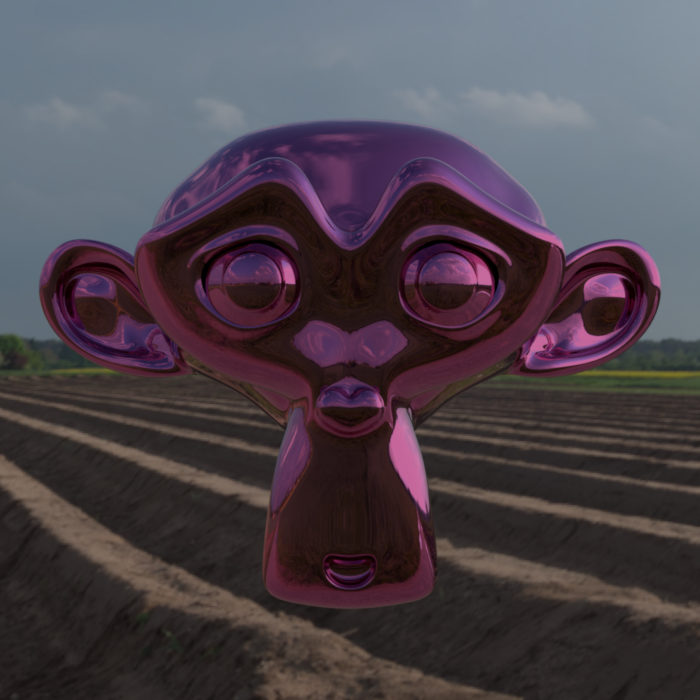
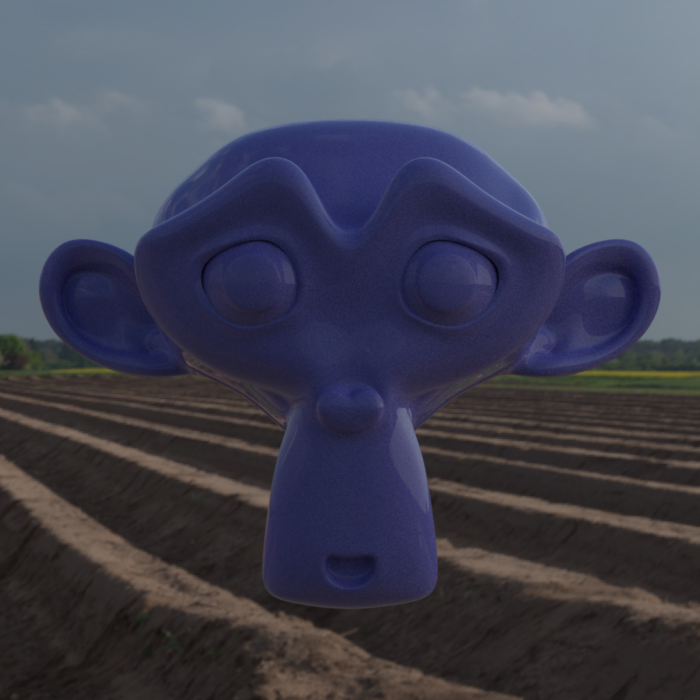
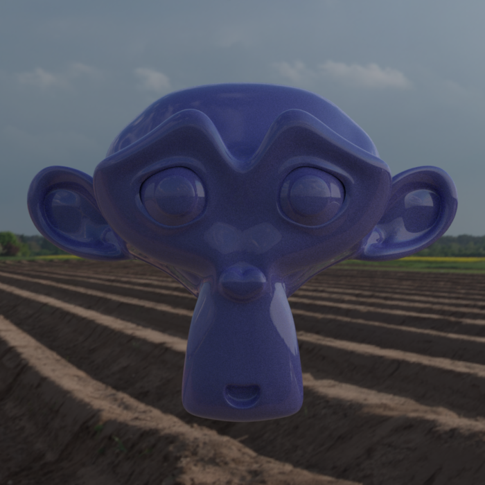
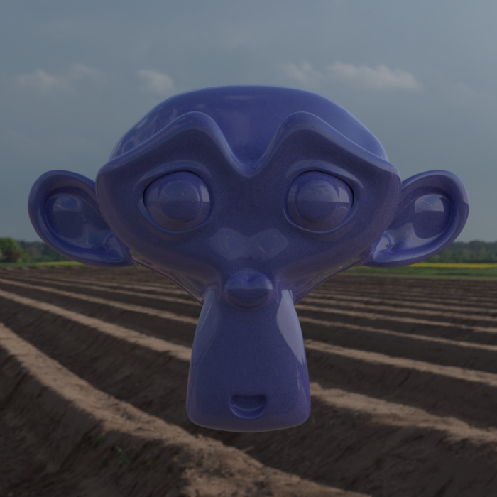
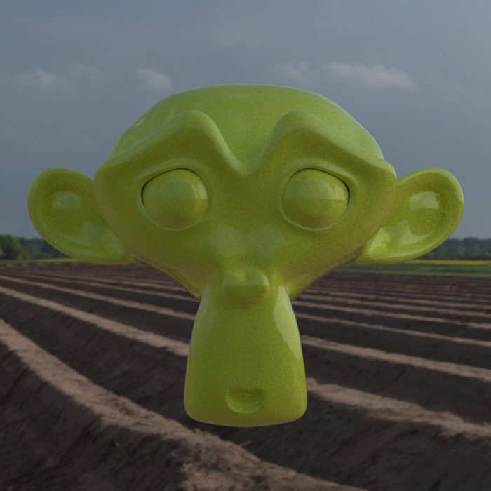
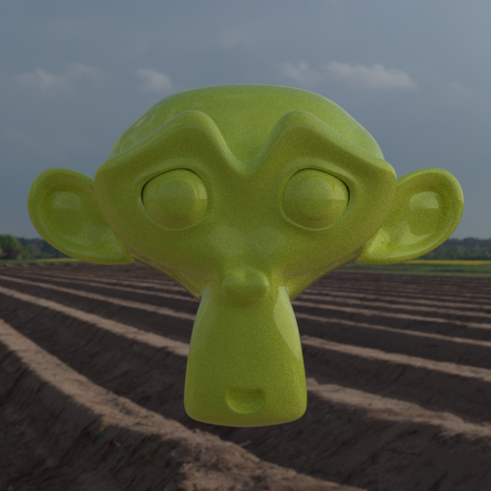
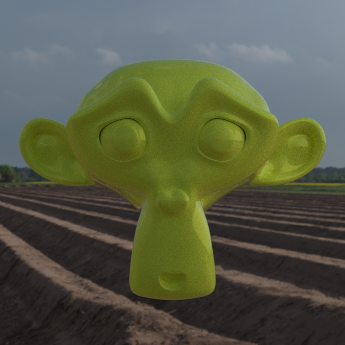
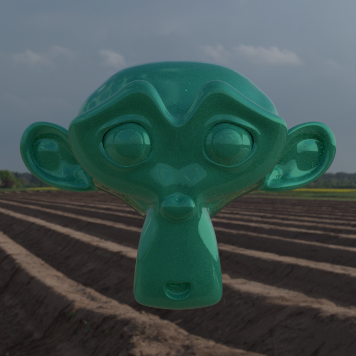
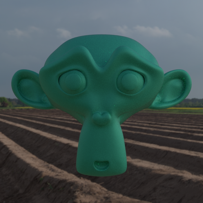
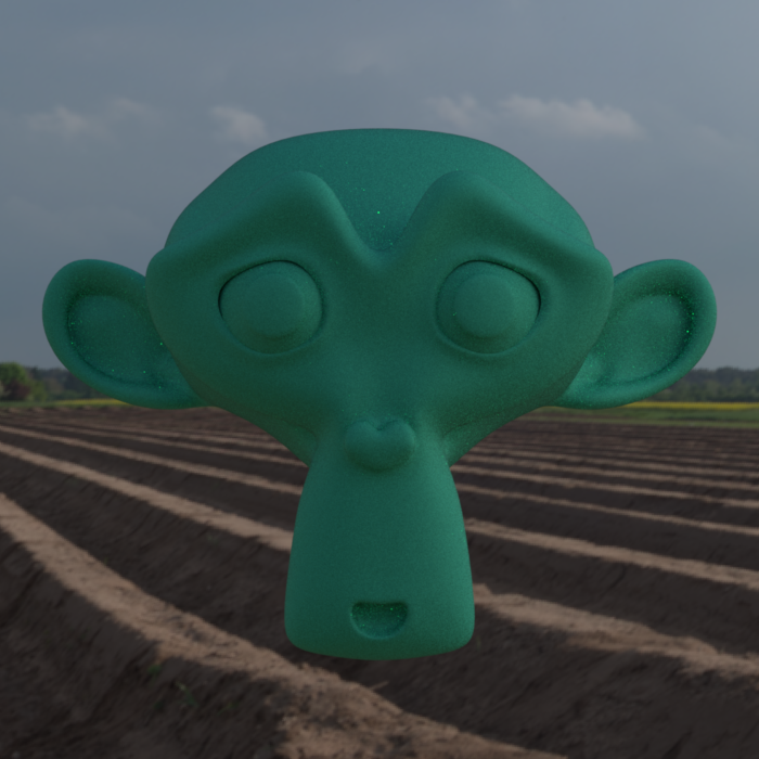
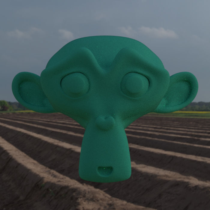
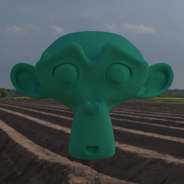
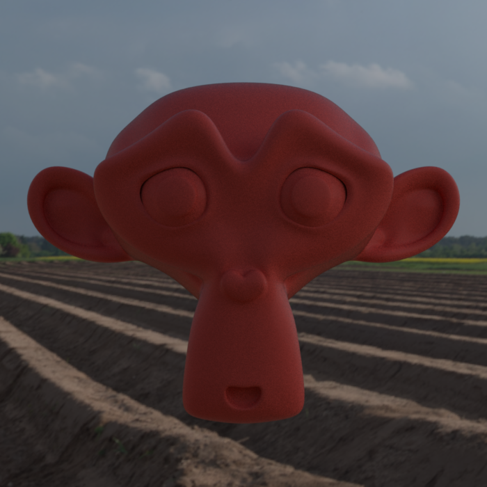
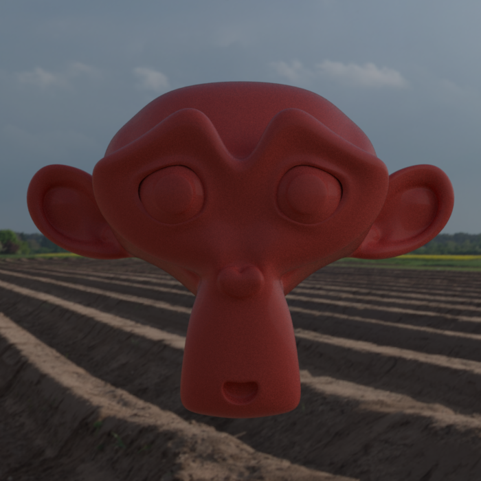
To compare the implementation with a reference, I took the Principled BSDF of blender