Introduction
Welcome to 318!
For this course we are going to integrate coding into our lectures.
This is the first of four tutorials that accompany the lectures.
These tutorials are focused on basic computational methods in macroeconomics.
In this first tutorial we will explore some basic programming topics.
The first tutorial is long, but not all the sections are needed to complete the exercises.
I will indicate which sections are optional.
Your interest in computational work will determine how much of this guide you read.
- Very interested -- Read the entire notebook (even if you don't understand everything)
- Somewhat interested -- Read through the notebook and scan through the
optionalsections- No interest -- Only read the slides (compulsory) so that you can complete the tutorials
My advice is to work on the notebook for 30 minutes at a time.
Try not to let the amount of information overwhelm you.
If you get stuck at some point just keep moving ahead, you can always come back.
I chose the Julia programming language because it is easy to learn and also very fast!
There are other excellent languages, such as Python, R and Matlab, which are useful for economists.
This notebook is meant to be used as a reference.
I am NOT expecting you to remember everything in the notebook!
While this is a reference, it only covers the very basic components of the language. Some other useful references that I used in constructing these notes are
You can ask me for more resources if you need it.
A good textbook that teaches both Julia and programming is Think Julia, which can be found here
Tutorial outline
In this course we hope to look at different themes in computational macroeconomics.
Most of modern macroeconomic research involves utilising computational methods, so it is worthwhile to get comfortable with some basic programming skills.
The return on this investment is quite high.
If you are interested in this type of work, feel free to contact me to talk about computational economics in Honours and Masters.
Here are some of the focus areas
- Fundamentals of programming (Lectures 1 - 3)
- Data, math and stats (Lectures 4 - 6)
- Optimisation and the consumer problem (Lectures 7 - 12)
- Solow model (Lectures 13 - 16)
Tutorial workflow
A problem set will be provided before each tutorial that contains two questions.
You must work on these questions before the tutorial.
During the live tutorial session I will be answering questions and then I will provide a third unseen question for you to work on.
There will be both normal pen and pencil exercises and computer based exercises.
For the best experience with this module it is strongly advised that students go through the tutorial material before the tutorials!
Running the notebooks
The current notes are put together in a Jupyter notebook.
There are several ways to view the notebooks. You can view the notebooks statically, which means that you will not be able to run the code.
If you want to do this then simply click on the HTML link on the GitHub page.
If you want to work interactively with notebooks then you need to install Anaconda and Julia.
Here is a link that explains the installation process.
It is preferred that you install the program on your computer.
However, if you are finding it difficult to get things working you may try the other options.
I will make a brief video on how to install Anaconda and link it to Julia.
Topics for the tutorial
Below are the broad topics for the tutorial
- Variables
- Data structures
- Control flow
- Functions
- Visualisation
- Type system and generic programming
Most of these topics are covered in introductory undergraduate computer science courses, so if you are a CS student then you can quickly skim for the Julia syntax.
If you are comfortable with a modern programming language like Python then everything here will feel somewhat familiar.
Your first code!
There are many great guides that provide an introduction to Julia and programming.
The QuantEcon website is an exceptional resource that can be used to teach yourself about computational economics.
We will be borrowing some of the material from their website in this section.
The main difference with these notes is that they are not nearly as comprehensive and are only meant as a starting point for your journey.
Before we start our discussion, let us try and run our first Julia program.
For those that have done programming before, this normally entails writing a piece of code that gives us the output Hello World!.
In Julia this is super easy to do.
println("Hello World!")
Congratulations you have run your first Julia code!
Introduction to packages
Julia has many useful packages. If we want to include a specific package then we can do the following,
import Pkg
Pkg.add("PackageName")
using PackageName
We show the process with the a few packages below.
NB: Make sure you run these lines, otherwise you will not be able to use the packages. You need to run these lines every time you start a new session.
import Pkg
Here are some of the packages that we are going to use in this tutorial. This will take a minute or two to install.
Pkg.add("DataFrames") # Package for working with data
Pkg.add("GLM") # Package for linear regression
Pkg.add("LinearAlgebra") # Package for linear algebra applications
Pkg.add("Plots") # Package for plotting
Pkg.add("TypeTree") # Package that shows type hierarchy in tree form
The using command lets the computer know that you are going to be using the following installed packages in your session. This is similar to import in Python or library() in R.
using Base: show_supertypes
using DataFrames
using GLM
using LinearAlgebra
using Plots
using TypeTree
We can now use basic functions from these packages. In the following section you will see how we use specific functions from the packages that we have installed.
Variables and types
After having successfully written your Hello World! code in Julia, a natural place to continue your journey is with variables.
A variable in a programming language is going to be some sort of symbol that we assign some value.
Let us use a concrete example to illustrate.
x = 2 # We assign the value of 2 to the variable x
In programming, variables are of a certain type, depending on the value or data assigned to the variable.
The type of the x variable is inferred automatically and we can check what this type is going to be by using the typeof() function.
typeof(x) # Command to find the type of the x variable
We see that the type of the variable is Int64.
What is an Int64?
This is an integer!
Integers are just the way that the computer records whole numbers.
Type Tree (optional)
This variable is of type Int64, which is actually part of the broader Integer type in Julia.
How do we know this? Well we need to look at the type tree.
A type tree gives us information about the different types and their relation to each other.
If we look at the type tree in the code below, we see that Int64 falls within the Integer class.
Int64 is a subtype of the broader Integer type, as can be seen below.
Note: If this type information seems strange to you right now, don't worry. We will repeatedly talk about types throughout the tutorial. You can always come back and read this section again later to make sure you understand.
print(join(tt(Integer), "")) # Print the subtypes of the `Integer` type.
We can also see the super types of the Int64 type.
All the types "above" Int64 in the type hierarchy are known as abstract types, while Int64 is a concrete type.
We will talk about abstract and concrete types again in the last section.
show_supertypes(Int64) # Show the super types of `Int64`
Variables and types contd.
We see from above that value 2 is now bound to x in the computer's memory.
We can now work with x as if it represents the value of 2.
Since an integer is a number, we can perform basic mathematical operations.
y = x + 2
When we check the type of the new variable y, it should also return an integer.
The reason for this is that an integer plus an integer always gives back an integer.
typeof(y)
We can reassign the variable x to another value, even with another type.
x = 3.1345
typeof(x)
Now x is a floating point number.
What is a floating point number?
This is an approximation to a decimal (or real) number.
A real number is infinite. Since the computer cannot fit an infinite number into its memory, we have to approximate the number with something. This is where floating point numbers comes in.
Variable names
Generally when we name variables they will start with letters and in Julia the preference is to use snake case.
Snake case means variables are written in lower case, with underscores used if the word becomes unreadable.
As an example new_variable instead of NewVariable.
The latter is an example of camel case (which will be used for modules and types toward the end of the notes).
In many Julia editing environments you will be able to use math (and other types) of symbols as variable names.
δ = 1; # This is the lowercase delta symbol from the Greek alphabet
There are also some reserved words within the language that you cannot use to name a variable. Words like if, begin, and so forth. The list of reserve words is not long, so don't be overly concerned about this. If you do use a reserve word, there will most likely be an error.
If you want to know more about the style that you need to use when coding, you can look at the official style guide or the Invenia style guide.
However, I recommend only doing that after you have completed the tutorial.
Data types
We have mentioned some data types in the previous discussion on variables.
Here we will talk about the most important data types.
Primitive data types
There are several important data types that are at the core of computing. Some of these include,
- Booleans: true and false
- Integers: -3, -2, -1, 0, 1, 2, 3, etc.
- Floating point numbers: 3.14, 2.95, 1.0, etc.
- Strings: "abc", "cat", "hello there"
- Characters: 'f', 'c', 'u'
We start our discussion with Booleans, these are true / false values.
a = true
typeof(a)
Once again, the typeof() operator tells us what data type a variable takes.
In the case above we have a Boolean value.
Now let's look at some other well known data types.
Before you run the cell, make sure that you have an idea of what to expect with respect to the input type.
typeof(122)
typeof(122.0)
Numbers are represented as floats and integers.
Floating point numbers (floats) represent the way in which computers manifest real numbers as we said before.
With numbers in mind, we can treat the computer like a calculator.
We can perform basic arithmetic operations.
Operators perform operations.
These common operators are called the arithmetic operators.
| Expression | Name | Description |
|---|---|---|
x + y |
binary plus | performs addition |
x - y |
binary minus | performs subtraction |
x * y |
times | performs multiplication |
x / y |
divide | performs division |
x ÷ y |
integer divide | x / y, truncated to an integer |
x \ y |
inverse divide | equivalent to y / x |
x ^ y |
power | raises x to the yth power |
x % y |
remainder | equivalent to rem(x,y) |
Here are some simple examples that utilise these arithmetic operators.
x = 2; y = 10;
The semicolon ; is used at the end of the expression to suppress the output (similar to Matlab). This mean that it won't show the result from the code that you run.
x * y
x ^ y
y / x # Note that division converts integers to floats
2x - 3y
x // y
If we wanted to display both the text and result from some of the operations above, we could use the @show macro.
Try it out by putting @show in front of your piece of code.
@show 2x + 3y;
@show 22x * y;
Other important data types are Strings and Characters
typeof("Hello Class!")
typeof('h')
Some of the operators used on floats and integers above can also be used on strings and characters.
x = "abc"; y = "def"; # x and y now take on String values
x * y # The `*` operator performs concatenation on Strings
x ^ 2 # The `^` operator multiplies Strings
Below we see another important class of operators that we will often encounter.
These are known as the augmentation operators.
This will be especially important in the section on control flow.
x = 3;
x += 1 # same as x = x + 1
x *= 2 # same as x = x * 2
x /= 2 # same as x = x / 2
Let us consider some more operators that are supported in Julia.
We have already used some of the mathematical operators, such as multiplication and division when it came to floating point numbers.
Julia has another set of common operators that work on Booleans.
!true # This is the negation operation
x = true; y = true;
x && y # This is the `and` operator. Returns true if x and y are both true, otherwise false
x || y # This is the `or` operator. Returns true if x or y is true, otherwise false
Another important class of operators are the comparison operators.
These help to generate true and false values for our conditional statements that we see later in the tutorial.
| Operator | Name |
|---|---|
== |
equality |
!=, ≠ |
inequality |
< |
less than |
<=, ≤ |
less than or equal to |
> |
greater than |
>=, ≥ |
greater than or equal to |
Below are some examples using comparison operators. The operators always return true or false.
x = 3; y = 2;
x < y # If x is less than y this will return true, otherwise false
x <= y # If x is less than or equal to y then this will return true, otherwise false
x != y # If x is not equal to y then this will return true, otherwise false
x == y # If x is equal to y this will return true, otherwise false
Type conversion (optional)
It is possible to convert the type of one variable to another type.
One could, as an example, convert a float to string, or float to integer.
x = 1
y = string(x) # Convert an integer to a string
z = float(x) # Convert an integer to a float
y = string(z) # Convert a float to a string
It is not possible to convert a string to an integer.
So this means there are some limitations to conversion.
Exception handling (optional)
The following bit of code uses exception handling to show us when conversion is possible or not.
We will talk about this some more in the section on control flow.
Here is a link that goes into some more detail on the topic.
try
    x = Int("22")
    println("This conversion is possible")
    println("The resulting value is $x")
catch
    println("This conversion is not possible")
end
This raises the question as to whether boolean variables can be converted to an integer?
Write a bit of code, given what is provided above, to try and check this.
Here is some code to get started.
try
    x = Int() # fill in the missing conversion here
    println("This conversion is possible")
    println("The resulting value is $x")
catch
    println("This conversion is not possible")
end
Data Structures
There are several types of containers, such as arrays and tuples, in Julia.
These containers contain data of different types.
We explore some of the most commonly used containers here.
Note that we have both mutable and immutable containers in Julia.
Mutable means that the value within that container can be changed, whereas immutable refers to the fact that values cannot be altered.
Tuples
Let us start with one of the basic types of containers, which are referred to as tuples.
These containers are immutable (we can't change the values in the container), ordered and of a fixed length.
Consider the following example of a tuple,
x = (10, 20, 30)
In order to construct a tuple we use rounded brackets ().
We can access the first component of a tuple by using square brackets [],
x[1] # First element of the tuple
We can generally unpack a tuple in the following fashion,
a, b, c = x # With this method of unpacking we have that a = 10, b = 20, c = 30
a
Named tuples (optional)
It is also possible to provide names to each position of a named tuple.
Here is an example of a named tuple.
x = (first = 'a', second = 100, third = (1, 2, 3))
x.third # This provides access to the third element in the tuple (which in this case is another tuple)
x[:third] # This is equivalent to x.third
We can check whether these two ways of accessing the third element in the named tuple are the same.
x.third == x[:third] # The double equality sign lets us test whether these are equal. The comparison operator must evaluate to either true or false.
You can merge named tuples to add new elements to the tuple.
Let us say that you want to add the sentence "Programming is awesome!" to the named tuple, you can do it is as follows,
y = (fourth = "Programming is awesome!", ) # Note the comma at the end, if you don't have it, then this won't work.
merge(x, y) # Merges the old named tuple with the new one
Arrays
One of the most important containers in Julia are arrays.
You will use tuples and arrays quite frequently in your code.
An array is a multi-dimensional grid of values.
Vectors and matrices, such as those from mathematics, are types of arrays in Julia.
Let us start with the idea of a vector.
A vector is a one-dimensional array.
In Julia, we can create a column vector by surrounding a value by brackets and separating the values with commas.
vector_x = [1, "abc"] # example of a vector (one dimensional array)
A column vector is similar to a column of values that you would have in Excel, for example.
typeof(vector_x) # We can see that the type of this new variable is a vector.
As with tuples, we can access the elements of the vector in the following way,
vector_x[1] # Gives us the first element of the column vector.
The big difference between a tuple and an array is that we can change the values of the array.
Below is an example where we change the first component of the array.
This means that arrays are mutable.
vector_x[1] = "def"
vector_x
You can now see that the first element of the vector has changed from 1 to def.
We can use the push!() function to add values to this vector.
This function grows the size of the vector.
You might notice the ! operator after push.
This exclamation mark doesn't do anything particularly special in Julia.
It is a coding convention to let the user know that the input is going to be altered / changed.
In our case it lets us know that the vector is going to be mutated. Let us illustrate.
push!(vector_x, "hij") # vector_x is mutated here. It changes from a 2 element vector to a 3 element vector.
We can also create matrices (two dimensional arrays) in the following way,
matrix_x = [1 2 3; 4 5 6; 7 8 9] # rows separated by spaces, columns separated by semicolons.
matrix_y = [1 2 3;
            4 5 6;
            7 8 9] # another way to write the matrix above
Another important object in Julia is a sequence. We can create a sequence as follows,
seq_x = 1:10:21 # this is a sequence that starts at 1 and ends at 21 with an increment of 10.
In order to collect the values of the sequence into a vector, we can use the collect function.
collect(seq_x)
Convenience functions
There are several convenience functions that can be applied to arrays. We can look at the length of an array by using the length function.
length(vector_x) # provides information on how long the vector is
length(matrix_x)
size(vector_x) # provides information in the format of a tuple. This is more useful for multidimensional arrays
size(matrix_x) # we can now see the size of the matrix as 3 x 3
zeros(3) # provides a vector of zeros with length 3.
Note that the default type for the zeros in the vector above is Float64. If we wanted we could specify these values to be integers as follows,
zeros(Int, 3)
ones(3) # same thing as above, but filled with ones
Sometimes we want to create vectors that are filled with random values.
The simplest function is rand(), which selects random values from the uniform distribution on the interval between zero and one.
This means that each value is picked with equal probability in the interval between zero and one.
rand(3) # values chosen will lie between zero and one and are chosen with equal probability.
An alternative is to pick values according to the standard Normal distribution, instead of the uniform distribution as above.
The Normal distribution is a distribution which is symmetric around zero, with majority of values lying within three standard deviations of the mean (which is zero).
This means that this random value selection tool will select values to the right and left of zero on the real line.
In other words, it will select both positive and negative values with about 99% of values falling within three standard deviations from the mean.
randn(3)
Indexing
Remember from before that we can extract value from containers.
vector_x[1] # extract the first value
matrix_x[2, 2] # retrieve the value in the second row and second column of the matrix
vector_x[1:2] # gets the first two values of the vector
vector_x[2:end] # extracts all the values from the second to the end of the vector
vector_x[:, 1] # provides all the values of the first column
vector_x[1, :] # provides all the values from the first row
Next let's move on to a brief discussion on linear algebra.
Linear algebra operations (optional)
Linear algebra is an incredibly useful branch of mathematics that I would highly recommend students invest time in.
If you are interested in the more computational or statistical side of economics then you need to learn some linear algebra.
For a more detailed look at linear algebra, the best place to go is the QuantEcon website.
The material there is a bit more advanced than we are covering for this course, but it is worthwhile working through if you are interested in doing postgraduate work in economics.
Linear algebra entails operations with matrices and vectors at its core, so let us show some basic commands.
Q = matrix_x
We start with multiplication and addition operations on arrays.
One can multiply a matrix with a scalar and also add a scalar to each component of a matrix.
One can also multiply matrices together when they have the same dimension.
The dimension of a matrix refers to the number of rows and the number of columns of the matrix.
It is also possible to multiply the transpose of a matrix with itself (or another matrix).
All of these operations will have specific applicability in certain situations. I am not speaking at this stage as to why we are doing this, but simply stating the conditions under which we can perform these operations.
2 * Q # multiply matrix with scalar. All elements of matrix are multiplied by 2.
2 + Q # Look at the first two line of the error message below
The error message above (no method matching +(::Int64, ::Matrix{Int64})) is telling us in the first line that there is no way to add an integer to a matrix.
It is basically saying that the plus operator does not know what to do when the types of the inputs are an integer and matrix.
This is why types play such an important role in Julia. The plus operator looks at the types to decide what action to perform. If there is no action corresponding to the input types provided then we get a MethodError.
In order to add the value of 2 to every component of the matrix, we need to broadcast the value of 2 across all the matrix components. We can think about this as adding the value of 2 elementwise.
The error message here even tells us that this is the way to solve the problem,
On the second line of the error message we have: For element-wise addition, use broadcasting with dot syntax: scalar .+ array
Broadcasting can be done in Julia using the . operator.
2 .+ Q # notice the `.` in front of the plus sign.
Q*Q # matrix multiplication
We can take the transpose of a matrix in two ways with Julia
Q' # technically the adjoint
transpose(Q)
Q'Q # multiplication of the transpose with the original matrix
We will get back to linear algebra in some of the other tutorials, so keep it in the back of your mind.
Linear algebra is easily one of my favourite math topics, so we will see it throughout the tutorials and lectures.
If you want to know more about linear algebra in general, I recommend the Essence of Linear Algebra series by 3Blue1Brown on Youtube.
It is aimed at anyone with a passing interest in linear algebra and does not suppose any type of math background to enjoy.
Linear algebra application: OLS
One of the things that you covered in the econometrics section of the course was ordinary least squares.
You were told that you can easily run a regression between a dependent variable $Y$ and and independent variable (or multiple variables) $X$.
In Stata the command is pretty easy to do, it should be something like
regress y x
The mathematical specification for this regression is,
$$Y = X\beta + \epsilon$$where $\beta$ represents the OLS coefficient and $\epsilon$ is the error term.
We cannot obtain the true value for $\beta$ from our data since we don't have access to the full population dataset.
However, we can get an estimate of $\beta$.
One of the possible estimators is the least squares estimator.
This is where the idea of Ordinary Least Squares enters.
I am going to skip the math (you will do this in Honours), but after doing the appropriate derivation you will see that the least squares estimate of $\beta$ turns out to be
$$\hat{\beta} = (X'X)^{-1}X'Y$$The prime (') means transpose and $(X'X)^{-1}$ indicates the inverse of $(X'X)$.
You do not need to worry about how to take the inverse of a matrix, or even transposing, for now.
You simply need to acknowledge that we are looking for a combination of matrix operations on the right hand side of the equation above.
Let us try to code our own version of an OLS estimator using the equation above.
The first thing to do is to generate some data for $X$. We start with a 100x3 matrix, which means that there are three explanatory variables in our model.
X = randn(100, 3) # 100x3 matrix of independent variables
Next we will change the first column to a constant column containing only ones.
This is done so that there is a constant term in the regression.
You have spoken about the need for a constant term in the regression with Marisa.
X[:, 1] = ones(size(X, 1))
X # let us see what X looks like now
Next we want to define the true coefficient values and combine them in a vector.
β = [6.0, 3.0, -1.0]
This then enables us to generate our $Y$ variable using the first equation from this section.
Y = X*β + randn(size(X, 1));
Now we need to try and get an estimate for $\beta$ using the OLS equations provided above.
β_hat = inv(X'X) * X'Y
We see that the estimate for $\beta$ is relatively close to the true value.
Let us now determine how close the $\hat{Y}$ is to the data generating process $Y$.
We can do this by calculating the error and then squaring the errors, which gives us the sum of squared errors.
Y_hat = X * β_hat # predictions of Y using β_hat
e = Y_hat - Y # difference between predicted and actual values
sse = e'e # sum of squared errors
We don't have to make things this complicated though.
Julia has it's own regression packages, such as GLM.
In order to use this package we have to put the data in a DataFrame.
We will discuss the DataFrame concept more in another tutorial.
data = DataFrame(Y = Y, X1 = X[:, 1], X2 = X[:, 2], X3 = X[:, 3])
lm(@formula(Y ~ X1 + X2 + X3), data) # This is similar to the command you issued in Stata. lm stands for linear model.
You see the result for coefficient estimates are the same as those we achieved with our linear algebra inspired version of OLS.
Broadcasting
One important topic that we need to think about is broadcasting.
If you have a particular vector, such as [1, 2, 3], then you might want to apply a certain operation to each of the elements in that vector.
Perhaps you want to find out what the sin of each of those values are independently?
x_vec = [1.0, 2.0, 3.0];
In Julia we can simply use our dot syntax to enable this.
sin.(x_vec) # notice the dot operator. What happens without the dot operator?
You can see with this example that the sin() function has been applied elementwise to the components of the vector.
This is true for any function that you want to broadcast.
This even applies to user defined functions, which we will discuss towards the end of the tutorial.
If we didn't have this broadcasting method we would have to write a loop that performs the task (we will speak about loops soon).
y_vec = similar(x_vec)
for (i, x) in enumerate(x_vec)
    y_vec[i] = sin(x)
end

y_vec # This now gives you sin of the x vector
Writing a loop like this for a simple operation seems wasteful.
The dot operator is a much better alternative.
Control flow
In this section we will be looking at conditional statements and loops.
Conditional statements provide branches to a program depending on a certain condition.
The most recognisable conditional statement is the if-else statement.
Consider the example below.
x = 1

if x < 2
    print("first")
elseif x > 4
    print("second")
elseif x < 0
    print("third")
else
    print("fourth")
end
One can also represent conditional statements via a ternary operator, this is often more compact.
Can you make sense of what the expression below is saying? If you don't know then that is completely understandable.
x, y, z = 1, 3, true
z ? x : y
In words it says, if z is true then return value of x, otherwise return the value of y.
The above can also be written as follows, in a more lengthy if-else fashion
if z
    x
else
    y
end
A shorter, and perhaps more understandable way would be the following.
ifelse(z, x, y) # This means, return x if z is true, otherwise return y.
Loops
When writing code, avoid repeating yourself at ALL COSTS. This is the DRY (do not repeat yourself) principle in coding.
Consider the following example,
x = [0,1,2,3,4]
y_1 = [] # empty array (list in python)
We can now use the append!() function to add values to the empty array one by one.
append!(y_1, x[1] ^ 2)
append!(y_1, x[2] ^ 2)
append!(y_1, x[3] ^ 2)
append!(y_1, x[4] ^ 2)
append!(y_1, x[5] ^ 2)
This process above works, but we have to repeat our code five times. What if the vector had 100 element?
In this case it is better to write a loop to do the hard work for us.
Generally we will encounter two types of loops.
We get for loops and while loops. We will mostly focus on for loops here.
They are best in cases when you know exactly how many times you want to loop. On the other hand, while loops are used when you want to keep looping till something in particular happens (some condition is met).
Let us try and fill our array using a for loop.
y_2 = []
Let us first start with a basic loop and then fill our array.
for i in x # Remember that x = [0,1,2,3,4]
    @show i
    i += 1 # This is the same as i = i + 1
end
The @show i portion of the code helps us keep track of how the value of i changes through the loop.
In the following loop the array y_2 will be altered.
We refer to y_2 as a global variable.
We will talk about variable scope, local and global variables, later when we get to functions.
for i in x
    append!(y_2, i ^ 2)
    println(y_2)
end
Let us look at another way in which we can loop over the values from 0 to 4.
y_3 = []
for i in 0:4
    append!(y_3, i ^ 2)
    println(y_3)
end
We see here that instead of x we have 0:4.
The command 0:4 generates a sequence of values from zero to four: 0, 1, 2, 3, 4.
NB: If we look at the type of 0:4 we see that this is not actually an array.
typeof(0:4)
It is actually a special type referred to as a UnitRange.
If we want to make an array out of 0:4 we have to use the collect() function.
typeof(collect(0:4))
Now we have that this is an array. It is equivalent to the x array that we created initially.
We can check equivalence with the == operator.
collect(0:4) == x
Comprehension and generators
Another way in which we can fill our array with values, without having to start with an empty array is array comprehension.
This can be done as follows,
y_4 = [i ^ 2 for i in x] # array comprehension -- we will mention this again later on
If you do not have the enclosing square brackets then this produces an object known as a generator.
The nice thing about a generator is that it does not allocate the full array in memory.
You can call the output from the generator into memory with something like the collect function.
In the following example, we first construct the generator and then call a value into memory by using the collect function.
gen = (1/n^2 for n in 1:1000)
collect(gen)
We could have also called a value into memory using something like the mean or sum function,
sum(gen)
Nested loops
We could also use double (nested) for loops!
This means that we nest a loop within another loop.
This is used a lot in practice. Here is a simple example.
for i in 1:3
    for j in i:3
        @show (i, j)
    end
end
Iterators
In Julia, we can loop over ranges as above, but we can also loop over any iterable object.
These iterable objects include arrays or tuples of any kind.
actions = ["watch Netflix", "like 318 homework"]
for action in actions
    println("Peter doesn't $action")
end
for i in 1:3
    println(i)
end
x_values = 1:5
for x in x_values
    println(x * x)
end
Break and continue (optional)
I don't think that break and continue statements are easy to read and don't often use them. I think there are easier ways to write loops. However, here is an example that uses these control flow commands.
y_array = []
x_array = collect(0:9)
You don't have to spend too much time with this code. It is simply here to illustrate a basic point. Sometimes we will include break and continue statements within a loop that allow skipping and termination of loops at particular points.
In the example below the continue statement states that if i == 1 we continue the loop and then go to the next iteration. If we reach the point where i == 4 then the break command tells the computer to exit the for loop.
for (i, x) in enumerate(x_array)

    if i == 1
        continue
    elseif i == 4
        break
    end

    append!(y_array, x^2)
end

println(y_array)
Functions and methods
Functions are key to writing more complex code.
You should always write in terms of functions if possible.
From mathematics we know that a function is an abstraction that takes in some input and returns an output.
In the world of computing the idea is similar.
A function is an object that maps a tuple of argument values to a return value
Let us take a look at some functions below.
The most common way to write a function is the following.
function f(x) # function header
    return x ^ 2 # body of the function
end
This function accepts one input and returns one output. Namely, it takes the value of x and then squares it.
f(2)
A shorter way to write the same function is,
g(x) = x ^ 2
g(2)
We could also use an anonymous function, as follows.
h = (x) -> x ^ 2 # Lambda or anonymous function
h(2)
With the following function we have two inputs, x and y, that return one output.
function k(x, y)
    return x ^ 2 + y ^ 2
end
k(2, 2)
A function can also return a tuple of values.
function m(x, y)
    z = x ^ 2
    q = y ^ 2

    return z, q
end
We can unpack this tuple as follows,
z, q = m(2, 2)
z
q
Type annotations for functions (optional)
I just want to squeeze in a quick word about types here before we continue.
This is an optional section and has more to do with the Julia type system.
It is a bit more technical, so you can skip on the first reading.
Within the Julia type system, we can restrict our function to only accept a certain type of input.
We covered the different primitive types such as integers and floats.
In order to do this all that you need to do is add ::TypeName after the input argument for the function.
Let us showcase this with an example.
fun_1(x::Int64) = x + 2
fun_1(x::Float64) = x * 2
What you see above is that this function, fun_1, is a generic function with two methods.
In the case above, the output that you receive depends on the type of input that you provide.
This is an example of multiple dispatch.
This is one of the unique selling points of Julia, that not many other languages have.
Let us show how the return value differs based on different inputs.
fun_1(1)
fun_1(1.0)
What is return? (optional)
We mentioned the return value in the previous section so let us talk about the return part of the function body. What does it actually represent?
return basically instructs the program to exit the function and return the specified value.
Let us look at an example of where the return part will prevent execution of other parts of the function.
function return_example_1(x)

    if x > 5
        return x + 5 # this will exit the function immediately

        println(x - 9) # this will never execute, it is after the return
    end

    return x / 5 # if x <= then this will be returned
end
return_example_1(1)
return_example_1(10) # notice that the `println(x - 9)` doesn't execute
You don't have to write return in the body of the function. In Julia the function will return the last line of the function. However, it is good coding practice to write return so that you can see within the function what is being returned.
function return_example_2a(x)
    y = x / 2 # this is the part that will be returned
end
return_example_2a(4)
function return_example_2b(x)
    y = x % 2
    x # this is now the part that will be returned
end
return_example_2b(4)
You can also get multiple values returned,
function return_example_2c(x)
    y = x % 2
    y + x, y - x, y * x, y / x # this will generate multiple return values
end
return_example_2c(4)
You will notice that the return above has parentheses around it, which means that the values are contained in a tuple. Remember our discussion on tuples (an immutable type) from earlier.
Scope
Global variables are generally considered to be a bad idea.
If you want to be a good programmer, you need to understand the basics of local scoping.
Most of the code in the notebook has been contained in the global scope, but if you are writing scripts and source code you will most likely want to wrap code in functions to avoid variables entering the global scope.
When you copy variables inside functions, they become local and the function is said to become a closure.
We will show what we mean through some examples.
a = 2 # global variable
function f(x)
    return x ^ a
end
function g(x; a = 2)
    return x ^ a
end
function h(x)
    a = 2 # a is local
    return x ^ a
end
f(2), g(2), h(2)
a += 1
f(2), g(2), h(2)
Never rely on global variables!
Keyword arguments
We can give function arguments default values. If an argument is not provided then the default value is used. Alternatively, we can use keyword arguments.
The difference between keyword and standard (positional) arguments is that they are parsed and bounded by name rather than the order in the function call.
function p(x, y; a = 2, b = 2)
    return x ^ a + y ^ b
end
Note the ; in our function call.
Using keyword arguments is generally discouraged, but there are times when it is useful.
p(2, 4)
p(2, 4, b = 4)
p(2, 4, a = 4)
Visualisation
Let us show the basic principles of plotting in Julia.
There is a lot to learn about visualisation in Julia, we only showcase a small portion here.
xs = 0:0.1:20;
ys = sin.(xs); # we are using dot syntax - indicates broadcasting over the entire sequence
plot(xs, ys)
We can add titles, legends, colors and other components with keywords. You can check the Plots.jl package documentation for the different keywords for plots.
plot(xs, ys, color = :steelblue, title = "Our first plot", legend = false, lw = 1.5) # lw stands for line width
Another nice feature of plotting is the ability to overlay plots on top of each other. Let us define two different plots and then overlay.
ys_1 = sin.(xs);
ys_2 = cos.(xs);
If you look carefully at the second line of the code below you will see that there is a ! operator. This exclamation mark means that we are mutating / altering the current plot. It is a nice coding convention to indicate to us that the original plot will now be altered.
plot(xs, ys_1, lw = 1.5, ls = :solid)
plot!(xs, ys_2, lw = 1.5, ls = :dash)
Lets look at a more complex plotting example
x = -3:6/99:6
function fn1(x) #define a new function to plot
    y = (x-1.1)^2 - 0.5
    return y
  end;
plot( [x x],[fn1.(x) cos.(x)],
           linecolor = [:red :blue],
           linestyle = [:solid :dash],
           linewidth = [2 1],
           label = ["fn1()" "cos"],
           title = "Complicated plot",
           xlabel = "Input value",
           ylabel = "Output value" )
We will use plotting in all of the future tutorials, so this is worthwhile investing some time trying to learn the basics. For those of you who are interested in visualisation in programming, for Python you will most likely work with matplotlib and in R the ggplot package is quite popular.
Type system (advanced + optional)
This final section is optional, but I would recommend simply reading through it. There are some really valuable things about the way that Julia works as a language. However, if you have no interest in this type of thing you can safely skip the section.
Julia is different from languages like Python and R, in that it does not really work with objects. In Julia the important abstraction is the type.
Everything in Julia has some type, which in turn may be a subtype of something else. In this section we will explore the basics of the type system. Once again, this is a bit more complicated / technical, but worth exploring if you really like the Julia language.
Below is a diagram of a type hierarchy of the Number type in Julia.
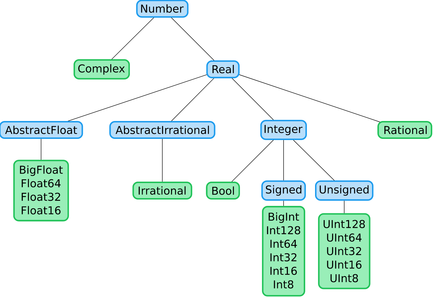
All types depicted in blue are abstract types and the green are concrete types.
Let us consider a type that we have dealt with, for example the Int64 type.
Int64 is a concrete type in Julia, as opposed to an abstract type.
Concretes types are the last in the type hierarchy. In other words, there are no subtypes below Int64 in Julia.
However, there are types that lie "above" Int64 in the type hierarchy.
If you consider the subgraph of Int64 you will see the following.
Int64 <: Signed <: Integer <: Real <: Number <: Any
What this line of code says is that Int64 is a subtype of all the components to the right of it. The <: operator basically says that the left component is a subtype of the right.
In other words, Int64 is a subtype of the Integer type.
The Integer type in this case is a abstract type (which we cover in the section below), since there are subtypes below it (such as Signed and Int64).
You can take a look at the type tree below, which should give some indication on the hierarchy between types. You will see that concrete types are last in the hierarchy (the terminal nodes). Examples include Int128, Int64 and so forth.
print(join(tt(Integer), ""))
Type annotations
We have seen type annotations in our section on functions. In other words, we have something along the lines of x::Int64. This indicates that x is of the type Int64.
This is basically how you tell Julia's compiler that x is of the type Int64.
However, what if we are not sure that x is going to be an Int64, but we know that it will be a number. Then we it is possible to say x::Number.
If we state that something is of a certain type but this is not true, then we will receive a TypeError.
10::Float64
In this error message it tells you: "expected Float64, got a value of type Int64". This means you put down an integer and the compiler was expecting a floating point number. However, if you were uncertain of the type of the input you could have had a more general type, such as Number instead.
10::Number
What can we take from this, in defining functions we can often use type annotations to give an idea fo the type that we expect. There is a good reason for doing this with functions, which is related to the concept of multiple dispatch (a key feature that makes Julia a really special language).
Abstract types
At the core of the type system is the abstract type.
Abstract types cannot be instantiated. This means that we cannot create them explicitly.
They are just a way to organise the types that we have.
If you want to construct an abstract type you would do it as follows.
abstract type Number end # Number is a subtype of Any
abstract type Real <: Number end # Real is a subtype of Number
abstract type AbstractFloat <: Real end # AbstractFloat is a subtype of Real and by extension Number
abstract type AbstractIrrational <: Real end # AbstractIrrational is a subtype of Real and by extension Number
abstract type Integer <: Real end # Integer is a subtype of Real
abstract type Signed <: Integer end # Signed is a subtype of Integer
abstract type Unsigned <: Integer end # Unsigned is a subtype of Integer
Composite types
The things that we can instantiate are called structs.
A struct is a wrapper around some field. These structs are referred to as composite types.
A composite type is a collection of key-value pairs.
This is not easy to understand at first, so let us use some example to make this clear.
In the following example we will be constructing a struct. This struct has no supertype defined here.
struct FirstStruct
    field::Float64
end
This struct contains one field, which is of the type Float64. The input for this struct need to be of type Float64, otherwise the call will not work.
If the type annotation is omitted, Any is used, and such a field may contain any value.
We can create a new instance of the above type by calling FirstStruct as a function.
x = FirstStruct(1.2)
We can access the field value for this composite type via dot notation,
x.field
Happiness example
Next we will combine structs and abstract types.
Remember that abstract types are there to organise the structs.
We start with the highest level type first.
In our example we are going to be creating a Happiness type, which reflects the overall happiness in the economy.
abstract type Happiness end
Next we think about specific subtypes that might be related in some way to happiness within the economy.
In this case I thought about GDP, which contains components such as investment and consumption. These factors might contribute to happiness. GDP is a measure of income, not wealth. So perhaps not the best way to determine happiness, but let us use it.
In addition, health considerations might also be important for happiness within the economy.
You can imagine your own particular type system here.
abstract type GDP <: Happiness end
abstract type Health <: Happiness end
In our example, we can decompose GDP into its to main components. First, we have consumption expenditure on either goods and services. We can think about an increase in consumption indicating higher GDP and therefore greater happiness. This is very superficial, but play along for now.
We can also look at different types of investment. Most important for happiness might be residential investment. However, an increase in investment normally leads to higher job creation and in return higher levels of happiness.
struct Consumption <: GDP
    goods::Float64
    services::Float64
end

struct Investment <: GDP
    inventory::Float64
    residential::Float64
    non_residential::Float64
end
In terms of the health component, let us say that Covid is currently the only disease that people care about. If you have Covid this tends to make you unhappy, and if you don't you are lucky and generally happy about it.
abstract type Sick <: Health end

struct Covid <: Sick
    positive::Bool
end
Now we need to instantiate some of these structs that we have made,
consumption_2021 = Consumption(1205.45, 980.57)
investment_2021 = Investment(130.86, 201.54, 335.12)
covid_pos_2021 = Covid(true)
Now we can create a function that determines if we are happy based on the type of the input. This is where the idea of multiple dispatch comes in.
happy(x::Investment) = true
So far this function, called happy(), gives us the result true if the input type is Investment. Let us extend the function even more.
happy(x::Consumption) = if consumption_2021.goods + consumption_2021.services > 1000 return true end
We now see that the function happy() is a function with two methods. That means that for different inputs it will perform different actions. In this case if the type is Investment the returned value will be true. If the input is Consumption then combined the values of the goods and services fields need to be greater than 1000 for the value to be true.
happy(x::Covid) = false
This last bit of code now tells us that whenever the input type is reflects us being Covid positive, then we are not happy.
map(happy, [consumption_2021, investment_2021, covid_pos_2021])
We can see from the output above that instances of Consumption and Investment return true values. Boolean output of 1 is the same as true. In the case of being Covid positive we are not happy.