Introduction to Machine Learning in Python
- Will take about 1 hour
- Put yourself on mute
- Ask questions in the chat
What is machine learning
Machine learning algorithms build a mathematical model based on sample data, known as "training data", in order to make predictions or decisions without being explicitly programmed to do so. - Wikipedia 2020
We try to create something that learns by itself, given some data, to do things.
How did it all start
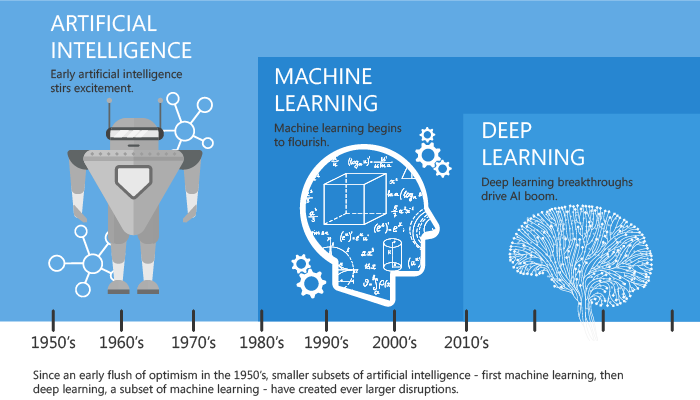
We'll discuss machine learning here. If you are interested in Deep Learning, invite me over another time again :)
How does it compare with programming?
The traditional programming structure

The structure for machine learning

How do we get the right weights (parameters)?

When using in a live system

What are we looking at?
These slides are created with a jupyter notebook, which you'll see as well! Jupyter notebooks are a REPL(Read–eval–print loop)-based interface that is the main tool of data scientists. It allows for rapid experimentation and easy plotting! It is build on IPython, which has a lot of cool things as well!
import numpy as np
??np.arange
import matplotlib.pyplot as plt
x = np.arange(-5, 6)
y = x**2 + np.random.normal(size=(len(x)))
plt.show(plt.scatter(x, y))

import plotly.express as px
px.scatter(y=y, x=x)
Lets start with some data!
We're gonna predict the strain of grape plant that wine was made from!
But first a little bit of software. Python package manager is called pip. It is packaged by default with python. The recommended way of installing python is with Anaconda. Furthermore, we will mainly use these two packages for our work here.
- Scikit Learn - Library that has almost anything you could need for machine learning in python. Install with:
pip install scikit-learn - Pandas- Very widely used library for handling data as tables. You'll see. Install with:
pip install pandas
# Scikit-learn and pandas, two core ML libraries
from sklearn.datasets import load_wine, load_iris
from sklearn.tree import DecisionTreeClassifier
from sklearn import tree
from sklearn.model_selection import train_test_split
import pandas as pd

# Three visualization libraries
import matplotlib.pyplot as plt
import seaborn as sns
import graphviz  # This is a python wrapper around a cli. It requires graphviz in your path.
Now really some data
wine_raw = load_wine(as_frame=True)
wine = wine_raw['frame']
print(wine_raw.target_names)
wine.sample(5)
data/independent variables: All columns except the column we want to predict.
target/dependent variable: The thing we want to predict, so the target column. This value "depends" on the rest of the data.
So lets train a machine learning model!
# Accuracy: how many predictions were correct ->  sum(1=1, 2=2, 3=3)/total
dt = DecisionTreeClassifier(max_depth=2)
dt.fit(wine.drop('target', axis=1), wine.target)
print(f'Accuracy: {dt.score(wine.drop("target", axis=1), wine.target):.02f}')
sample = wine.sample(1)
print(f'Prediction: {dt.predict(sample.drop("target", axis=1)).item()}\nGround truth: {sample["target"].iloc[0]}')
Thanks for coming to my ted talk
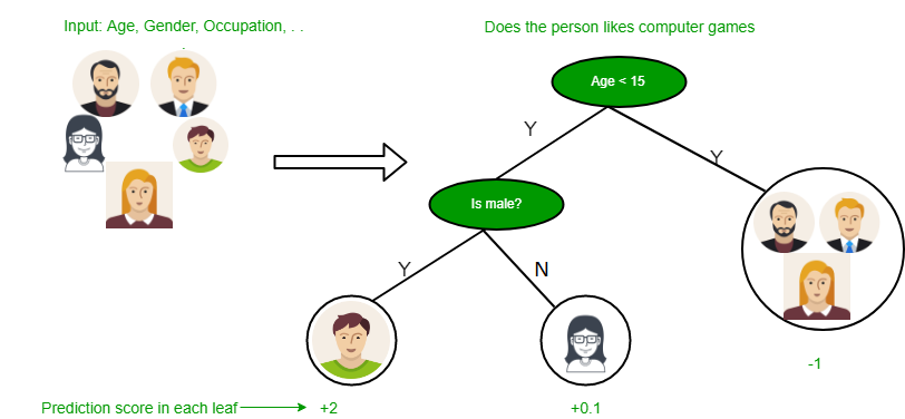
What is a Decision Tree?
Machine learning algorithm that splits on values of certain columns to predict answers. For example, what kind of contacts is someone wearing? Or, what strain of plant was used for a wine?
Why do we like this?
- Doesn't require a lot of feature engineering -> can use the data as is.
- Is very explainable and transparant.
tree_viz
And we can show the importance of each feature
(pd.DataFrame({'importances': dt.feature_importances_}, index=wine.drop('target', axis=1).columns)
     .sort_values('importances', ascending=True)
     .plot(kind='barh')
)

Easy, right?

We might need to do a little due diligence.
How do we know our model is any good?
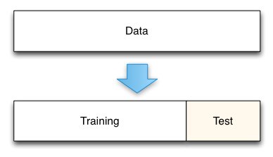
Our model trains on all data and we are also evaluating using that data! That doens't work, the model has already seen that data! So we need a separate data set to evaluate our model.
We split our data into a training set and a test set. The test set is some percentage of the total data set. We will evaluate our model on the test set.

x_train, x_test, y_train, y_test = train_test_split(wine.drop('target', axis=1), wine[['target']], test_size=0.2, shuffle=False)
x_train.shape, y_train.shape, x_test.shape, y_test.shape
x_train.head(2)
y_train.head(2)
dt = DecisionTreeClassifier(max_depth=2, random_state=8)
dt.fit(x_train, y_train)
print(f'Test set accuracy: {dt.score(x_test, y_test):.02f}')
Oh no! Our accuracy dropped! So it performs a bit worse on data it has never seen.
Well, that ok, since it is still pretty high and we were only allowing the model to use two decisions.
What if we allow it to do more?
dt = DecisionTreeClassifier(max_depth=3, random_state=8)
dt.fit(x_train, y_train)
print(f'Test set accuracy: {dt.score(x_test, y_test):.02f}')
dt = DecisionTreeClassifier(max_depth=5, random_state=8)
dt.fit(x_train, y_train)
print(f'Test set accuracy: {dt.score(x_test, y_test):.02f}')
Accuracy goes down!?
dot_data = tree.export_graphviz(dt, out_file=None,
                     feature_names=wine.drop('target', axis=1).columns,
                     class_names=wine_raw.target_names,
                     filled=True, rounded=True,
                     special_characters=True)
tree_viz = graphviz.Source(dot_data)
tree_viz
accuracies = []
max_depths = [1, 2, 3, 5]
for max_depth in max_depths:
    dt = DecisionTreeClassifier(max_depth=max_depth, random_state=8)
    dt.fit(x_train, y_train)
    accuracy = dt.score(x_test, y_test)
    accuracies.append(accuracy)
    print(f'Test set accuracy with max depth of {max_depth}: {accuracy:.02f}')
plt.plot(max_depths, accuracies, 'bo-')
plt.xlabel('Max tree depth')
plt.ylabel('Test set Accuracy')
plt.show()

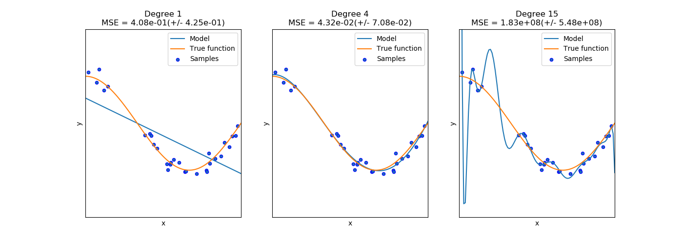
Overfitting
A model or analysis that corresponds too closely or exactly with a particular set of data, and may therefor fail to generalize to new data points. The model is fitting to noise in the train set (not the thing we want to model).
We can try to prevent overfitting by:
- Using more data (not always an option)
- Reduce parameters in the model (Like reducing max depth)
- Regularize the model (Like requiring multiple data points for each leaf-node)
In our case, it means we set the max tree depth to ca. 5, since that seemed to give the best result.
Stepping back a bit
We have seen:
- What a decision tree is
- What a train and test set are
- What overfitting is
To give some extra context:
- This was a supervised machine learning problem
- It was a classification task
Types of machine learning
- Supervised learning - We have labels (Strain of grape plant)
- Unsupervised learning - We don't have labels (We want to find similar data points)
- Reinforcement learning - The algorithms learns from its own predictions (We want to play a game)
Types of supervised learning:
- Classification - Predict one of several classes. (Strain of grape plant, Animal, gender, etc.)
- Regression - Predict a continuous value. (Price, weight, height, etc)
Going a bit deeper: Random Forests
What other machine learning algorithms are there? We have the big brother of decision trees: random forests! They reduce the problem of overfitting of a single decision tree.
- Consist of a large number of individual decision trees (Ensemble)
- Are fit to a random subset of the training dataset (Boosted Aggregation, or bagging)
- Predict with the mode or mean of the predictions from each tree.
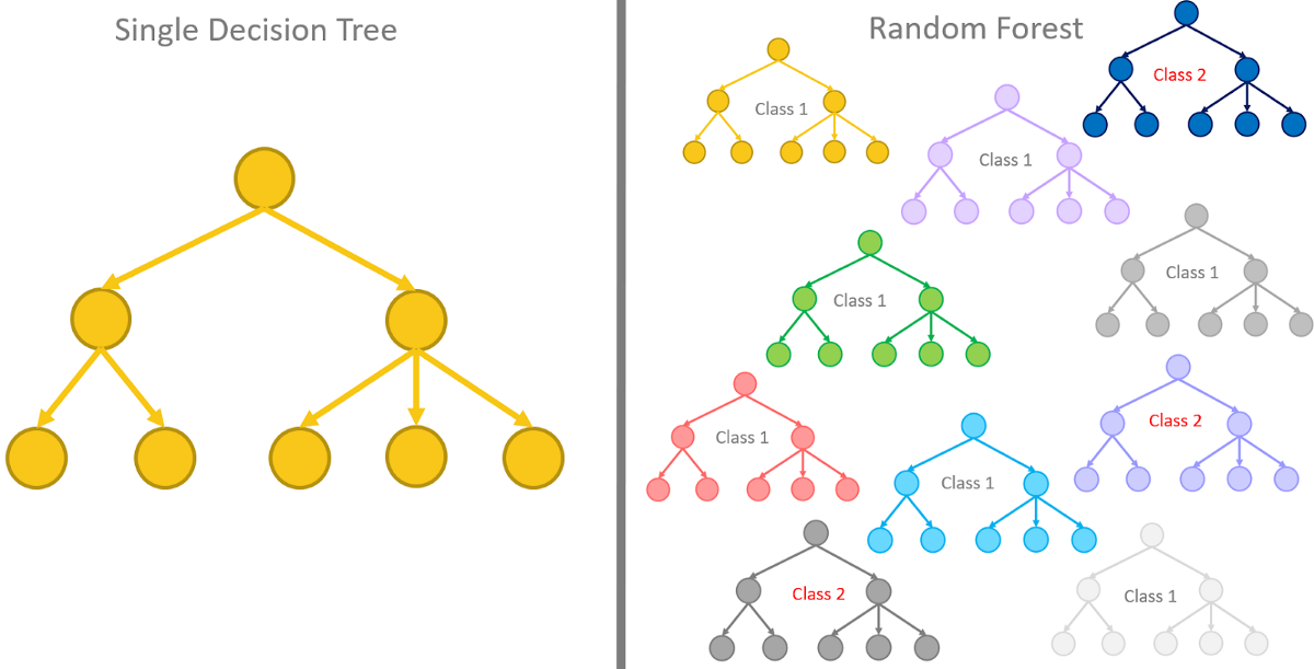
"The low correlation between models is the key. Uncorrelated models can produce ensemble predictions that are more accurate than any of the individual predictions. (...) The reason for this wonderful effect is that the trees protect each other from their individual errors." - Tony Yiu (Understanding Random Forests)
rfs = RandomForestClassifier(n_estimators=5, max_depth=2, random_state=9)
rfs.fit(x_train, y_train)
print('Test set acuraccy of decision tree with max-depth 2: 0.72')
print(f'Test set accuracy: {rfs.score(x_test, y_test):.02f}')
accuracies = []
n_trees = [1, 3, 5, 10]
for n_tree in n_trees:
    rfs = RandomForestClassifier(n_estimators=n_tree, max_depth=3)
    rfs.fit(x_train, y_train.values.reshape(-1))
    accuracy = rfs.score(x_test, y_test)
    accuracies.append(accuracy)
    print(f'Test set accuracy with {n_tree} trees: {accuracy:.04f}')
plt.plot(n_trees, accuracies, 'bo-')
plt.xlabel('Number of Trees')
plt.ylabel('Test set accuracy')
plt.show()

Lets make it a bit more interesting
This was only done on a very simple datasetand we have only looking at the modelling, and nothing else around.
The following example is from a course on ML from the University of San Fransisco. They have a great teacher, Jeremy Howard, who does really well code-first approached to machine learning and deep learning.
- Their lesson on this dataset is at https://github.com/fastai/fastai/blob/master/courses/ml1/lesson1-rf.ipynb.
- Find more of their work on fast.ai
bulldozer_raw = pd.read_csv('train_sample.csv', parse_dates=['saledate'], low_memory=False)[:5000]
display_all(bulldozer_raw[:30])
Bulldozer data
- From a kaggle challenge (https://www.kaggle.com/c/bluebook-for-bulldozers)
- They give you the train data
- They give you validation data without labels.
- They give you test data only in the last week of the challenge.
- They give you the target: predict the sale price of heavy machinery on a certain day
- They give you the metric: The RMSLE (Root mean squared log error) between predicted price and actual price. $$\sqrt{\frac{1}{n}\sum_{i=1}^{n}(\log(y_i+1) - \log( \hat{y}_i+1))^{2}}$$
Now we have:
- Several data types (discrete, continuous, dates, NaNs)
- A continuous target (SalePrice)
- An interesting target, because the error (how wrong we are) is calculated with the log.
The key fields are in train.csv are:
- SalesID: the unique identifier of the sale
- MachineID: the unique identifier of a machine. A machine can be sold multiple times
- saleprice: what the machine sold for at auction (only provided in train.csv)
- saledate: the date of the sale
We need to:
- Preprocess the data
- Feature engineer the data. This means: how to we get suitable features (input for the model) from our data.
We take the log of the prices so we can just calculate the Root Mean Squared Error, which is a very commonly used metric.
The specific log here is the natural logarithm: $$ y' = \log_{e}(y) $$ where $e$ is the mathematical constant $e$)
bulldozer_raw.SalePrice = np.log(bulldozer_raw.SalePrice)
bulldozer_raw.SalePrice
rfs = RandomForestClassifier()
# This will fail due to mixed datatypes
rfs.fit(bulldozer_raw.drop('SalePrice', axis=1), bulldozer_raw.SalePrice)
for col in bulldozer_raw.columns.tolist():
    if bulldozer_raw[col].dtype == 'object':
        bulldozer_raw[col] = bulldozer_raw[col].astype('category')

with pd.option_context('display.max_rows', 100, 'display.max_columns', None):
    print(bulldozer_raw.dtypes)
bulldozer_raw.UsageBand.cat.categories
bulldozer_raw.UsageBand.cat.codes
bulldozer_raw.UsageBand.cat.set_categories(['High', 'Medium', 'Low'], ordered=True, inplace=True)
bulldozer_raw.UsageBand
Dates
Dates contain extremely much information. What kind of information could you get from a date?
- year, month and week
But also
- month begin/end, quarter begin/end, day of week
??add_datepart
add_datepart(bulldozer_raw, 'saledate')
for col in bulldozer_raw.columns:
    if bulldozer_raw[col].dtype.name == 'category':
        bulldozer_raw[col] = bulldozer_raw[col].cat.codes
    if bulldozer_raw[col].dtype ==  'bool':
        bulldozer_raw[col] = bulldozer_raw[col].astype(int)
# This is a regression problem (target is continuous), so we use a regressor instead of a classifier
from sklearn.ensemble import RandomForestRegressor
x_train, x_test, y_train, y_test = train_test_split(bulldozer_raw.drop('SalePrice', axis=1), bulldozer_raw.SalePrice)
rfs = RandomForestRegressor(n_estimators=10)
rfs.fit(x_train.values, y_train.values)
print(f'Test set R2: {rfs.score(x_test, y_test):.04f}')
In statistics, the coefficient of determination, denoted R2 or r2 and pronounced "R squared", is the proportion of the variance in the dependent variable that is predictable from the independent variable(s). https://en.wikipedia.org/wiki/Coefficient_of_determination
preds = np.stack([t.predict(x_test) for t in rfs.estimators_])
preds[:,0], np.mean(preds[:,0]), y_test.iloc[0]
from sklearn import metrics
plt.plot([metrics.r2_score(y_test, np.mean(preds[:i+1], axis=0)) for i in range(10)]);

